Purely electric spin pumping in one-dimension

Abstract

We show theoretically that a simple one dimensional system (such as metallic wire) can display quantum spin pumping possibly without pushing any charge. It is achieved by applying two slowly varying orthogonal gate electric fields on different sections of the wire, thereby generating local spin-orbit (Rashba) terms such that unitary transformations at different places do not commute. This construction is a unique manifestation of a spin-orbit observable effect in purely one dimensional systems with potentials respecting time-reversal symmetry.

A standard way of achieving charge transfer across a conducting system is to apply two gate voltages and change them adiabatically and periodically: Under certain conditions, a charge is transferred across the system during each period. This is referred to as quantum (charge) pumping Thouless ; BPT ; Brouwer ; Avron ; Amnonora1 . In recent years, the concept of pumping with regard to spin polarization has become a focus of attention. One option to get a polarized current is to introduce a Zeeman splitting term prop , or employing ferromagnetic leadsZheng . In some cases it costs a great deal of dissipated energy and besides, time reversal invariance is broken. That motivates the quest for achieving spin pumping without the application of magnetic fields Fazio ; Sharma ; Aono ; Fu (see also Ref.AmnonOra2 where spin filtering is discussed). It is naturally expected that pertinent experiments are rather difficult to carry out, and hence, an obvious desirable property required from a model describing spin pumping is that it should be simple and experimentally feasible.

In the present work we show that spin pumping can be achieved in a simple one dimensional device (wire), by exploiting the spin-orbit (SO) interaction of the electron with electric fields applied on two different sections of the wire (referred below as Rashba barriers). The model is characterized by the following attractive properties: (1) It is purely one dimensional; (2) It enables pure spin (without charge) pumping; (3) The expressions obtained are simple, given in analytic form; (4) It serves as a pedagogical manifestation of the basic concepts of generalized forces and generalized charges; (5) It demonstrates that spin pumping is one of the few manifestations of observable SO effects in purely one-dimensional systems.

Outline. – The order of presentation is as follows: First we derive an expression for the scattering matrix of a single Rashba barrier, and then recall a composition rule for computing the $S$ matrix for scattering off two successive barriers. Once the $S$ matrix of the whole device is obtained, the formalism of Refs. BPT ; Brouwer (see also pmo ) is employed in order to analyze the pumping process. As a by-product an expression for the pumped spin polarization ($\vec{P}$) is derived, that can be regarded as an SU(2) extension of the Brouwer formula for the pumped charge ($Q$), and is somewhat simpler than the one suggested in Ref. Sharma . The conclusion includes a short summary and discussion.

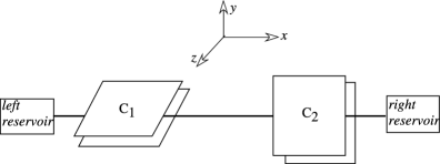
Figure 1: The pumping device (schematic). Electrons move on a one-dimensional wire along the $x$ direction between two reservoirs. Two capacitors $C_{1}$ and $C_{2}$ apply perpendicular electric fields ${\bm{E}_{1}=(0,E_{1},0)}$ and ${\bm{E}_{2}=(0,0,E_{2})}$ whose strength is controlled and varied periodically by an external circuit.

Modeling. – The arena of our discussion is that of non-interacting electrons confined in a straight one-dimensional wire (along $x$) possibly experiencing a scattering potential $V(x)$, and subject to a perpendicular electric field $\bm{E}(x,t)$. The Pauli Hamiltonian is

$$\mathcal{H}=\frac{1}{2\mathsf{m}}p^{2}-\frac{e}{4\mathsf{m}^{2}}(\bm{E}\times\bm{p}-\bm{p}\times\bm{E})\cdot\bm{\sigma}+V(x)$$ (1)

where $\mathsf{m}$ and $e$ are the mass and the charge of the electron, and ${c=\hbar=1}$ units are used. Concretely, we have in mind a simple and experimentally feasible example where the wire passes through a couple of plate capacitors $C_{1}$ and $C_{2}$ with different orientations, as is schematically displayed in Fig. 1. The fields ${\bm{E}_{1}(x)=(0,E_{1},0)}$ and ${\bm{E}_{2}(x)=(0,0,E_{2})}$ are well concentrated at ${x<0}$ and ${x>0}$ segments of the wire and are assumed to be non overlapping.

Since the electric field is perpendicular to the wire, its only effect is to generate an SO interaction of strength $\alpha_{i}(x)={eE_{i}(x)}/{2\mathsf{m}}$ with $i=1,2$ corresponding to the left and right Rashba barriers. The dimensionless parameters that characterize this interaction are

$$\theta_{i}=2\int_{-\infty}^{\infty}\alpha_{i}(x^{\prime})dx^{\prime}\ \ \ \ \ \ \mbox{i=1,2}$$ (2)

The time dependence of $\theta_{1}$ and $\theta_{2}$ is assumed to be periodic and very smooth, justifying the use of the adiabatic approximation. Practically then, the time is used as a parameter that will be employed at a later stage when the spin pumping is discussed (hence it will not be specified before that). Our first goal is to find the $\bm{S}$ matrix for scattering through the system depicted in the above figure. The strategy would be to write down the Pauli equation and solve the scattering problem separately for each barrier thereby obtaining the corresponding $\bm{S}$ matrices $\bm{S}^{(1)}$ and $\bm{S}^{(2)}$ and then combine them to obtain the total $\bm{S}$ matrix.

Scattering from a single Rashba barrier. – The electric field $E_{1}(x)$ in the left barrier is constant deep inside the capacitor and decays as a third power (in distance) outside it. For definiteness let us assume that the capacitor $C_{1}$ is centered at $x=-{L}/{2}$ and that $L$ is sufficiently large so that $E_{1}(x)$ is non-negligible only within ${-L<x<0}$. The Pauli Hamiltonian Eq.(1) for the left barrier can be cast into the following form

$$\mathcal{H}_{1}=\frac{1}{2\mathsf{m}}[p-\alpha_{1}(x)\sigma_{z}]^{2}+v_{1}(x)$$ (3)

where $p$ is the momentum conjugate to $x$. The scalar potential ${v_{1}(x)=V_{1}(x)-\alpha_{1}(x)^{2}/2\mathsf{m}}$ is non-vanishing within the interval ${-L<x<0}$. The later time dependent analysis assumes that it is not changing in time. This assumption is legitimate for realistic circumstances where the $\alpha^{2}$ correction is small Frohlich . Thus, we may start from the stationary Schrödinger equation for scattering at energy $\varepsilon$ through the first barrier, ${\mathcal{H}_{1}\psi_{1}(x)=\varepsilon\psi_{1}(x)}$, where $\psi_{1}(x)$ is a two component spinor.

For the Hamiltonian Eq.(3), the spin projection along the $z$ direction is a ‘good quantum number’. A particle with spin up (an eigenstate of $\sigma_{z}$ with eigenvalue $+1$) experiences a “vector potential” ${A(x)=+\alpha_{1}(x)}$ that can be gauged away, leading to an $A(x)$ independent reflection amplitude $r$, while the transmission amplitude $t$ is multiplied by a phase factor $\mbox{e}^{i\theta_{1}/2}$. A particle with spin “down” would experience a “vector potential” ${A(x)=-\alpha_{1}(x)}$ and therefore would gain upon transmission an opposite phase $\mbox{e}^{-i\theta_{1}/2}$. The scattering of spin “up” and scattering of spin “down” involve different topological phases, turning the effect of SO interaction to be distinct from that of U(1) vector potential. In general the scattered particle may have any spin direction (a superposition of “up” and “down”). Thus, due to SO interaction, different phases are accumulated by the up/down amplitudes of $\psi(x)$, implying that the spin direction is SU(2) rotated, the rotation angle being $\theta_{1}$. From the above analysis it follows that the scattering matrix of the first barrier has the form

$$\bm{S}^{(1)}_{ab}=\left(\begin{matrix}r&0&t\mbox{e}^{-i\theta_{1}/2}&0\cr 0&r&0&t\mbox{e}^{+i\theta_{1}/2}\cr t\mbox{e}^{+i\theta_{1}/2}&0&r&0\cr 0&t\mbox{e}^{-i\theta_{1}/2}&0&r\end{matrix}\right)$$ (4)

where the channel index is ${a=1\uparrow,1\downarrow,2\uparrow,2\downarrow}$. The reflection amplitude $r$ and the transmission amplitude $t$ are determined by the potential $v_{1}(x)$. A more compact way to write this $S$ matrix is,

$$\bm{S}^{(1)}=\begin{pmatrix}R_{1}&T_{1}^{\prime}\\ T_{1}&R_{1}\end{pmatrix}=\begin{pmatrix}r\bm{1}&tU_{1}^{-1}\\ tU_{1}&r\bm{1}\end{pmatrix},$$ (5)

where $\bm{1}$ is the $2\times 2$ identity matrix and $U_{1}$ is an SU(2) rotation matrix defined via Eq.  (4) (see also Eq. (7) below). Within the geometry of Fig. 1, the Hamiltonian for the second system is,

$$\mathcal{H}_{2}=\frac{1}{2\mathsf{m}}[p+\alpha_{2}(x)\sigma_{y}]^{2}+v_{2}(x).$$ (6)

Assuming (just for convenience) that the second barrier has the same reflection and transmission amplitudes ($r$ and $t$), its $S$ matrix has an identical structure as $\bm{S}^{(1)}$ albeit with different spin rotation matrix $U_{2}\neq U_{1}$. Inspecting the kinetic terms of $\mathcal{H}_{1}$ and $\mathcal{H}_{2}$ (see Eqs. (3) and (6)), it is clear that the corresponding spin rotation matrices are,

$$U_{1}=\mbox{e}^{+i\theta_{1}\sigma_{z}/2},\ \ U_{2}=\mbox{e}^{-i\theta_{2}\sigma_{y}/2}.$$ (7)

It is important to notice that $[U_{1},U_{2}]\neq 0$. This non-commutativity of the SU(2) rotations is crucial for the operation of the pumping device, as discussed below.

Scattering from two Rashba barriers. – It is now possible to construct the $\bm{S}=\bm{S}^{(1)}*\bm{S}^{(2)}$ matrix of the whole device by adding the two (non-overlaping) barriers in a series, employing the following prescription comb for calculating the transmission and reflection amplitudes:

$$T=T_{2}(1-R_{1}^{{}^{\prime}}R_{2})^{-1}T_{1},$$

$$T^{\prime}=T_{1}^{{}^{\prime}}(1-R_{2}R_{1}^{{}^{\prime}})^{-1}T_{2}^{{}^{\prime}},$$

$$R=R_{1}+T_{1}^{{}^{\prime}}(1-R_{2}R_{1}^{{}^{\prime}})^{-1}R_{2}T_{1},$$

$$R^{\prime}=R_{2}^{{}^{\prime}}+T_{2}(1-R_{1}^{{}^{\prime}}R_{2})^{-1}R_{1}^{{}^{\prime}}T_{2}^{{}^{\prime}}.$$ (8)

In the absence of SO the transmission and reflection amplitudes due to the total potential $v_{1}(x){+}v_{2}(x)$ are

$$\tau=\frac{t^{2}}{1-r^{2}},\ \ \ \ \rho=r\left(1+\frac{t^{2}}{1-r^{2}}\right).$$ (9)

In the presence of SO, Eqs. (8) imply,

$$\bm{S}=\begin{pmatrix}R&T^{\prime}\\ T&R^{\prime}\end{pmatrix}=\begin{pmatrix}\rho\bm{1}&\tau U_{1}^{-1}U_{2}^{-1}\\ \tau U_{2}U_{1}&\rho\bm{1}\end{pmatrix},$$ (10)

where $U_{1}$ and $U_{2}$ are defined in Eq. (7).

Gauge considerations. – In one dimension, any U(1) gauge potential can be transformed away from the Schrödinger equation. Is it true also for the SO interaction? Let us introduce the transformation

$$\psi(x)=\mbox{EXP}\left[i\int_{-\infty}^{x}\!\!\!\!\!dx^{\prime}\bm{A}(x^{\prime})\right]\Psi(x)\ \equiv\ U(x)\Psi(x)$$ (11)

where $\bm{A}(x)=[\bm{\alpha}\times\bm{\sigma}]_{x}=(0,-\alpha_{2},\alpha_{1})\cdot\bm{\sigma}$. The EXP stands for $x$ ordered exponentiation which is analogous to time ordered exponentiation. The result of the exponentiation is an SU(2) rotation matrix $U(x)$. It is not difficult to verify that $\Psi(x)$ satisfies the time independent equation ${\mathcal{H}_{0}\Psi(x)=\varepsilon\Psi(x)}$ where $\mathcal{H}_{0}$ is obtained from Eq.(3) or Eq.(6) after removing the $\alpha(x)\sigma$ term. Hence, for a general barrier (not necessarily double barrier) the $\bm{S}$ matrix still has the structure as in Eq.(5) / Eq.(10) with the appropriate rotation matrix.

Encouraged by the above observation one may be tempted to conclude that the SO term can be transformed away also in the time dependent pumping formulation. But this is wrong. In the U(1) (charge pumping) formalism the gauge function is ${\Lambda(x)=\int^{x}A(x^{\prime})dx^{\prime}}$ and the time dependence results in an additional term $-d\Lambda/dt$ (electro motive force) that can be absorbed into the definition of the scalar potential $V(x)$. In the SU(2) (spin pumping) scheme the analogous transformation leads to a spin dependent term, and hence the SO nature of the interaction still manifests itself. Therefore in a time dependent pumping problem it is impossible to transform away the SO interaction.

The operation of the pumping device. – We now consider the situation displayed in Fig. 1 where the SO dimensionless parameters $\theta_{1}(t)$ and $\theta_{2}(t)$ of Eq.(2) are controlled by slowly varying the fields inside the capacitors with a common period $2\pi/\omega$. The adiabatic picture implies that the driving frequency $\omega$ is very small compared with other frequency scales of the system. Our goal is to study the pumped charge and the pumped spin polarization during a single period. The generalized conductance is defined as in pmo via the relation:

$$dQ_{a}\ \ =\ \ -\sum_{i=1,2}G^{a,i}(\theta)\ d\theta_{i}$$ (12)

where $dQ_{a}$ is the charge which is pushed into channel $a$ and ${i=1,2}$ specifies the control parameter $\theta_{i}(t)$. If only one control parameter is being manipulated (call it $\theta$), and the practical interest is only (say) in the left lead, then one can use the simpler notations ${dQ_{\uparrow}=-G^{\uparrow}d\theta}$ and ${dQ_{\downarrow}=-G^{\downarrow}d\theta}$. Accordingly the net charge which is pushed into the specified lead is ${dQ=-(G^{\uparrow}+G^{\downarrow})d\theta}$ while the net spin polarization is ${dP_{z}=-(G^{\uparrow}-G^{\downarrow})d\theta}$. In what follows we explain how $dP_{x}$ and $dP_{y}$ can be calculated as well, and show that our pump can generate net spin polarization current while the net charge current is zero at any moment.

Calculation of $G$. – The generalized conductance can be calculated using the Buttiker-Thomas-Pretre formula BPT ; Brouwer . With our notations it reads:

$$G^{a,i}(\theta)\ \ =\ \ \frac{1}{2\pi i}\left[\frac{\partial\bm{S}}{\partial\theta_{i}}\bm{S}^{\dagger}\right]_{aa}\ \ \equiv\ \ -\frac{1}{2\pi}\left[\bm{H}^{(i)}\right]_{aa}$$ (13)

If one regards the $\bm{S}(\theta)$ matrices as a group of unitary transformations, then the $\bm{H}^{(i)}$ are interpreted as their generators. For the problem under consideration:

$$\bm{H}^{(1)}=\frac{1}{2}\begin{pmatrix}|\tau|^{2}\sigma_{z}&\tau\rho^{*}\sigma_{z}U_{1}^{{\dagger}}U_{2}^{{\dagger}}\\ -\tau\rho^{*}U_{2}U_{1}\sigma_{z}&-|\tau|^{2}U_{2}\sigma_{z}U_{2}^{{\dagger}}\end{pmatrix}$$

$$\bm{H}^{(2)}=\frac{1}{2}\begin{pmatrix}-|\tau|^{2}U_{1}^{{\dagger}}\sigma_{y}U_{1}&-\tau\rho^{*}U_{1}^{{\dagger}}U_{2}^{{\dagger}}\sigma_{y}\\ \tau\rho^{*}\sigma_{y}U_{2}U_{1}&|\tau|^{2}\sigma_{y}\end{pmatrix}$$ (14)

Form the above expressions it is manifestly clear that the net charge which is pushed out into (say) the left lead is zero. This is because ${G^{\uparrow}+G^{\downarrow}=0}$ for any of the two leads. But what about the spin polarization current? The latter is determined by ${G^{\uparrow}-G^{\downarrow}}$, and in general it is not zero.

Pumping of spin polarization. – In order to get physical understanding of the spin pumping one should observe that if the channel basis is changed, then $\bm{H}$ undergoes a similarity transformation ${\bm{H}\mapsto\mathcal{T}^{-1}\bm{H}\mathcal{T}}$ where $\mathcal{T}$ is the transformation matrix from the old to the new basis. In particular one is interested in block diagonal $\mathcal{T}$s, such that each of the two $2\times 2$ blocks represents an SU(2) rotation of the axes that are attached to the respective lead. One observes that by an appropriate choice of axes, a given lead-related $2\times 2$ block of a given $\bm{H}$ matrix can be transformed into the canonical form

$$\bm{H}_{\mbox{\tiny lead}}\longmapsto\frac{1}{2}|\tau|^{2}\sigma_{\mbox{\tiny Z}}$$ (15)

where $Z$ is the new $z$ axis. This means that the net spin polarization which is pushed into a lead is

$$dP_{\mbox{\tiny Z}}=|\tau|^{2}\frac{d\theta}{2\pi}$$ (16)

where $\theta$ is either $\theta_{1}$ or $\theta_{2}$. It should be appreciated that the direction ($Z$) of the spin polarization current depends on whether $\theta_{1}$ or $\theta_{2}$ is being changed, and it is not the same for the left and for the right lead. Specifically, if $\theta_{1}$ is being varied, then the spin polarization of the current in the left lead is in the $z$ direction, while in the right lead it is in the $xy$ plane, with an angle $\theta_{1}$ relative to the $y$ direction.

Example. – As an example one can consider the following prototype pumping cycle

$$(\theta_{1},\theta_{2})=(0,0)\mapsto(\pi,0)\mapsto(\pi,\pi)\mapsto(0,\pi)\mapsto...$$ (17)

During the 1st and the 3rd stages of the cycle the spin polarization which is pushed into the left lead is $\pm|\tau|^{2}/2$ in the $z$ direction, while during the 2nd and 4th stages it is $+|\tau|^{2}/2$ in the $y$ direction. Thus we generate per cycle net spin polarization $|\tau|^{2}$ in the $y$ direction, while at any moment the net pumped charge is zero.

SU(2) extension of the Brouwer formula. – For a general pumping cycle the net pumping is given by a line integral over the conductance. Following Brouwer, one can replace this line integral by an area integral using Stokes theorem. Namely,

$$Q_{a}\ \ =\ \ \oint\bm{G}\wedge d\bm{\theta}\ \ =\ \ \iint\bm{C}_{aa}d\theta_{1}d\theta_{2}$$ (18)

where $\bm{\theta}=(\theta_{1},\theta_{2})$, and $\bm{G}=(G^{a,1},G^{a,2})$. In the above expression we have introduced the “rotor” $\bm{C}_{aa}$ of $\bm{G}$. This rotor can be regarded as a diagonal element of the matrix ${\bm{C}=-(1/2\pi)[\partial_{1}\bm{H}_{2}-\partial_{2}\bm{H}_{1}}]$, hence

$$\bm{C}\ =\ \frac{1}{\pi}\Im\left[\left(\frac{\partial\bm{S}}{\partial\theta_{2}}\right)\left(\frac{\partial\bm{S}^{\dagger}}{\partial\theta_{1}}\right)\right]=\frac{1}{2\pi i}[\bm{H}_{2},\bm{H}_{1}]$$ (19)

Note that if one change the channel basis, then $\bm{C}$ undergoes a similarity transformation. Calculating $\bm{C}$ for our model system one observes that the derivatives bring down $\sigma_{y}\sigma_{z}=i\sigma_{x}$ and each $\sigma_{x}$ is rotated by the corresponding SU(2) rotation matrix, by angles $-\theta_{1}$ around $z$ for $U_{1}$ and $\theta_{2}$ around $y$ for $U_{2}$, leading to

$${\bf C}=\frac{i}{4\pi}|\tau|^{2}\begin{pmatrix}U_{1}^{{\dagger}}\sigma_{y}\sigma_{z}U_{1}&0\\ 0&U_{2}\sigma_{y}\sigma_{z}U_{2}^{{\dagger}}\end{pmatrix}$$ (20)

$$=-\frac{1}{4\pi}|\tau|^{2}\begin{pmatrix}\cos\theta_{1}\sigma_{x}+\sin\theta_{1}\sigma_{y}&0\\ 0&\cos\theta_{2}\sigma_{x}-\sin\theta_{2}\sigma_{z}\end{pmatrix}$$

One can re-write the expressions for the pumped charge and the pumped spin polarization in a Brouwer-like style:

$$Q_{\mbox{\tiny lead}}\ \ = \ \ \iint\mbox{trace}(\bm{C}\bm{1}{\mbox{\tiny lead}})d\theta_{1}d\theta_{2}$$ (21)

$$\vec{P}_{\mbox{\tiny lead}}\ \ = \ \ \iint\mbox{trace}(\bm{C}\vec{\bm{\sigma}}{\mbox{\tiny lead}})d\theta_{1}d\theta_{2}$$ (22)

The matrix $\bm{1}{\mbox{\tiny lead}}$ is a projector on (say) the left lead, which means in practical terms that one can keep only the upper right $2\times 2$ block of $\bm{C}$, and sum only over the channels of the left lead. For the model system under consideration we manifestly have zero trace and hence the Brouwer formula gives $Q_{\mbox{\tiny lead}}=0$. This is to be expected when the effect of spin orbit appears as a pure gauge: it affects the wave function merely through an SU(2) phase factor. On the other hand, spin pumping is not zero because ${\bf C}$ is multiplied by spin matrices before being traced, and one can get a non-zero spin polarization $\vec{P}$.

It might be useful to notice that the integral over $\bm{C}$, which is Eq.(22) without the trace, is formally an expression for the spin polarization matrix, rather than for the spin polarization vector:

$$\rho_{\mbox{\tiny lead}}\ \ =\ \ \iint\bm{C}_{\mbox{\tiny lead}}d\theta_{1}d\theta_{2}$$ (23)

Here $\bm{C}_{\mbox{\tiny lead}}$ is the relevant $2\times 2$ block that corresponds to the lead under consideration.

Discussion. – On the practical level it has been demonstrated in this work that it is possible to polarize a neutral spin current using a strictly 1D device with no extra magnetic fields. This should be contrasted with more complicated arrangements that were suggested for this purpose e.g. in Ref.AmnonOra2 . The scheme that has been considered in our analysis is based on a pumping (time dependent) paradigm, instead of the conventional transmission filter paradigm, and at the same time does not involve the use of magnetic fields.

On the mathematical side an extremely simple result for the pumped spin polarization has been obtained, namely Eq.(16). As demonstrated, it can also be formulated as an SU(2) extension of the Brouwer formula for charge pumping, noting that the geometric (Kubo) conductance $G$ is formally a 2-form (curvature), while $C$ is a 3-form (scalar).

We have illuminated the gauge consideration in the theory: while in the time-independent setting it is possible to transform away the SO interaction, in spite of the non-commutativity of the SU(2) gauge transformations, this is no longer true for the time dependent Hamiltonian that describes the pumping scenario.

Acknowledgments. – The research of D.C is partially supported by a grant from the USA-Israel Binational Science Foundation (BSF), and by a grant from the Deutsch-Israelische Projektkooperation (DIP). That of Y.A is partially supported by an ISF grant. N.N. is supported by Grant-in-Aids under Grant No. 19048015, 21244053, and NAREGI Nanoscience Project from the Ministry of Education, Culture, Sports, Science and Technology, Japan.

References

- (1) D. J. Thouless, Phys. Rev. B 27 6083 (1983).
- (2) M. Buttiker, H. Thomas and A Pretre, Z. Phys. B-Condens. Mat., 94, 133 (1994).
- (3) P. W. Brouwer, Phys. Rev. B 58, 10135 (1998).
- (4) J. E. Avron, A. Elgart, G. M. Graf and L. Sadun, Phys. Rev. B 62, 10618 (2000).
- (5) O. Entin-Wohlman and A. Aharony, Phys. Rev. B66, 035329 (2002).
- (6) E.R. Mucciolo1, C. Chamon and C.M. Marcus, Phys. Rev. Lett. 89, 146802 (2002); S.K. Watson, R.M. Potok, C.M. Marcus and V. Umansky, Phys. Rev. Lett. 91, 258301 (2003); C. Bena and L. Balents, Phys. Rev. B70, 245318 (2004); S. M. Watts, C. H. van der Wal and B. J. van Wees, Abstract A22.010, APS March Meeting (2006).
- (7) W. Zheng, J. Wu, B. Wang, J. Wang, Q. Sun and H Guo, Phys. Rev. B68, 113306 (2003).
- (8) M. Governale, F. Taddei and R. Fazio, Phys. Rev. B 68, 155324 (2003).
- (9) P. Sharma and P.W. Brouwer, Phys. Rev. Lett. 91, 166801 (2003).
- (10) T. Aono, Phys. Rev. B 67, 155303 (2003).
- (11) Liang Fu and C. L. Kane, Phys. Rev. B74, 195312 (2006).
- (12) A. Aharony, O. Entin-Wohlman, Y. Tokura and S. Katsumoto, Phys. Rev. B78, 125328 (2008).
- (13) J. Fröhlich and U. M. Studer, Rev. Mod. Phys. 65, 733 (1993).
- (14) D. Cohen, Phys. Rev. B 68, 201303(R) (2003); Phys. Rev. B 68, 155303 (2003).
- (15) See for example: Y. Avishai and J. M.Luck, Phys. Rev. 45, 1074 (1992).