Limitations of model fitting methods for lensing shear estimation

Abstract

Gravitational lensing shear has the potential to be the most powerful tool for constraining the nature of dark energy. However, accurate measurement of galaxy shear is crucial and has been shown to be non-trivial by the Shear TEsting Programme. Here we demonstrate a fundamental limit to the accuracy achievable by model-fitting techniques, if oversimplistic models are used. We show that even if galaxies have elliptical isophotes, model-fitting methods which assume elliptical isophotes can have significant biases if they use the wrong profile. We use noise-free simulations to show that on allowing sufficient flexibility in the profile the biases can be made negligible. This is no longer the case if elliptical isophote models are used to fit galaxies made up of a bulge plus a disk, if these two components have different ellipticities. The limiting accuracy is dependent on the galaxy shape but we find the most significant biases for simple spiral-like galaxies. The implications for a given cosmic shear survey will depend on the actual distribution of galaxy morphologies in the universe, taking into account the survey selection function and the point spread function. However our results suggest that the impact on cosmic shear results from current and near future surveys may be negligible. Meanwhile, these results should encourage the development of existing approaches which are less sensitive to morphology, as well as methods which use priors on galaxy shapes learnt from deep surveys.

1 Introduction

Dark energy dominates the mass-energy of the universe and the goal to discover the nature of dark energy, or even whether it truly exists, is of paramount importance in cosmology. Cosmic shear provides one of the most promising methods for constraining the nature of dark energy (Albrecht et al., 2006; Peacock & Schneider, 2006). Cosmic shear is the mild distortion of distant galaxy images due to the bending of light by intervening matter. Typically galaxy images are stretched by only a few per cent, for example an intrinsically circular galaxy image would become an ellipse with major to minor axis ratio of about 1.06. The clumpier the intervening dark matter, the greater the distortions. Dark energy affects the rate of gravitational collapse, therefore it can be investigated by measuring cosmic shear at different times in the history of the universe.

A number of observational surveys are planned to capitalise on this, including ground-based projects KIlo-Degree Survey (KIDS), Pan-STARRS , the Dark Energy Survey (DES)  and the Large Synoptic Survey Telescope (LSST) , and space missions the International Dark Energy Cosmology Survey (IDECS) or Euclid and/or the Joint Dark Energy Mission (JDEM). If we are to fully utilise the potential of these future cosmology surveys then the potential systematics associated with measuring cosmic lensing must be understood and controlled. The main areas for work are (i) measurement and calibration of galaxy redshifts (ii) measurement and subtraction of galaxy intrinsic alignments and (iii) accurate shear measurement from images. In this paper we focus on the last of these.

Shear measurement is difficult because (i) images are convolved with a kernel due to the atmosphere, telescope optics and measurement devices, (ii) they are then pixelised and (iii) they are noisy mainly due to the finite number of photons collected. The convolution kernel (usually referred to as the point spread function, hereafter PSF) is typically a similar size to the unconvolved galaxy image and is generally not circular. It must be accurately measured either from a detailed model of the telescope or, more usually, from stars in the image, which can be treated as point objects before the convolution. Many works, including this paper, focus on the case where the PSF is perfectly known. However the shear measurement problem is still very difficult due to the high noise levels in the images and the very small signals that need to be measured. The signal-to-noise ratio on shear measurement from any single galaxy image is typically about 0.1, and the signal from many millions of galaxies must be combined to make useful measurements of cosmology.

The Shear TEsting Programme (Heymans et al., 2004; Massey et al., 2007) is a collaborative effort to quantify the biases associated with current shear measurement methods. Crucially, the programme has validated the implementation of the Kaiser et al. (1995) (KSB) method by several groups to obtain shears from real data. In brief, the method measures the quadrupole moments of the image which are combined to estimate the ellipticity of the galaxy. The presence of noise in the images requires the addition of a weighting factor. It is now widely believed however that KSB methods will not be sufficiently accurate to obtain shears from future surveys observing billions of galaxies.

Several groups are working on model-fitting methods to obtain shear, using either Gaussian weighted Hermite polynomials (‘shapelets’) to model the galaxy (Bernstein & Jarvis, 2002; Nakajima & Bernstein, 2007) or elliptical profiles (Kuijken, 1999; Bridle et al., 2002; Irwin et al., 2007; Kuijken, 2006; Miller et al., 2007; Kitching et al., 2008). Alternatively, statistics from shapelets can also be considered as shear estimators that generalise and improve on weighted quadrupole moments (Refregier, 2003; Refregier & Bacon, 2003; Massey & Refregier, 2005). The GRavitational lEnsing Accuracy Testing 2008 (GREAT08) Challenge (Bridle S. et al., 2009) has recently been run to draw expertise from researchers in statistical inference, inverse problems and computational learning.

There is a large variety of galaxy morphologies, whereas the amount of information in any single typical galaxy image is extremely small. Model-fitting methods must therefore make some assumptions. Lewis (2009) has shown that both the PSF and the galaxy shape must be accurately modelled to remove biases; in particular the paper proves that this is a direct result of the symmetries broken by the PSF. In this paper we concentrate solely on the galaxy model, quantifying the bias on the shear for models using elliptical profiles, and assume the PSF is known precisely. In addition we assume infinite signal-to-noise. We first consider the case where the simulated galaxy also has elliptical isophotes, adopting the widely-used de Vaucouleurs and exponential profiles. We also consider more realistic simulated galaxies with non-elliptical isophotes, in particular two-component systems representing early (elliptical) and late-type (spiral or disk-dominated) galaxies in which each component has a different profile shape and ellipticity.

The paper is organised as follows. In Section 2 we summarise the equations governing gravitational shear and describe the method used to quantify the accuracy of the shear measurement method. In addition we discuss the requirements on the accuracy for future dark energy surveys. In Section 3 we describe the simulations used to test the method and in Section 4 we describe the shape measurement method. We then present results for different galaxy shapes in Sections 5 and 6. Finally we discuss the implications of these results on the development of future methods in Section 7.

2 Shear estimation

2.1 Gravitational shear

Light from a source passing a thin lens at position $\mn@boldsymbol{\theta}$ in the lens plane suffers a deflection through an angle $\mn@boldsymbol{\alpha}$ given by

$$\mn@boldsymbol{\alpha}=\nabla\Psi(\mn@boldsymbol{\theta}),$$ (1)

where $\Psi$ is the projected gravitational potential of the lens. If $\mn@boldsymbol{\beta}$ is the true position of the source then the observed position $\mn@boldsymbol{\theta}$ is related to $\mn@boldsymbol{\alpha}$ through the lens equation

$$\mn@boldsymbol{\alpha}(\mn@boldsymbol{\theta})=\mn@boldsymbol{\theta}-\mn@boldsymbol{\beta}.$$ (2)

The gravitational potential of the lens at $\mn@boldsymbol{\theta}$ is related to its surface mass density $\Sigma(\mn@boldsymbol{\theta})$ via the Poisson equation

$$\nabla^{2}\Psi(\mn@boldsymbol{\theta})=\frac{\Sigma(\mn@boldsymbol{\theta})}{\Sigma_{\rm crit}}=2\kappa(\mn@boldsymbol{\theta}),$$ (3)

where $\kappa(\mn@boldsymbol{\theta})$ is the convergence and the critical surface density is

$$\Sigma_{\rm crit}=\frac{c^{2}}{4\pi G}\frac{D_{ls}}{D_{l}D_{s}},$$ (4)

where $D_{s},D_{l}$ and $D_{ls}$ are the angular-diameter distances between the observer and the source, the observer and the lens and between the lens and the source, respectively.

Differentiating Eqns. 1 and  2 with respect to $\mn@boldsymbol{\theta}$ we obtain the Jacobian, or magnification matrix, relating the apparent position $\mn@boldsymbol{\theta}$ to the unlensed position $\mn@boldsymbol{\beta}$ in terms of the gradients of the gravitational potential

$$\emph{{M}}=\frac{\partial\mn@boldsymbol{\beta}}{\partial\mn@boldsymbol{\theta}}=\left(\begin{array}[]{cc}1-\psi_{11}&-\psi_{12}\\ -\psi_{21}&1-\psi_{22}\\ \end{array}\right)$$ (5)

where $\psi_{ij}=\partial^{2}\psi/\partial\theta_{i}\partial\theta_{j}$.

Defining the complex gravitational shear as

$$\gamma=\gamma_{1}+i\gamma_{2},$$ (6)

with

$$\gamma_{1}=\frac{1}{2}\left(\psi_{11}-\psi_{22}\right),\gamma_{2}=\psi_{12}=\psi_{21},$$ (7)

the magnification matrix becomes

$$\emph{{M}}=\left(\begin{array}[]{cc}1-\kappa-\gamma_{1}&-\gamma_{2}\\ -\gamma_{2}&1-\kappa+\gamma_{1}\\ \end{array}\right).$$ (8)

Under this transformation an object with intrinsic complex ellipticity given by

$${e}^{\mathrm{s}}=\frac{a-b}{a+b}e^{2i\phi},$$ (9)

where $a$ and $b$ are the major and minor axes and $\phi$ is the orientation of the major axis from the $x$-axis, is sheared to an object with observed complex ellipticity, $e^{\mathrm{o}}$, given by

$$e^{\mathrm{o}}=\frac{e^{\mathrm{s}}+g}{1+g^{*}e^{\mathrm{s}}}$$ (10)

(Seitz & Schneider, 1997), where $g=\gamma/(1-\kappa)$ is the reduced shear and we have assumed $|g|<1$ (which applies throughout this paper).

2.2 Quantifying the bias on the shear estimator

Shape noise is the statistical noise arising from the random distribution of galaxy shapes. We quantify the bias on the shear measured for different galaxy shapes in the absence of shape noise (i.e. in the limit of an infinite number of galaxy orientations). To achieve this we follow Nakajima & Bernstein (2007) by performing a ‘ring-test’, whereby the same galaxy is rotated around a ring prior to shearing. The mean ellipticity over the ring provides a shear estimate which, as explained below, is free from shape noise to first order. Our shear estimator, $\hat{\gamma}$, is the measured galaxy ellipticity, $e^{\mathrm{m}}$. For a perfect shear measurement method the measured ellipticity is equal to the true observed ellipticity, given in Eq. 10. Even in this case, averaging over galaxy orientations $i$ gives the following expression for the mean true observed ellipticity

$$\langle e^{\mathrm{o}}_{i}\rangle=\gamma^{\mathrm{t}}+\langle e^{\mathrm{s}}_{i}\rangle+\langle(e^{\mathrm{s}}_{i}+\gamma^{\mathrm{t}})(-\gamma^{\mathrm{t}*}e^{\mathrm{s}}_{i}+O(\gamma^{\mathrm{t}*}e^{\mathrm{s}}_{i}))\rangle$$ (11)

where $\gamma^{\mathrm{t}}$ is the true input shear. The term $\langle e^{\mathrm{s}}_{i}\rangle$ is zero for a pair of identical galaxies rotated by 90 degrees from each other. Measuring biases for galaxy pairs was suggested by Nakajima & Bernstein (2007) and adopted in the STEP2 simulations (Massey:2006ha) as a useful method for reducing the intrinsic shape noise. We find that using three linearly spaced pairs of galaxies in the ring-test is enough to reduce the total contribution to the shape noise (i.e. including higher order terms in the sum in Eqn 11) to a negligible level. To test the effects of PSF convolution and pixellisation on the accuracy of our (non-perfect) shear measurement method (i.e. in which $e^{\mathrm{m}}\neq e^{\mathrm{o}}$) we use 18 linearly spaces angles between 0 and 170 degrees. We find that the biases on the shear measured do not change if we double the number of angles used.

We quantify the bias on the shear estimator in terms of multiplicative and additive errors, $m_{i}$ and $c_{i}$ respectively, following Heymans (2006), such that

$$\hat{\gamma}_{i}=(1+m_{i})\gamma^{\rm t}_{i}+c_{i}$$ (12)

where we assume there is no cross contamination of e.g. $\hat{\gamma_{1}}$ depending on the value of $\gamma^{\rm t}_{2}$ or vica versa. We measure $m_{1}$ ($m_{2}$) by shearing along (at 45^∘ to) the $x$-axis with a magnitude of 0.03, i.e. we measure $m_{1}$ by shearing using $\gamma^{\rm t}_{1}=0.03$, $\gamma^{\rm t}_{2}=0$ and $m_{2}$ by shearing using $\gamma^{\rm t}_{1}=0$, $\gamma^{\rm t}_{2}=0.03$.

2.3 Bias requirements for future surveys

Amara & Réfrégier (2008) derived requirements on $m_{i}$ and $c_{i}$ for general current and future surveys covering $A$ deg² of sky, with $n_{\rm gal}$ galaxies per arcmin² and with a median redshift $z_{\rm m}$ (their Eqns. 21 and 22). They consider general functional forms for the redshift evolution of these parameters and require the systematic biases from shear calibration to be less than the random uncertainties, for a two-parameter dark energy equation of state.

We consider 3 sets of survey parameters ($A$, $n_{\rm gal}$, $z_{\rm m}$): (170, 12, 0.8), (5000, 12, 0.8) and ($2\times 10^{4}$, 35, 0.9). These parameter sets are chosen to represent the Canada-France-Hawaii Telescope Legacy Survey (CFHTLS), the Dark Energy Survey (DES) and Euclid. We assume the limit on the additive error $c_{i}$ is equal to the limit on $\sigma_{\rm sys}$ in their Eq. 21 therefore this gives the limits given in Table 1 for each of the three fiducial surveys.

Table 1: Shear measurement requirements on current and future surveys, rounded to one decimal place. For specific survey parameters area $A$, number of galaxies per square arcminute $n_{\rm gal}$ and median redshift $z_{\rm m}$ we show the requirements on the shear multiplicative bias parameters $m_{i}$ and the shear additive bias parameter $c_{i}$. These are combined using the assumptions detailed around Eq. 13 to estimate a required GREAT08 $Q$ value. Survey parameters for upcoming, mid-term and far-future surveys are inspired by the CFHTLS Legacy Survey, the Dark Energy Survey (DES) and Euclid.

Survey	$A$	$n_{\rm gal}$	$z_{\rm m}$	$m_{i}$	$c_{i}$	$Q$
Upcoming	170	12	0.8	0.02	0.001	43
Mid-term	5000	12	0.8	0.004	0.0006	260
Far-future	$2\times 10^{4}$	35	0.9	0.001	0.0003	990

The GRavitational lEnsing Accuracy Testing 2008 (GREAT08) Challenge (Bridle S. et al., 2009) has set a target accuracy level, described by the quality factor, $Q$. The quality factor can be related to the $m$ and $c$ values via the equation

$$Q=\frac{10^{-4}}{\langle m_{i}^{2}\sigma_{\gamma}^{2}+c_{i}^{2}\rangle_{i}},$$ (13)

where $i$ refers to the two shear components and we have written $\sigma_{\gamma}$ as the rms shear used in the simulation (technically this is the reduced shear rather than the shear) and we have assumed that $m_{i}$ and $c_{i}$ are the same for all data. We further assumed that the mean true shear in the simulation is zero. Typically $\sigma_{\gamma}\sim 0.03$ for cosmic shear. The GREAT08 Challenge has set a target accuracy level of $Q=1000$. Therefore, if $m_{i}=0$ then this corresponds to the Euclid requirement on $c_{i}$.

3 Simulations

We next describe the simulations we have used to investigate biases in shear measurement. In Section 5 we investigate shear measurement from simulated de Vaucouleurs and exponential profiles, and in Section 6 two-component galaxies in which each component has a different Sérsic index and ellipticity. Therefore here we discuss the two different galaxy profiles considered, the method used for convolution and the two-component models.

3.1 Galaxy profiles

Galaxies are broadly classified in the literature as ellipticals, pure spheroids or spheroid (bulge) plus disk systems. The de Vaucouleurs profile has long been used to model the light from elliptical galaxies (de Vaucouleurs, 1948) and the exponential profile provides a good description of disk galaxies both in the local universe (Freeman, 1970; Kormendy, 1977; de Jong, 1996; MacArthur et al., 2003) and at high redshift (Elmegreen et al., 2005). Historically, pure spheroids and bulge components have also been modelled using a de Vaucouleurs profile, though recent studies have revealed a range of profile shapes (Graham & Worley, 2008).

Both the de Vaucouleurs and exponential profiles belong to a family of functions known as the Sérsic profiles (Sersic, 1968). The Sérsic intensity at position x is given by

$$I(\emph{{x}})=Ae^{-k[(\emph{{x}}-\emph{{x}}_{0})^{T}\emph{{C}}(\emph{{x}}-\emph{{x}}_{0})]^{\frac{1}{2n}}}$$ (14)

where $\emph{{x}}_{0}$ is the centre, $A$ is the peak intensity, $n$ is the Sérsic index and C (proportional to the inverse covariance matrix if $n=0.5$) has elements

$$C_{11}=\left(\frac{\rm cos^{2}\phi}{a^{2}}+\frac{\rm sin^{2}\phi}{b^{2}}\right)$$ (15)

$$C_{12}=\frac{1}{2}\left(\frac{1}{a^{2}}-\frac{1}{b^{2}}\right)\rm{sin}(2\phi)$$ (16)

$$C_{22}=\left(\frac{\rm sin^{2}\phi}{a^{2}}+\frac{\rm cos^{2}\phi}{b^{2}}\right)$$ (17)

where $\phi$ is the angle (measured anti-clockwise) between the $x$-axis and the major axis of the ellipse and the minor to major axis ratio is $b/a$. The Sérsic index defines the profile ‘type’, with $n=0.5,1$ and $4$ for Gaussian, exponential and de Vaucouleurs profiles respectively. If $k$ is defined as $k=1.9992n-0.3271$ then for a circular profile $r_{\rm e}=a=b$, referred to as the ‘effective radius’ or ‘half-light radius’, is the radius enclosing half the total flux. (Note that for a Gaussian profile $a^{2}$ and $b^{2}$ are the 2D variances if $k=0.5$; for the exponential profile $h=a=b$ is known as the ‘scale length’ when $k=1$.) The full width at half-maximum intensity (FWHM) is related to the effective radius (for a circular profile) via

$$\mathrm{FWHM}=2r_{\mathrm{e}}\left(\frac{\ln 2}{k}\right)^{n}.$$ (18)

Thus for similar effective radii the FWHM of galaxies modelled by Sérsic indices ranging between 0.5 and 4 vary by nearly 4 orders of magnitude. The total flux (integrated to infinity) emitted by a galaxy described by a Sérsic profile with index $n$ is given by

$$F=2\pi nk^{-2n}r_{\rm e}^{2}\Gamma(2n)I_{0}$$ (19)

where $\Gamma$ is the gamma function.

3.2 Shear and Convolution

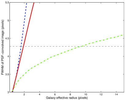
Figure 1: Relationship between the FWHM of the PSF-convolved image and the effective radius of the galaxy. Curves are shown for Gaussian (blue dashed), exponential (red solid) and de Vaucouleurs (green dash-dot) profiles. The horizontal curve (black dashed) shows the FWHM of the PSF-convolved galaxy image used in this paper.

We model the PSF as a single Gaussian aligned along the $x$-axis with ellipticity $e_{\rm p}=0.05$ and FWHM of 2.85 pixels. We define the FWHM of an elliptical object such that the area of the ellipse is equal to the area of a circle with the same FWHM. The default value used for the galaxy ellipticity is $e=0.2$. The galaxy size is chosen such that the FWHM of the PSF-convolved image is 1.5 times that of the PSF . Galaxies smaller than this are generally cut from catalogues used in weak lensing analyses.

We use Eqn. 10 to calculate the ellipticity and orientation of the sheared galaxy at each point in the ring. The major axis of the ellipse is held constant at the pre-lensed value and the minor axis adjusted to obtain the correct, post-shear ellipticity. For bulge plus disk galaxies we shear each component separately.

Fig 1 shows the relationship between the galaxy effective radius and the FWHM of the PSF-convolved image for Gaussian, de Vaucouleurs and exponential profiles. The horizontal dashed line shows the value used in this study. Fig. 4 shows cross-sections through the galaxy and PSF-convolved galaxy profiles for the chosen galaxy parameters, compared with a Gaussian galaxy image. We see that the de Vaucouleurs has an extremely sharp galaxy profile before the PSF convolution, and larger wings after convolution.

By default the galaxy is convolved numerically with the PSF on a large, fine grid $(25\times 45)^{2}$ pixels in size. The PSF FWHM is sampled by $(2.85\times 45)$ pixels. Following the convolution the grid is binned up by a factor of 45 to obtain a square image 25 pixels across in which the FWHM of the PSF is 2.85 pixels. Finally, we cut the grid down to obtain a postage stamp 15 pixels across. We try increasing the resolution used for the convolution such that the PSF FWHM is sampled by $(2.85\times 55)$ pixels. The grid is $(25\times 55)^{2}$ pixels in size and, following the convolution, is binned up by a factor of 55. We also try increasing the size of the grid used for the convolution to $(31\times 45)^{2}$ pixels, keeping the PSF FWHM at the default value and binning up by a factor of 45. In both cases it is the central $15^{2}$ pixels which are analysed. We find that the results do not change when we increase either the resolution or the grid size used for the convolution.

The true galaxy centroid is at the centre of the postage stamp. We find the results are largely insensitive to changes in the centroid position within the central pixel.

3.3 Two-component models

As discussed above, the de Vaucouleurs and exponential profiles are widely used to describe the light distribution in elliptical and disk galaxies. However, real galaxies do not have constant ellipticity isophotes. Therefore in this paper we also explore galaxies with both a bulge and a disk component and, crucially, with non-constant ellipticity isophotes, since we allow the bulge and disk to have different ellipticities.

We consider two different two-component systems: one which closely models realistic spiral (disk-dominated) galaxies, and one which represents ellipticals with a small disk (exponential) component. For the spiral galaxies the bulge is modelled as a Sérsic profile with index 1.5. While for many years it was believed that bulges were universally described by the $r^{1/4}$ model (de Vaucouleurs, 1948, 1958; de Vaucouleurs & Pence, 1978), it is now generally accepted that most bulges have Sérsic indices $n<4$ (Graham, 2001; MacArthur et al., 2003; Balcells et al., 2003; Laurikainen et al., 2006; Graham & Worley, 2008) and typically between $\sim 1-2$ for a range of Hubble types (Graham & Worley, 2008, see their figure 3). Studies also suggest that the bulge-to-disk size ratio is reasonably independent of Hubble type, with Graham & Worley (2008) finding a median value for $r_{e}/h$ equal to 0.22. We adopt a similar size ratio, with $r_{\rm d}/r_{\rm b}$ equal to 7.5, where $r_{\rm d}$ and $r_{\rm b}$ are the disk and bulge effective radii, respectively. Our second model is chosen to represent ellipticals, which are well-described by de Vaucouleurs profiles. We add a small exponential component such that $r_{\rm d}/r_{\rm b}$=0.5. For both models the bulge and disk ellipticities are set equal to $e_{\rm b}=0.05$ and $e_{\rm d}=0.2$ respectively. The bias on the shear is measured for a range of bulge-to-total ($B/T$) flux ratios between 0 and 1. At each $B/T$ value the ratio $r_{\rm d}/r_{\rm b}$ is held constant and the bulge and disk effective radii computed for circular PSF and galaxy profiles such that the FWHM of the PSF-convolved image is 1.5 times the FWHM of the PSF. The total flux in each galaxy component is calculated by integrating the flux from $r=0$ to infinity, as given in Eqn. 19. The bulge and disk effective radii are then adjusted to keep the area of each component constant as the ellipticity is increased from zero.

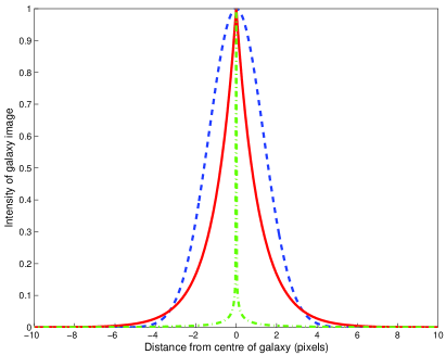
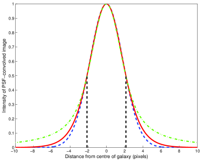
Figure 2: Cross-sections through the centre of a Gaussian (blue dashed), exponential (red solid) and de Vaucouleurs (green dash-dot) galaxy (top) and PSF-convolved galaxy (bottom). The PSF is a Gaussian with FWHM equal to 2.85 pixels. The FWHM of the PSF-convolved image (shown by the vertical black dashed lines) is 1.5 times the FWHM of the PSF.

4 Model fitting using sums of Gaussians

In this paper we model galaxies as a sum of co-elliptical (homeoidal) Gaussians of varying size and amplitude. This model was first suggested by Kuijken (1999), and developed by Bridle et al. (2002) into a publicly available code (im2shape) which has been used to measure cluster masses (e.g. Cypriano et al., 2004) and tested in the STEP1 simulations (Heymans, 2006). We stress that the results found in this paper are general for all models adopting elliptical isophotes since any such model can be completely described in terms of a sum of Gaussians. Adopting a sum of Gaussians to model the galaxy has the particular advantage that the convolution with the PSF can be carried out analytically (assuming the PSF is also modelled as a sum of Gaussians).

If the PSF and galaxy intensity profiles are of the form

$$I_{\rm p}(\emph{{x}})=\frac{k}{\pi}|\emph{{C}}_{\rm p}|^{\frac{1}{2}}e^{-k(\emph{{x}}-\emph{{x}}_{0})^{T}\emph{{C}}_{\rm p}(\emph{{x}}-\emph{{x}}_{0})}$$ (20)

and

$$I_{\rm g}(\emph{{x}})=A_{\rm g}e^{-k(\emph{{x}}-\emph{{x}}_{0})^{T}\emph{{C}}_{\rm g}(\emph{{x}}-\emph{{x}}_{0})}$$ (21)

respectively, then the PSF-convolved intensity for a sum of $n_{\rm g}$ Gaussians is given by

$$I_{\rm gp}(\emph{{x}})=\sum_{i=1}^{n_{\rm g}}A_{\rm g,\it i}\frac{|\emph{ {C}}_{\rm gp,\it i}|^{\frac{1}{2}}}{|\emph{{C}}_{\rm g,\it i}|^{\frac{1}{2}}}e^{-k(\emph{{x}}-\emph{{x}}_{0})^{T}\emph{{C}}_{\rm gp,\it i}(\emph{{x}}-\emph{{x}}_{0})}$$ (22)

where

$$\emph{{C}}_{\rm gp,\it i}=\frac{1}{|\emph{{C}}_{\rm p}+\emph{{C}}_{\rm g,\it i}|}(|\emph{{C}}_{\rm p}|\emph{{C}}_{\rm g,\it i}+|\emph{{C}}_{\rm g,\it i}|\emph{{C}}_{\rm p}).$$ (23)

The centre, ellipticity and orientation of each Gaussian used to model the galaxy are tied. Thus the number of free parameters in the fit is 4 ($\emph{{x}}_{0},e,\phi$) plus $2n_{\rm g}$ ($n_{\rm g}A_{i},n_{\rm g}a_{i}$). The best-fit parameters are found using $\chi^{2}$-minimisation. We speed up the calculation by computing the normalisations of the Gaussians analytically. This is possible because the model is linear in these parameters.

Images are generated on a grid $15^{2}$ pixels in size. The intensity in each pixel is the sum of the intensity computed at the centres of $n_{\rm p}^{2}$ sub-pixels, where we refer to $n_{\rm p}$ as the pixel integration level. The default pixel integration level used in the simulated galaxies is $n_{\rm p}$=45 (see Section 3.2).

5 Results for galaxies with elliptical isophotes

In this Section we simulate galaxies with elliptical isophotes and fit them with different elliptical isophote models. First we try using a single Gaussian when fitting an exponential or de Vaucouleurs profile. We explain our results qualitatively using a one-dimensional toy model. Then we use multiple Gaussians to allow a more accurate fit to the simulations.

5.1 Using the wrong elliptical isophote model

We first ask whether model fitting using a single Gaussian provides an unbiased shear estimate for a galaxy with elliptical isophotes. We use two different profiles to simulate the true galaxy shape: a de Vaucouleurs and an exponential. The default model for the PSF is a single Gaussian aligned along the $x$-axis with perfectly known ellipticity and size. We first investigate how shear measurement biases vary with the size of the pixels used for the observation when the wrong elliptical isophote model is used. We calculate the biases both with the default PSF model and with the PSF set to a delta function. The default value used in this paper for the PSF FWHM is 2.85 pixels, but in Fig 3 we vary the resolution from 1 to 15 pixels per PSF FWHM, while keeping the relative size of the galaxy and PSF the same. For the case where the PSF is a delta function the galaxy size is set equal to that computed for the default PSF model (thus the galaxy size is the same at each point on the $x$-axis in Fig 3).

We ensure that the resolution is the only quantity which changes as the PSF FWHM is increased. This is achieved by convolving the galaxy with the PSF on a large, fine grid and then binning the pixels to obtain images with decreasing resolution. The convolution is carried out as described in Section 3.2, on a grid $(25\times 45)^{2}$ pixels in size, except here the PSF FWHM is sampled by 45 pixels instead of ($2.85\times 45$) pixels. The grid is then binned by a factor of 3 (5,9,15,45) to obtain an image in which the PSF FWHM is 15 (9,5,3,1) pixels. The pixel integration level used in each pixel in the galaxy and PSF images prior to the convolution is 1, thus each binned PSF-convolved image has a pixel integration level equal to the binning factor. At each PSF resolution we use the same pixel integration level in the galaxy model as used in the simulated galaxy image.

The dashed lines in Fig 3 show the results for a delta function PSF. The shaded regions show the requirements on $m_{i}$ and $c_{i}$ given in Table 1. The upper edge of each shaded region (from bottom to top) shows the upper limit on the bias allowed for far-future, mid-term and upcoming surveys respectively. The additive shear calibration biases $c_{1}$ and $c_{2}$ are always zero when no PSF is used. This is not surprising since there is no preferred direction in which the shear could be biased, since the galaxy direction has been averaged out in the ring-test. The pixels do impose a preferred orientation to the image, but any biases would be the same along the $x$ and $y$ axes and thus positive and negative biases to $c_{1}$ and $c_{2}$ are expected to cancel. We see $m_{1}$ and $m_{2}$ decrease as the resolution increases, falling well below forseeable observational requirements (upper edge of grey band). We discuss the cause of the bias for low resolution images below. These results indicate that in the limit of infinitely small pixels, model-fitting using a single Gaussian provides an unbiased estimate of the shear of any two-dimensional profile with constant ellipticity isophotes. This agrees with the more general result found by Lewis (2009) that, for the case where there is no PSF, any (wrong) galaxy model will provide unbiased results.

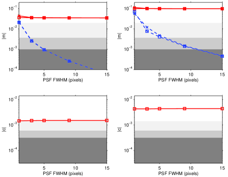
Figure 3: Multiplicative (top) and additive (bottom) biases for exponential (left) and de Vaucouleurs (right) profiles as a function of the number of pixels inside the FWHM of the PSF both with (red solid) and without (blue dashed) the PSF included. Open squares (crosses) show $m_{1}$,$c_{1}$ ($m_{2}$,$c_{2}$). Any values of $m_{i}$ and $c_{i}$ not seen in the plot lie below the minimum value on the $y$-axis. The upper edge of each shaded region (from bottom to top) shows the upper limit on the bias requirements for general far-future, mid-term and upcoming surveys respectively. The survey parameters are given in Table 1. The lower limit on the $y$-axis is an order of magnitude less than the requirements for the far-future survey. The top unshaded region is shown for clarity.

The solid lines in Fig. 3 show the results when the PSF is included. The biases are now significant, independent of the pixel size. In particular, $c_{1}$ is significant, even though the PSF model is known precisely. This is because in general the angle between the PSF and the galaxy is different for each galaxy in a pair in which the $e_{1}$ components cancel. The ring-test may be constructed so that $c_{2}$ is close to zero. This provides a useful check on our method. This is simply achieved by aligning the PSF along the $x$-axis and including the mirror image of each galaxy pair in the $y$-axis. This ensures that the $e_{2}$ components cancel for image pairs in which the angle between the PSF and the galaxy is the same (except for the galaxy pair at 0 and 90 degrees).

The biases for the de Vaucouleurs profile (right hand panel) are larger than for the exponential profile, which is not surprising considering that it is even further from the single Gaussian used in the fit. Inserting the bias values into Eq. 13 for the exponential galaxy simulation (left-hand panel) gives $Q\sim 30$, and for the de Vaucouleurs galaxy gives $Q\sim 6$.

5.2 A qualitative explanation

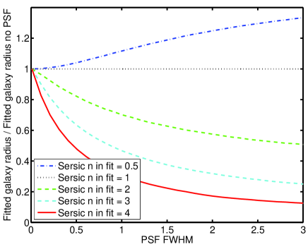
Figure 4: Fitted galaxy size as a function of PSF size for a range of fitted profiles (Sersic index = [ 0.5 1 2 3 4] from top to bottom). A one-dimensional exponential galaxy was simulated, convolved with a known Gaussian PSF and fitted with a one-dimensional Sersic profile. The y axis shows the fitted galaxy size divided by the fitted galaxy size in the absence of a PSF (PSF FWHM = 0).

We explain this result qualitatively using Fig 4, which shows results from a toy problem using a one-dimensional image of infinite resolution. We simulate a galaxy with a one-dimensional exponential profile and convolve it with a Gaussian PSF. The convolved image is then fitted with a Sersic profile convolved with the correct PSF. The galaxy size (scale radius) is varied to find the best-fit, and this is compared to the best-fit in the absence of a PSF. The best-fit size of the galaxy is either over-estimated or underestimated, depending on the value of the Sersic index. The amount by which it is over- or under-estimated increases as the PSF size increases relative to the galaxy. Fitting a Gaussian galaxy profile (Sersic index = 0.5) causes the fitted galaxy radius to be more overestimated the larger the PSF is, relative to the galaxy size.

Consider now a two-dimensional image of a galaxy with elliptical isophotes aligned along the $x$-axis. Very roughly we can consider biases in the measured ellipticity by considering a one-dimensional slice along the $x$-axis, where the galaxy radius is at its largest relative to the PSF, and then a one-dimensional slice along the $y$-axis where the galaxy radius is at its smallest. For an elliptical galaxy, therefore, we expect that if we use a Gaussian to model the galaxy the size of the major axis will be over-estimated less than the minor axis. This will result in a more circular best fit object, and the shear will be biased low. By contrast, if instead we fit the exponential galaxy using a de Vaucouleurs profile then, using similar arguments, the estimated shear will be biased high.

This conclusion can also be seen qualitatively by considering the two-dimensional image that is being fit. Without the PSF, each point around an elliptical isophote has equal weight in the $\chi^{2}$, but when the PSF is added, different parts of the galaxy profile are weighted differently.

In summary, the presence of a convolution causes a bias in the measured shear of an elliptical object, if the wrong profile is assumed.

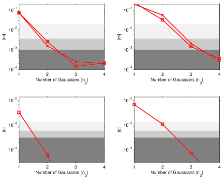
Figure 5: Multiplicative (top) and additive (bottom)biases for exponential (left) and de Vaucouleurs (right) profiles as a function of the number of Gaussians used in the fit. The PSF is included. The pixel integration level $n_{\rm p}$ is 13. Open squares (crosses) show $m_{1}$,$c_{1}$ ($m_{2}$,$c_{2}$). The $c_{2}$ values are smaller than the minimum on the $y$-axis. Shaded regions as in Figure 3.

5.3 Allowing the right elliptical isophote model

We have found that to obtain an unbiased estimate of the galaxy ellipticity, even when the PSF is known and the pixels are small, the galaxy must be modelled well. Next we improve our model by increasing the number of Gaussians used in the sum. An infinite number of homeoidal Gaussians would allow perfect reconstruction of any elliptical isophote galaxy. In Fig 5 we show the biases as a function of the number of Gaussians used. We see that the biases reduce to below far-future requirements for both galaxy profiles when 4 Gaussians are used. For galaxies with an exponential profile only 3 Gaussians are required in the sum. Note that we do not tune practical computational parameters (especially number of sub-pixels used for pixel integration) for points which already lie well below the requirements for future surveys (darkest shaded area).

In Fig 6 we plot the biases as a function of the number of sub-pixels used in the pixel integration. The $x$-axis shows the number of sub-pixels $n_{\rm p}$ in one direction, so the pixel integration sums over values in $n_{\rm p}^{2}$ sub-pixels. Recall that the default value used e.g. in Fig 5 was $n_{\rm p}=13$. Specifically, the biases flatten when limited by the number of Gaussians, and decrease when limited by the pixel integration level. If a small number of sub-pixels are used in the fit then the galaxy is more elliptical than in the unpixellated case. This results in an estimated ellipticity which is rounder than the true ellipticity. This effect however cancels out in the ring-test and the decrease in bias with increasing pixel integration is entirely a result of the improvement in the pixel model. We see that $n_{\rm p}\sim 10$ is more than sufficient for forseeable future surveys, and $n_{\rm p}\sim 5$ is sufficient for mid-term surveys. However $n_{\rm p}\sim 1$ is insufficient even for current surveys.

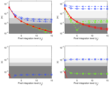
Figure 6: Multiplicative (top) and additive (bottom) biases for exponential (left) and de Vaucouleurs (right) profiles as a function of the pixel integration level, $n_{\rm p}$. Blue dot-dash, green dashed and red solid curves show the biases when 2, 3 and 4 Gaussians are included in the model respectively. Results for 1 Gaussian are larger than the maximum value on the $y$-axis. The PSF is included. Squares (crosses) show $m_{1}$,$c_{1}$ ($m_{2}$,$c_{2}$). Shaded regions as in Figure 3.

6 Results for bulge plus disk galaxies

So far all our simulated galaxies have had elliptical isophotes. However this is not the case in the universe, and the simple deviation we consider in this paper is a two-component bulge plus disk model. In Section 3.3 we described two fiducial two-component models, one to model a spiral galaxy with a bulge, and one to model an elliptical galaxy with a small disk. We repeat the previous shear measurement bias analysis, always using an elliptical isophote model in the fit, despite the non-elliptical isophotes of the simulated images. The purpose is to see whether elliptical isophote models can be used for shear measurement from non-elliptical isophote galaxies.

In Fig. 7 we plot the biases for both two-component models as a function of the number of (co-elliptical) Gaussians used in the fit. For reference, we also show the results when the bulge ellipticity is equal to the disk ellipticity ($e_{\rm b}=e_{\rm d}=0.2$), i.e. the simulated galaxy has elliptical isophotes. When the bulge and disk ellipticity are the same the biases decrease as the number of Gaussians used in the fit increases. This type of behaviour was already seen in Fig. 5, and the results are slightly different now due to the different galaxy profile arising from the sum of exponential and de Vaucouleurs components.

When the bulge and disk have different ellipticities, however, the bias is not reduced by increasing the number of Gaussians beyond $n_{\rm g}=3$. We have checked that this bias is not due to the finite resolution used for the pixel integration. We conclude that it is the failure of the model to take account of galaxies with varying ellipticity isophotes.

We next investigate how the size of the bias depends on the amount of flux in each component. In Fig 8 we plot the biases as a function of the bulge-to-total flux ratio for the spiral and elliptical galaxy models for $n_{\rm g}=4$. Again, we include a reference curve for the case where the bulge and disk ellipticity are equal. As expected, the biases fall to the residual level as $B/T$ approaches zero or unity. The biases differ from the reference curve for $B/T=1$ because the bulge ellipticity is 0.05 for the solid curve but 0.2 for the dashed (reference) curve. The elliptical-like galaxy (left panel) has negligible additive biases, and has multiplicative biases below the requirements of upcoming mid-term surveys at all bulge-to-total ratios. The behaviour at $B/T=0.7$ is due to a change in sign of $m_{i}$ from negative at lower $B/T$ values to positive at higher $B/T$ values.

For the spiral galaxy model both additive and multiplicative biases peak at $B/T\sim 0.2$. The multiplicative bias at this $B/T$ is worse even than the requirements for upcoming surveys. The additive bias is slightly above the requirements for far-future surveys. Most disk galaxies have $B/T<1/3$ (Kormendy, 2008), with a median value of 0.24 for early-type spiral galaxies (Sa-Sb) and 0.04 for late-type spiral galaxies (Scd-Sm) (Graham & Worley, 2008). It is likely that on averaging over all galaxy types the biases are lower than the requirements for upcoming surveys. However, the exact bias for any particular survey will need to be calculated incorporating the galaxy selection criteria and point spread function.

7 Discussion

To fully capitalise on the potential of gravitational lensing as a cosmological probe biases on galaxy shear estimates must be reduced to the sub-percent level. In this paper we have shown that the effects of convolution with the PSF makes this a non-trivial problem. In particular, the unlensed galaxy must be very accurately modelled even if the PSF is known precisely and the pixels are small. We have isolated this effect by restricting our investigation to noise-free images.

We have illustrated that fitting a single elliptical Gaussian to an elliptical exponential or de Vaucouleurs profile causes no bias on the measured shear, in the unrealistic case where the pixels are infinitely small and there is no PSF. For the fiducial galaxy size we chose, application of a realistic PSF causes a significant shear measurement bias, too large even to use single-Gaussian fitting for current cosmic shear data. This illustrates the general point that even if galaxies have elliptical isophotes, a model-fitting method must use a realistic galaxy profile. We explained this qualitatively by considering a one-dimensional toy model.

Lewis (2009) proved that the presence of a PSF will result in biased shear estimates when the wrong galaxy model is used. In this paper we have quantified the level of the bias when the wrong model used is a sum of co-elliptical Gaussians, but stress that our results are general for any model-fitting method using elliptical profiles. We find that if galaxies have elliptical isophotes then a sum of 4 Gaussians is sufficient for future surveys. For bulge plus disk galaxies increasing the number of Gaussians in the model beyond $\sim 3$ does not significantly reduce the biases.

Earlier versions of LensFit (Miller et al., 2007; Kitching et al., 2008) used a de Vaucouleurs profile to fit galaxies of all types, including exponentials. Thus this is expected to lead to a small residual bias. We found that using an overly flat profile (Gaussian) the shears were biased low relative to the truth. Our toy model predicts that fitting an overly peaky profile (e.g. a de Vaucouleurs to an exponential) will overestimate the shears.

Im2shape (Bridle et al., 2002) fits a sum of co-elliptical Gaussians, however there is usually no strong prior on the relative sizes and amplitudes of the components. Therefore when applied to noisy data it is possible that they might not sum to make a particularly peaky profile, and may produce results closer to those expected from fitting a single Gaussian. This could be rectified by applying priors to the relative sizes and amplitudes of the Gaussians, however for best results these priors should be tuned to the expected profiles in the data.

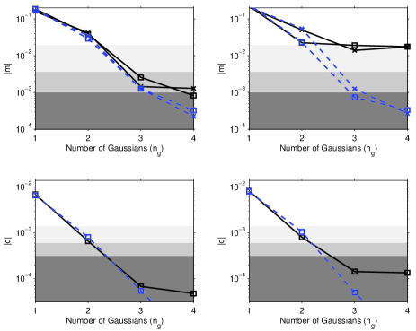
Figure 7: Multiplicative (top) and additive (bottom) biases for two-component galaxies with $r_{\rm d}/r_{\rm b}$ equal to 0.5 (left) and 7.5 (right) as a function of the number of Gaussians used in the fit. The Sérsic index of the bulge is 4 (left) and 1.5 (right) and in both cases the disk is an exponential. Blue dashed and black solid lines show results for the case where the bulge and the disk have the same ellipticity ($e_{\rm b}=e_{\rm d}=0.2$) and different ellipticities ($e_{\rm b}=0.05$, $e_{\rm d}=0.2$) respectively. The bulge to total flux ratio is 0.8 (left) and 0.3 (right). Shaded regions as in Figure 3.

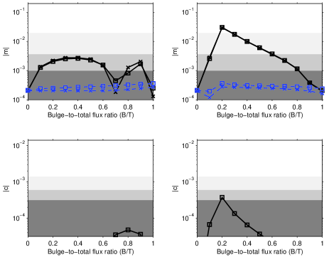
Figure 8: Multiplicative (top) and additive (bottom) biases for elliptical (left) and spiral (right) two-component galaxies as a function of the bulge-to-total flux ratio. Black solid and blue dashed curves as in figure 7. Shaded regions as in Figure 3.

This result may also be relevant for shapelets methods, which are based on a Gaussian. If only a low order shapelet expansion is used then the profile will be less centrally peaked, and have smaller wings, than an exponential or de Vaucouleurs. A similar expansion based on the sech function has been proposed to address these problems (van Uitert & Kuijken in prep).

Model-fitting techniques adopting co-elliptical profiles (Bridle et al., 2002; Kuijken, 2006; Miller et al., 2007; Kitching et al., 2008) cannot, by definition, provide an exact fit to multi-component galaxies with varying ellipticity isophotes. We find that this introduces a fundamental limit to the accuracy of these methods which can produce biases on shear measurements from individual galaxies which are too large for future surveys. The size of the bias depends on the true galaxy morphology, and we investigate just two example morphologies over a range in bulge-to-disk flux ratios. The bias is largest for spiral-like galaxies with about 20 per cent of the flux in a bulge component. The precise impact on future surveys would require a detailed modelling of galaxy properties and the survey selection function, and is beyond the scope of this work. Further, it may be possible to use fudge parameters which correct for the biases resulting from model-fitting with elliptical profiles. It is unclear at this stage how well this would work given the wide range of underlying galaxy morphologies.

The galaxies simulated in GREAT08 are comparable to the model used in this paper to represent ellipticals. In addition, the PSF model we use (a single Gaussian) has a similar shape to a Moffat profile with $\beta=3$, used in GREAT08. Further, we adopt the same PSF FWHM (in pixels) and the galaxy to PSF size ratio is close to the central value in the GREAT08 simulations. From the left hand panel of Fig. 8 we find $m\sim 3\times 10^{-3}$, $c\sim 3\times 10^{-5}$ which would give a GREAT08 $Q$ of $\sim 7000$. This is indicative of an upper limit to the GREAT08 $Q$ obtainable by shape measurement techniques using model-fitting with elliptical isophotes.

We note that although the simple bulge plus disk galaxies considered here are only an approximation to real systems which often contain more than two structural components, such as nuclear sources, bars, spiral arms, and HII regions, the results we obtain provide an illustration of the level of bias that may be incurred, and show that more detailed simulations would be required to test elliptical isophote model-fitting methods for future surveys. In addition, further investigation is required to quantify the bias level for various (survey-dependent) PSF models (e.g. models including extended wings, dipole moments etc). Simulations incorporating complex galaxy and PSF models are anticipated for some GREAT Challenges in the future.

Stacking many galaxies in a similar region of sky should circumvent the dependence on individual galaxy properties, as suggested by  Kuijken (1999) and Lewis (2009). If we are interested only in some average shear for these galaxies then this may be measured from the stacked image, from which detailed galaxy substructure will have been washed out, to leave an elliptical object with an ellipticity corresponding to the average shear (in the limit of an infinite number of averaged galaxies). This approach now requires more detailed study to determine its practical feasibility.

We have shown that the underlying galaxy shape must be accurately modelled to obtain unbiased shear estimates. However, considerable information about the galaxy shape is lost when images are pixellated and noise added. The optimal freedom in the model may be determined by a balance which allows the model to account for the wide range of galaxy morphologies while restricting it from fitting to noise spikes. Future shape measurement methods should capitalise on the wealth of knowledge gathered in the field of galaxy shape classification. Information about, for example, the narrow range in bulge-to-disk size ratios observed in spirals (Graham & Worley, 2008) could be fed into shape measurement methods using a Bayesian approach. Such methods would need to be fine-tuned for different surveys.

References

- Albrecht et al. (2006) Albrecht A., Bernstein G., Cahn R., Freedman W. L., Hewitt J., Hu W., Huth J., Kamionkowski M., Kolb E. W., Knox L., Mather J. C., Staggs S., Suntzeff N. B., 2006, arXiv:astro-ph/0609591
- Amara & Réfrégier (2008) Amara A., Réfrégier A., 2008, Monthly Notices of the Royal Astronomical Society, 391, 228
- Balcells et al. (2003) Balcells M., Graham A. W., Domínguez-Palmero L., Peletier R. F., 2003, Astrophysical Journal Letters, 582, L79
- Bernstein & Jarvis (2002) Bernstein G. M., Jarvis M., 2002, Astronomical Journal, 123, 583
- Bridle et al. (2002) Bridle S., Kneib J.-P., Bardeau S., Gull S., 2002, in Natarajan P., ed., The shapes of galaxies and their dark halos, Proceedings of the Yale Cosmology Workshop ”The Shapes of Galaxies and Their Dark Matter Halos”, New Haven, Connecticut, USA, 28-30 May 2001. Edited by Priyamvada Natarajan. Singapore: World Scientific, 2002, ISBN 9810248482, p.38 Bayesian galaxy shape estimation. pp 38–+
- Bridle S. et al. (2009) Bridle S. et al. 2009, Ann. Appl. Stat. 3, 1, 6, arXiv:0802.1214
- Cypriano et al. (2004) Cypriano E. S., Sodré L. J., Kneib J.-P., Campusano L. E., 2004, Astrophysical Journal, 613, 95
- de Jong (1996) de Jong R. S., 1996, A&AS, 118, 557
- de Vaucouleurs (1948) de Vaucouleurs G., 1948, Annales d’Astrophysique, 11, 247
- de Vaucouleurs (1958) de Vaucouleurs G., 1958, Astrophysical Journal, 128, 465
- de Vaucouleurs & Pence (1978) de Vaucouleurs G., Pence W. D., 1978, Astronomical Journal, 83, 1163
- Elmegreen et al. (2005) Elmegreen B. G., Elmegreen D. M., Vollbach D. R., Foster E. R., Ferguson T. E., 2005, Astrophysical Journal, 634, 101
- Freeman (1970) Freeman K. C., 1970, Astrophysical Journal, 160, 811
- Graham (2001) Graham A. W., 2001, Astronomical Journal, 121, 820
- Graham & Worley (2008) Graham A. W., Worley C. C., 2008, Monthly Notices of the Royal Astronomical Society, 388, 1708
- Heymans et al. (2004) Heymans C., Brown M., Heavens A., Meisenheimer K., Taylor A., Wolf C., 2004, Monthly Notices of the Royal Astronomical Society, 347, 895
- Heymans (2006) Heymans C. e. a., 2006, Monthly Notices of the Royal Astronomical Society, 368, 1323
- Irwin et al. (2007) Irwin J., Shmakova M., Anderson J., 2007, Astrophys. J., 671, 1182
- Kaiser et al. (1995) Kaiser N., Squires G., Broadhurst T., 1995, Astrophysical Journal, 449, 460
- Kitching et al. (2008) Kitching T. D., Miller L., Heymans C. E., van Waerbeke L., Heavens A. F., 2008, Monthly Notices of the Royal Astronomical Society, 390, 149
- Kormendy (1977) Kormendy J., 1977, Astrophysical Journal, 217, 406
- Kormendy (2008) Kormendy J., 2008, in Bureau M., Athanassoula E., Barbuy B., eds, IAU Symposium Vol. 245 of IAU Symposium, Internal secular evolution in disk galaxies: the growth of pseudobulges. pp 107–112
- Kuijken (1999) Kuijken K., 1999, Astronomy and Astrophysics, 352, 355
- Kuijken (2006) Kuijken K., 2006, Astronomy and Astrophysics, 456, 827
- Laurikainen et al. (2006) Laurikainen E., Salo H., Buta R., Knapen J., Speltincx T., Block D., 2006, Astronomical Journal, 132, 2634
- Lewis (2009) Lewis A., 2009, arXiv:0901.0649
- MacArthur et al. (2003) MacArthur L. A., Courteau S., Holtzman J. A., 2003, Astrophysical Journal, 582, 689
- Massey et al. (2007) Massey R., et al., 2007, Mon. Not. Roy. Astron. Soc., 376, 13
- Massey & Refregier (2005) Massey R., Refregier A., 2005, Monthly Notices of the Royal Astronomical Society, 363, 197
- Miller et al. (2007) Miller L., Kitching T. D., Heymans C., Heavens A. F., van Waerbeke L., 2007, Monthly Notices of the Royal Astronomical Society, 382, 315
- Nakajima & Bernstein (2007) Nakajima R., Bernstein G., 2007, Astronomical Journal, 133, 1763
- Peacock & Schneider (2006) Peacock J., Schneider P., 2006, The Messenger, 125, 48
- Refregier (2003) Refregier A., 2003, Annual Review of Astronomy and Astrophysics, 41, 645
- Refregier & Bacon (2003) Refregier A., Bacon D., 2003, Monthly Notices of the Royal Astronomical Society, 338, 48
- Seitz & Schneider (1997) Seitz C., Schneider P., 1997, Astronomy and Astrophysics, 318, 687
- Sersic (1968) Sersic J. L., 1968, Atlas de galaxias australes