A comparison of the gamma-ray bursts detected by BATSE and Swift

Abstract

Aims. The durations of 388 gamma-ray bursts, detected by the Swift satellite, are studied statistically in order to search for their subgroups. Then the results are compared with the results obtained earlier from the BATSE database.

Methods. The standard $\chi^{2}$ test is used.

Results. Similarly to the BATSE database, the short and long subgroups are well detected also in the Swift data. Also the intermediate subgroup is seen in the Swift database.

Conclusions. The whole sample of 388 GRBs gives a support for three subgroups.

1 Introduction

In the years 1991-2000 2704 gamma-ray bursts (GRBs) were detected by the BATSE instrument onboard the Compton Gamma-Ray Observatory (Meegan et al. (2001)). After the launch of the Swift satellite (November 2004) the frequency of detected GRBs by this instrument is cca 100/year (Gehrels et al. (2005)). Trivially, any comparison of different databases is highly useful. For example, in the BATSE database - doubtlessly - three subgroups (”short”, ”intermediate” and ”long” GRBs) are seen (Horváth et al. (2006); Chattopadhyay et al. (2007) and references therein). The short and long subgroups are physically different phenomena (Balázs et al. (2003)). However, contrary to this, it is still well possible that the intermediate subgroup is not a real physically different separate subgroup and it is occurring in the BATSE database due to e.g. some observational biases arising from the BATSE triggering procedure (Horváth et al. (2006)). The best choice, to proceed in this ”bias vs. separate subgroup” controversy, is a new study of another database gained by another instrument. Hence, it is highly useful to ask: Are these subgroups also seen in the Swift data-set?

The purpose of this article is the statistical analysis of the Swift database, which could answer this question. We will proceed identically to the successful statistical analysis done on the BATSE Catalog (Horváth (1998)) leading to the discovery of the third subgroup (Mukherjee et al. (1998); Bagoly et al. (1998); Horváth (1999); Hakkila et al. (2000); Rajaniemi & Mähönen (2002); Horváth (2002, 2003); Balázs et al. (2003); Horváth et al. (2006); Chattopadhyay et al. (2007)). Recently, a statistical study on the Swift database - using the maximum likelihood method - has already shown evidence for the third subgroup (Horváth et al. (2008)). The $\chi^{2}$ fitting was not used, ”because of the small population”. However, historically, the first evidence for the third subgroup in the BATSE database came just from the $\chi^{2}$ method (Horváth (1998)), and also the number of 388 need not be small for this testing. Hence, in any case, one has to probe this fitting on the Swift data sample too. In addition, since approximately one third of the Swift’s bursts have already well determined redshifts (contrary to the BATSE’s GRBs, where only a few objects had measured redshifts (Ramirez-Ruiz & Fenimore (2000); Norris (2002); Bagoly et al. (2003))), some additional tests can be also done on the samples with and without redshifts.

The paper is organized as follows. The samples are defined in Section 2 - these samples are also listed in detail at the end of the article. Section 3 presents the $\chi^{2}$ fitting of these samples. Section 4 discusses the results of this paper and Section 5 summarizes them.

2 The samples

We define two samples from the Swift data-set (Gehrels et al. (2005)): the sample of GRBs without measured redshifts ($z$) and the sample with measured redshifts. These two samples are collected in Tables 4-8 and Tables 9-11, respectively. We compiled these tables for the convenience; each table contains the name of GRB, its BAT duration $T_{90}$, BAT fluence at range $15-150\;keV$, BAT 1-sec peak photon flux at range $15-150\;keV$ and Tables 9-11 also redshift. Only these bursts were taken into account, of which the GRB duration was measured. The samples cover the period from November 2004 to the end of February 2009; the first (last) object is GRB041217 (GRB090205). Tables 4-8 (9-11) contain 258 (130) GRBs, and hence the total number of GRBs, which are studied in this paper, is 388.

In what follows, we study both samples separately and also together as one single set (”the whole sample”).

Table 1: Results of the $\chi^{2}$ fitting of the whole sample with 388 GRBs.

$$\begin{array}[]{lrrrrrrr}\hline\cr Fit&I.&II.&III.&IV.&V.&VI.&VII.\\ No.\,of&&&&&&&\\ bins&30&34&35&36&25&15&31\\ \hline\cr 1G&&&&&&&\\ \chi_{1}^{2}&90.5&105.6&97.4&112.3&97.5&56.6&94.5\\ si.[\%]&10^{-6}&10^{-8}&10^{-6}&10^{-8}&10^{-9}&10^{-5}&10^{-7}\\ \mu&1.45&1.52&1.45&1.45&1.45&1.47&1.44\\ \sigma&0.87&0.88&0.89&0.87&0.93&0.83&0.89\\ \hline\cr 2G&&&&\\ \chi_{2}^{2}&30.9&40.1&31.3&47.7&17.3&7.5&23.1\\ si.[\%]&15.6&6.5&34.4&2.1&58.8&58.6&57.1\\ \mu_{1}&0.48&0.46&0.41&0.32&0.06&0.42&0.33\\ \sigma_{1}&0.93&0.99&0.98&0.95&1.09&0.92&0.97\\ \mu_{2}&1.63&1.68&1.62&1.61&1.60&1.62&1.62\\ \sigma_{2}&0.51&0.52&0.52&0.53&0.54&0.53&0.52\\ w_{2}&0.84&0.76&0.85&0.88&0.85&0.83&0.82\\ F[\%]&10^{-3}&10^{-4}&10^{-5}&10^{-4}&10^{-5}&10^{-2}&10^{-6}\\ \hline\cr 3G&&&&\\ \chi_{3}^{2}&21.4&29.7&22.6&35.9&10.0&2.4&16.7\\ si.[\%]&43.6&23.7&65.5&11.6&86.7&88.2&78.0\\ \mu_{1}&0.34&0.91&0.11&0.19&-0.01&1.07&0.28\\ \sigma_{1}&0.94&1.27&0.98&0.91&1.13&0.97&0.97\\ \mu_{2}&1.19&1.18&1.24&1.04&1.06&1.12&1.62\\ \sigma_{2}&0.39&0.36&0.45&0.32&0.35&0.53&0.52\\ w_{2}&0.35&0.28&0.44&0.26&0.29&0.30&0.18\\ \mu_{3}&1.91&1.93&1.94&1.84&1.85&1.84&1.84\\ \sigma_{3}&0.36&0.34&0.35&0.38&0.37&0.33&0.38\\ w_{3}&0.47&0.47&0.42&0.60&0.56&0.60&0.58\\ F[\%]&{\bf 4.04}&{\bf 4.66}&{\bf 3.07}&{\bf 4.50}&{\bf 2.52}&{\bf 3.63}&5.41\\ \hline\cr\end{array}$$

3 $\chi^{2}$ fitting of the durations

3.1 The whole sample

Since the $\chi^{2}$ fitting of the GRB duration distribution and the F-test were successfully used in the work Horváth (1998) (presenting the first evidence of the existence of three GRB subgroups), we proceed identically, but with the Swift’s data.

The whole sample consists of 388 events having measured $T_{90}$. We have fitted the histogram of their decimal $\log T_{90}$ values seven times (fits I.-VII.). The results are collected in Table 1, and the fit No.VI. is seen on Fig. 1. We choose different binnings for different fittings with different numbers of bins, with different edges of bins, etc. Also the widths of bins are different. We only require that in each bin the theoretically expected number of GRBs should be higher than 5.

At first, the histogram is fitted with one single theoretical Gaussian curve having two free parameters (mean $\mu$ and standard deviation $\sigma$). The best parameters giving the minimal $\chi^{2}$ are, e.g., for fit No.VI. the following ones: $\mu=1.47$, $\sigma=0.83$ with $\chi_{1}^{2}=56.6$. The goodness-of-fit for 15 - 2 - 1 = 12 degrees of freedom (dof) gives the rejection on the level $10^{-5}\%$ (Trumpler & Weaver (1953); Kendall & Stuart (1973)). This stands for the rejection of the null-hypothesis (i.e. that one Gaussian curve is enough) that it is correct, because the probability of the mistake for this rejection is not higher than $10^{-5}\%$. The whole sample cannot be described by one single Gaussian curve. The same is the situation also for the remaining six fittings.

The fitting with the sum of two Gaussian curves (five free parameters: two means, two standard deviations and one weight $w_{2}$ (since the first weight is equal to $1-w_{2}$)) gave for the fit No.VI. $\chi^{2}=7.5$. (Note that the value of $w_{2}$ involves that 17% (83%) of GRBs should belong to the short (long) subgroup.) Here dof = 15 - 5 - 1 = 9 and we obtained an excellent fit with the significance level 58.6% (i.e., if we suppose that the fit is incorrect, then the probability that this assumption is wrong is higher than 58.6%). The assumption that the duration distribution is represented by the sum of two Gaussian curves cannot be - from the statistical point of view - rejected. The best fitted curve is also seen on Fig.1, showing a good correspondence with measured data. Again, the remaining six fits gave similar results.

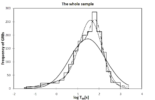
Figure 1: Fitting of the $\log T_{90}$ histogram in the whole sample with 15 bins (fit No.VI.). The number of GRBs per bin is given by the product of the frequency and width. (There are two equally populated bins between $-0.74<\log T_{90}<0.14$ divided at $\log T_{90}=-0.30$. For these bins the frequencies are 20.45, and hence the number of GRBs in these bins equal to $20.45\times 0.44=9$.) The theoretical curves show the best fits: full line = 1 Gaussian curve; dotted line = sum of 2 Gaussian curves; dash-dotted line = sum of 3 Gaussian curves.

We also performed the fitting with the sum of three Gaussian curves (eight parameters: three means, three standard deviations and two independent weights), and obtained an excellent fit with $\chi_{3}^{2}=2.4$ for fit No.VI, because the goodness-of-fit gives for dof = 15 - 8 - 1 = 6 the significance level is 88.2%. The best fitted curve is also seen on Fig. 1 showing even better correspondence with the measured data. The same excellent fits are obtained also for the remaining six binnings.

The key question here is following: Is the decreasing $\Delta\chi^{2}=7.5-2.4=5.1$ statistically significant? To answer this question we proceed similarly to Horváth (1998) and used the test proposed by Band et al. (1997) in Appendix A. The significance level from the F-test is 3.63%. This implies that the rejection of the null-hypothesis (i.e. that the sum of the two Gaussian curves is enough) is adequate, because the probability of the mistake for this rejection is not higher than 3.63%. We arrive into a conclusion that the strengthening of $\chi^{2}$ need not be a fluctuation. Similar results are obtained for the remaining six fits - only for the fit No.VII the significance is just above the usual 5% limit. (The significances smaller than 5% are denoted by boldface.) In other words, the introduction of the third subgroup - purely from the statistical point of view - is significant in six fits from the done seven ones. Note that the same F-test can be applied also for the difference $\chi_{1}^{2}-\chi_{2}^{2}$, and we always obtain the conclusion that the introduction of the second subgroup - instead of the one single group - is strongly supported.

3.2 The sample with $z$

Table 2: Results of the $\chi^{2}$ fitting of the sample with the known redshift with 130 GRBs.

$$\begin{array}[]{lrrrrrrr}\hline\cr Fit&I.&II.&III.&IV.&V.&VI.&VII.\\ No.\,of&&&&&&&\\ bins&10&11&12&15&16&17a&17b\\ \hline\cr 1G&&&&&&&\\ \chi_{1}^{2}&9.7&12.2&13.9&11.8&14.8&16.8&11.9\\ si.[\%]&20.9&14.4&12.6&46.0&31.8&26.5&61.2\\ \mu&1.55&1.52&1.53&1.69&1.54&1.54&1.53\\ \sigma&0.74&0.77&0.74&0.78&0.76&0.75&0.76\\ \hline\cr 2G&&&&\\ \chi_{2}^{2}&2.6&6.7&7.7&4.7&7.9&10.1&5.3\\ si.[\%]&62.4&24.0&26.0&86.0&64.0&51.8&91.8\\ \mu_{1}&1.47&-0.50&0.17&0.22&0.70&-0.69&-0.66\\ \sigma_{1}&0.77&1.00&0.88&0.94&0.86&0.10&0.15\\ \mu_{2}&1.97&1.58&1.62&1.77&1.68&1.59&1.58\\ \sigma_{2}&0.10&0.63&0.58&0.60&0.55&0.62&0.63\\ w_{2}&0.12&0.97&0.91&0.91&0.82&0.97&0.97\\ F[\%]&6.97&28.21&22.19&{\bf 2.20}&6.50&9.74&{\bf 1.70}\\ \hline\cr 3G&&&&\\ \chi_{3}^{2}&2.0&2.0&1.9&2.2&4.0&5.4&2.8\\ si.[\%]&15.4&49.8&59.1&89.9&77.8&71.4&94.8\\ \mu_{1}&1.04&-0.13&1.16&0.17&1.07&-0.57&-0.12\\ \sigma_{1}&0.30&1.00&1.05&0.50&0.92&0.05&0.14\\ \mu_{2}&1.17&0.94&1.61&1.14&1.32&1.12&0.95\\ \sigma_{2}&1.10&0.26&0.25&0.26&0.12&0.42&0.33\\ w_{2}&0.25&0.24&0.53&0.24&0.49&0.48&0.28\\ \mu_{3}&1.94&1.85&1.91&2.00&1.88&2.00&1.86\\ \sigma_{3}&0.34&0.44&0.18&0.43&0.33&0.34&0.43\\ w_{3}&0.49&0.69&0.25&0.67&0.41&0.49&0.67\\ F[\%]&89.64&24.41&10.51&13.29&12.66&11.40&10.96\\ \hline\cr\end{array}$$

The sample contains 130 events with duration informations. Also here we performed seven fits, but now the number of bins needed to be smaller due to the smaller number of objects in the sample. Again we did different binnings - fits VI. and VII. had 17 bins, but the structure was different. In each bin again the number of GRBs was higher than 5. The results are collected in Table 2., and fit No.II. is shown on Fig. 2.

Here the results, compared with the whole sample, are different from two reasons. First, here the fittings with one single Gaussian curve are also acceptable, and only for two fits the F-test show that the introduction of the second subgroup is adequate. Second, the introduction of the third subgroup is not needed from the F-test. All this shows that this sample can be defined by one single group, and even the separation into the short-long GRBs is not needed.

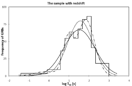
Figure 2: Fitting of $\log T_{90}$ in the sample with known redshifts. The theoretical curves show the best fits. The notation of the lines is the same as in Fig.1.

3.3 The sample without $z$

Table 3: Results of the $\chi^{2}$ fitting of the sample without the known redshift with 258 GRBs.

$$\begin{array}[]{lrrrrrrr}\hline\cr Fit&I.&II.&III.&IV.&V.&VI.&VII.\\ No.\,of&&&&&&&\\ bins&11&14&16&18&20&22&23\\ \hline\cr 1G&&&&&&&\\ \chi_{1}^{2}&57.8&66.8&67.3&71.4&76.0&83.8&76.2\\ si.[\%]&10^{-7}&10^{-8}&10^{-7}&10^{-7}&10^{-7}&10^{-8}&10^{-6}\\ \mu&1.47&1.41&1.41&1.41&1.41&1.42&1.41\\ \sigma&0.83&0.90&0.86&0.90&0.87&0.90&0.88\\ \hline\cr 2G&&&&\\ \chi_{2}^{2}&6.9&9.5&15.1&13.7&18.2&23.2&19.5\\ si.[\%]&22.8&30.6&13.0&31.8&20.0&10.9&30.0\\ \mu_{1}&-0.04&0.09&0.36&0.22&0.38&0.28&0.48\\ \sigma_{1}&0.81&1.07&0.98&1.06&1.00&1.03&1.03\\ \mu_{2}&1.58&1.60&1.60&1.61&1.62&1.62&1.63\\ \sigma_{2}&0.51&0.51&0.49&0.50&0.48&0.49&0.48\\ w_{2}&0.86&0.83&0.80&0.81&0.79&0.80&0.76\\ F[\%]&0.36&0.04&0.07&0.01&0.01&0.01&10^{-3}\\ \hline\cr 3G&&&&\\ \chi_{3}^{2}&2.9&3.1&10.6&9.2&14.8&18.3&17.0\\ si.[\%]&23.3&68.2&15.8&42.1&19.1&14.5&25.9\\ \mu_{1}&-0.46&-0.55&-0.52&-0.38&0.97&-0.38&-0.12\\ \sigma_{1}&0.40&0.82&0.59&0.80&1.13&0.78&0.86\\ \mu_{2}&0.86&1.47&1.37&1.51&1.15&1.48&1.52\\ \sigma_{2}&0.33&0.56&0.57&0.57&0.19&0.56&0.55\\ w_{2}&0.20&0.77&0.67&0.78&0.17&0.74&0.74\\ \mu_{3}&1.72&1.97&1.89&1.91&1.82&1.94&1.88\\ \sigma_{3}&0.43&0.15&0.28&0.15&0.29&0.20&0.20\\ w_{3}&0.72&0.13&0.25&0.11&0.45&0.15&0.13\\ F[\%]&40.20&6.81&39.50&23.87&47.00&33.60&53.60\\ \hline\cr\end{array}$$

Here the sample contains 258 events with duration information. Also here we did seven fits with different binnings. In each bin again the number of GRBs was higher than 5. The results are collected in Table 3., and fit No.I. is shown on Fig. 3.

The results, compared with the whole sample, are similar - except for one thing: The introduction of the third subgroup is not needed from the F-test. All this shows that this sample can well be defined by the sum of two and only two subgroups.

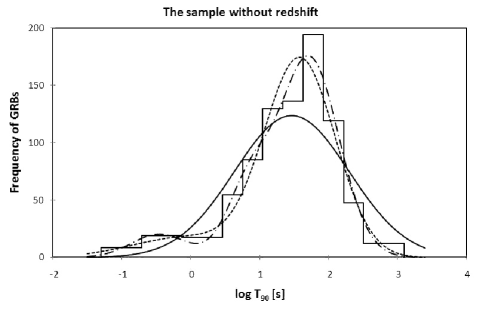
Figure 3: Fitting of $\log T_{90}$ in the sample with unknown redshifts. The theoretical curves show the best fits. The notation of the lines is the same as in Fig.1.

4 Discussion of the results

To discuss the results, first of all, we should recognize that we have proven the existence of the short and long subgroups also in the Swift data-set. Both the whole sample and the sample with no redshifts, respectively, contain these two subgroups, because the fits with one single Gaussian curve are fully wrong. It is also highly remarkable that also the weight of the short subgroup is in accordance with the expectation. As it follows from Horváth et al. (2006), in the BATSE Catalog the populations of the short, intermediate and long bursts are roughly in the ratio 20:10:70. Nevertheless, because the short bursts are harder and Swift is more sensitive to softer GRBs, one may expect that in the Swift database the population of short GRBs should be comparable or smaller than 20% due to instrumental reasons. The obtained weights for the whole sample (being between 10 and 26%) are in accordance with this expectation. Also the other values of the best parameters - i.e. two means and two standard deviations - are roughly in the ranges that can be expected from the BATSE values. The differences can be given by the different instrumentations. For example, the mean values of the $\log T_{90}$ should be slightly longer in the Swift database compared with the BATSE data (Barthelmy et al. (2005), Band (2006)). In Horváth (1998) the BATSE’s means are -0.35 (short) and 1.52 (long), respectively. Here we obtained for the whole sample values from -0.01 to 0.91 (short) and from 1.60 to 1.94 (long), respectively. All this implies that - concerning the short and long GRBs - the situation is in essence identical to the BATSE data-set.

For the sample with known redshifts the situation is different, because the fittings still allow one single Gaussian curve. This result can be easily explained by selection effects - it is well-known that the observational determination of the redshifts in the Swift data sample is easier for the long bursts due to observational strategies (simply, it is more complicated to detect and to follow the afterglows of short GRBs (Gehrels et al. (2005))).

Concerning the third intermediate subgroup the whole sample also supports its existence; from seven tests six ones gave significances below $5\%$. Hence, strictly speaking, the third subclass does exist and the probability of the mistake for this claim is not higher than x %, where $2.52<x<5.41$. This result is in accordance with the expectation, once a comparison with the BATSE database is provided. As it was said in Introduction, for the BATSE database the first evidence of third subgroup came from this $\chi^{2}$ method, and hence also for the Swift database this test should give positive support for this subgroup, if the two datasets are comparable. It is the key result of this article that this expectation is fulfilled. Our study has shown that the classical $\chi^{2}$ fitting - in combination with F-test - may well work also in the Swift database (similarly to the BATSE database (Horváth (1998))).

Horváth et al. (2008) confirmed the third subgroup in the Swift dataset by the maximum likelihood (ML) method. Our significance between 2.52% and 5.41% is weaker than the 0.46% significance obtained by Horváth et al. (2008), which is expectable, because the ML method is a stronger statistical test. This is seen from new two studies, too: the ML test on the databases of RHESSI (Řípa et al. (2009)) and BeppoSAX (Horváth (2009)) satellites, respectively, confirmed the existence of the third intermediate sublass; on the other hand, the $\chi^{2}$ test either did not give a high enough significance for RHESSI data (Řípa et al. (2009)) or was not used for BeppoSAX data at all (Horváth (2009)).

It can also be expected that the mean $\log T_{90}$ for the intermediate group should be much higher in the Swift database due to the different redshift distributions (Band (2006); Jakobsson et al. (2006); Bagoly et al. (2006)). The mean value for the BATSE’s intermediate subgroup is 0.64 (Horváth (1998)), but here the value is between 1.02 and 1.64. Also Horváth et al. (2008) obtained a similar value (1.107). Hence, also the typical durations are in accordance with the expectations.

The sample with no redshift did not find the third subgroup. This result can be explained by the smaller number of objects in the sample. The sample with known redshifts is strongly biased by selection effects, and here even the existence of the short subgroup was in doubt - hence, it seems to be hopeless to obtain some conclusions concerning the third subgroup.

5 Conclusions

Since the $\chi^{2}$ fitting of the GRB duration distribution and the F-test were successfully used in the work Horváth (1998) (presenting the first evidence of the existence of three GRB subgroups), we proceed identically, but with the Swift’s data.

The results may be summarized in the following four points:

1. Concerning the short and long subgroups all is in accordance with the expectation: they are detected also in the Swift database and - in addition - in the Swift database the weight of the short subgroup is smaller, which can be well explained by the Swift’s higher effective sensitivity to the softer bursts.

2. The whole sample of 388 objects gives support for three subgroups, because from seven fittings of the whole sample six ones confirmed the existence of the intermediate subgroup on a smaller than 5% significance level. Hence, concerning the Swift database, the situation is similar to the BATSE dataset - although our signficances are weaker than $>0.02\%$ of Horváth (1998).

3. The samples with and without known redshifts separately are either not enough populated, or strongly biased. Hence, no far reaching conclusions can be drawn from them.

4. Similarly to the BATSE database, here it is shown again that the classical $\chi^{2}$ test - in combination with F-test - is also effective for the Swift GRB sample.

Table 4: Swift GRBs with no measured redshifts; Part I.

$$\begin{array}[]{lrrr}\hline\cr GRB&T_{90}&fluence&peak-flux\\ &sec&10^{-7}\,erg/cm^{2}&ph/(cm^{2}sec)\\ \hline\cr 090201&83.0&300.00&14.70\\ 090129&17.5&21.00&3.70\\ 090123&131.0&29.00&1.70\\ 090118&16.0&4.00&n/a\\ 090113&9.1&7.60&2.50\\ 090111&24.8&6.20&0.90\\ 090107A&12.2&2.30&1.10\\ 081230&60.7&8.20&0.70\\ 081228&3.0&0.89&0.60\\ 081226A&0.4&0.99&2.40\\ 081221&34.0&181.00&18.20\\ 081211A&3.5&1.30&0.80\\ 081210&146.0&18.00&2.50\\ 081203B&23.4&21.00&n/a\\ 081128&100.0&23.00&1.30\\ 081127&37.0&4.90&0.60\\ 081126&54.0&33.00&3.70\\ 081109A&190.0&36.00&1.10\\ 081104&59.1&20.00&1.00\\ 081102&63.0&23.00&1.40\\ 081101&0.2&0.62&3.60\\ 081025&23.0&19.00&1.30\\ 081024A&1.8&1.20&1.10\\ 081022&160.0&25.00&0.60\\ 081017&320.0&14.00&0.07\\ 081016B&2.6&0.99&0.50\\ 081012&29.0&11.00&1.00\\ 081011&9.0&1.60&0.40\\ 080919&0.6&0.72&1.20\\ 080916B&32.0&6.30&0.60\\ 080915B&3.9&9.90&8.50\\ 080915A&14.0&2.30&0.50\\ 080905A&1.0&1.40&1.30\\ 080903&66.0&14.00&0.80\\ 080822B&64.0&1.70&0.06\\ 080802&176.0&13.00&0.30\\ 080727C&79.7&52.00&2.30\\ 080727B&8.6&31.00&7.60\\ 080727A&4.9&1.30&0.30\\ 080725&120.0&37.00&2.30\\ 080723A&17.3&3.30&0.90\\ 080714&33.0&25.00&4.20\\ 080703&3.4&2.00&1.00\\ 080702B&20.0&5.00&0.50\\ 080702A&0.5&0.36&0.70\\ 080701&18.0&7.10&2.20\\ \hline\cr\end{array}$$

Table 5: Swift GRBs with no measured redshifts; Part II.

$$\begin{array}[]{lrrr}\hline\cr GRB&T_{90}&fluence&peak-flux\\ &sec&10^{-7}\,erg/cm^{2}&ph/(cm^{2}sec)\\ \hline\cr 080623&15.2&10.00&2.00\\ 080613B&105.0&58.00&2.70\\ 080602&74.0&32.00&2.90\\ 080524&9.0&2.90&0.40\\ 080523&102.0&8.80&0.50\\ 080517&64.6&5.60&0.60\\ 080515&21.0&20.00&3.90\\ 080506&150.0&13.00&0.40\\ 080503&170.0&20.00&0.90\\ 080426&1.7&3.70&4.80\\ 080409&20.2&6.10&3.70\\ 080405&40.0&12.00&n/a\\ 080328&90.6&94.00&5.50\\ 080325&128.4&49.00&1.40\\ 080320&14.0&2.70&0.60\\ 080319D&24.0&3.20&0.10\\ 080319A&64.0&48.00&1.20\\ 080315&65.0&1.40&0.04\\ 080307&125.9&8.70&0.40\\ 080303&67.0&6.60&1.40\\ 080229A&64.0&90.00&5.70\\ 080218B&6.2&5.10&3.10\\ 080218A&27.6&6.30&1.40\\ 080212&123.0&29.00&1.20\\ 080207&340.0&61.00&1.00\\ 080205&106.5&21.00&1.40\\ 080130&65.0&7.70&0.20\\ 080129&48.0&8.90&0.20\\ 080123&115.0&5.70&1.80\\ 080121&0.7&0.30&n/a\\ 071129&420.0&35.00&0.90\\ 071118&71.0&5.00&0.30\\ 071112B&0.3&0.48&1.30\\ 07110&19.0&0.76&0.40\\ 071028B&55.0&2.50&1.40\\ 071028A&27.0&3.00&0.30\\ 071025&109.0&65.00&1.60\\ 071018&376.0&10.00&0.20\\ 071013&26.0&3.20&0.40\\ 071011&61.0&22.00&1.70\\ 071008&18.0&2.40&0.50\\ 071006&50.0&1.40&13.00\\ 071001&58.5&7.70&0.90\\ 070923&0.1&0.10&2.40\\ 070920B&20.2&6.60&0.80\\ 070920A&56.0&5.10&0.30\\ 070917&7.3&20.00&8.50\\ 070913&3.2&2.50&1.40\\ 070911&162.0&120.00&3.90\\ \hline\cr\end{array}$$

Table 6: Swift GRBs with no measured redshifts; Part III.

$$\begin{array}[]{lrrr}\hline\cr GRB&T_{90}&fluence&peak-flux\\ &sec&10^{-7}\,erg/cm^{2}&ph/(cm^{2}sec)\\ \hline\cr 070810B&80.0&0.12&1.80\\ 070809&1.3&1.00&1.20\\ 070808&32.0&12.00&2.00\\ 070805&31.0&7.20&0.70\\ 070731&2.9&1.60&1.20\\ 070729&0.9&1.00&1.00\\ 070721A&3.4&0.71&0.70\\ 070714A&2.0&1.50&1.80\\ 070704&380.0&59.00&2.10\\ 070628&39.1&35.00&5.10\\ 070621&33.3&43.00&2.50\\ 070616&402.0&192.00&1.90\\ 070612B&13.5&17.00&2.60\\ 070610&4.6&2.40&0.90\\ 070531&44.0&11.00&1.00\\ 070520B&66.0&9.20&0.40\\ 070520A&18.0&2.50&0.40\\ 070518&5.5&1.60&0.70\\ 070517&9.0&2.60&0.80\\ 070509&7.7&1.70&0.70\\ 070429B&0.5&0.63&1.80\\ 070429A&163.0&9.20&0.40\\ 070427&11.0&7.20&1.30\\ 070420&77.0&140.00&7.10\\ 070419B&236.5&75.00&1.40\\ 070412&34.0&4.80&0.70\\ 070406&0.7&0.45&0.70\\ 070330&9.0&1.80&0.90\\ 070328&69.0&89.00&4.20\\ 070227&7.0&16.00&2.70\\ 070224&34.0&3.10&0.30\\ 070223&89.0&17.00&0.70\\ 070220&129.0&106.00&5.88\\ 070219&17.0&3.20&0.70\\ 070209&0.1&0.11&2.40\\ 070129&460.0&31.00&0.60\\ 070126&51.0&1.60&0.20\\ 070103&19.0&3.40&1.10\\ 061222A&72.0&83.00&9.20\\ 061218&4.1&0.20&0.41\\ 061202&91.0&35.00&2.60\\ 061126&191.0&72.00&9.80\\ 061102&17.6&1.90&0.20\\ 061028&106.0&9.70&0.70\\ 061027&150.0&4.70&0.08\\ 061021&46.0&30.00&6.10\\ 061019&191.0&17.00&2.20\\ 061006&130.0&14.30&5.36\\ 061004&6.2&5.70&2.50\\ 061002&17.6&6.80&0.80\\ 060929&12.4&2.80&0.40\\ 060923C&76.0&16.00&1.00\\ 060923B&8.8&4.80&1.50\\ 060923A&51.7&8.70&1.30\\ 060919&9.1&5.50&2.20\\ 060904A&80.0&79.00&4.90\\ \hline\cr\end{array}$$

Table 7: Swift GRBs with no measured redshifts; Part IV.

$$\begin{array}[]{lrrr}\hline\cr GRB&T_{90}&fluence&peak-flux\\ &sec&10^{-7}\,erg/cm^{2}&ph/(cm^{2}sec)\\ \hline\cr 060825&8.1&9.80&2.70\\ 060813&14.9&55.00&9.00\\ 060807&34.0&7.30&0.80\\ 060805&5.4&0.74&0.30\\ 060804&16.0&5.10&1.20\\ 060801&0.5&0.81&1.30\\ 060728&60.0&2.40&n/a\\ 060719&55.0&16.00&2.30\\ 060717&3.0&0.65&0.50\\ 060712&26.0&13.00&1.70\\ 060607B&31.0&17.00&1.50\\ 060602A&60.0&16.00&0.50\\ 060516&160.0&11.00&0.30\\ 060515&52.0&14.00&0.80\\ 060510A&21.0&98.00&17.00\\ 060507&185.0&45.00&1.30\\ 060501&26.0&12.00&1.90\\ 060428B&58.0&7.20&0.60\\ 060428A&39.4&14.00&2.40\\ 060427&64.0&5.00&0.30\\ 060424&37.0&6.80&1.60\\ 060421&11.0&12.00&3.00\\ 0604131&50.0&36.00&0.90\\ 060403&30.0&14.00&1.00\\ 060323&18.0&5.70&0.80\\ 060322&213.0&51.00&2.10\\ 060319&12.0&2.70&1.10\\ 060313&0.7&11.30&12.10\\ 060312&43.0&18.00&1.50\\ 060306&61.0&22.00&6.10\\ 060223B&10.2&16.00&2.90\\ 060219&62.0&4.20&0.60\\ 060211B&29.0&4.70&0.70\\ 060211A&126.0&15.00&0.40\\ 060204B&134.0&30.00&1.30\\ 060203&60.0&8.50&0.60\\ 060202&203.7&24.00&0.50\\ 060117&16.0&204.00&48.90\\ 060111B&59.0&16.00&1.40\\ 060111A&13.0&11.80&1.72\\ 060110&17.0&14.00&1.90\\ 060109&116.0&6.40&0.50\\ 060105&55.0&182.00&7.50\\ 060102&21.0&2.40&0.40\\ 051227&8.0&2.30&0.97\\ 051221B&61.0&11.30&0.54\\ 051213&70.0&8.00&0.51\\ 051210&1.4&0.83&0.75\\ 051117B&8.0&1.40&0.46\\ 051117A&140.0&46.00&0.93\\ 051114&2.2&1.32&0.73\\ 051113&94.0&26.00&2.40\\ 051105A&0.3&0.20&2.00\\ 051021B&47.0&9.10&0.63\\ 051016A&22.0&8.80&1.60\\ 051012&13.0&2.90&0.60\\ 051008&16.0&58.00&5.50\\ 051006&26.0&12.80&1.90\\ 051001&190.0&18.00&0.51\\ \hline\cr\end{array}$$

Table 8: Swift GRBs with no measured redshifts; Part V.

$$\begin{array}[]{lrrr}\hline\cr GRB&T_{90}&fluence&peak-flux\\ &sec&10^{-7}\,erg/cm^{2}&ph/(cm^{2}sec)\\ \hline\cr 050925&0.1&0.75&1.50\\ 050922B&250.0&26.00&1.02\\ 050916&90.0&11.00&0.69\\ 050915B&40.0&34.00&2.34\\ 050915A&53.0&8.80&0.80\\ 050911&16.0&3.01&1.31\\ 050906&0.1&0.07&1.15\\ 050827&49.0&21.20&1.86\\ 050822&102.0&26.10&2.47\\ 050820B&13.0&21.20&4.06\\ 050819&36.0&3.52&0.39\\ 050815&2.8&0.92&0.56\\ 050801&20.0&3.12&1.47\\ 050721&39.0&30.80&3.08\\ 050717&86.0&61.70&6.34\\ 050715&52.0&14.40&1.07\\ 050713A&70.0&52.50&4.78\\ 050712&48.0&11.00&0.55\\ 050701&22.0&13.60&2.77\\ 050607&26.5&6.05&0.99\\ 050528&10.8&4.40&1.23\\ 050509A&11.6&3.38&0.88\\ 050502B&17.5&4.72&1.43\\ 050422&59.2&6.15&0.57\\ 050421&10.3&1.18&0.44\\ 050418&83.0&53.90&3.80\\ 050416B&5.4&11.30&5.85\\ 050412&26.0&5.66&0.49\\ 050410&43.0&43.00&1.80\\ 050326&29.5&90.50&12.40\\ 050306&160.0&120.00&3.64\\ 050219B&27.0&164.00&25.40\\ 050219A&23.0&42.10&3.61\\ 050215B&8.0&2.33&0.68\\ 050215A&6.0&7.29&0.51\\ 050202&0.1&0.33&2.98\\ 050128&13.8&51.70&7.59\\ 050124&4.1&12.30&5.57\\ 050117&169.0&91.20&2.40\\ 041228&62.0&36.10&1.65\\ 041226&15.0&3.23&0.34\\ 041224&235.0&75.30&2.95\\ 041223&107.0&171.00&7.49\\ 041220&5.0&3.82&1.83\\ 041219C&40.0&20.00&1.50\\ 041219B&30.0&n/a&10.00\\ 041219A&520.0&1000.00&25.00\\ 041217&7.5&65.70&4.40\\ \hline\cr\end{array}$$

Table 9: Swift GRBs with known redshifts; Part I.

$$\begin{array}[]{lrrrr}\hline\cr GRB&T_{90}&fluence&peak-flux&z\\ &sec&10^{-7}\,erg/cm^{2}&ph/(cm^{2}sec)&\\ \hline\cr 090205&8.8&1.90&0.50&4.6749\\ 090102&27.0&0.68&5.50&1.5477\\ 081222&24.0&48.00&7.70&2.7467\\ 081203A&294.0&77.00&2.90&2.1000\\ 081121&14.0&41.00&4.40&2.5120\\ 081118&67.0&12.00&0.60&2.5800\\ 081029&270.0&21.00&0.50&3.8474\\ 081028A&260.0&37.00&0.50&3.03800\\ 081008&185.5&43.00&1.30&1.96775\\ 081007&10.0&7.10&2.60&0.52950\\ 080928&280.0&25.00&2.10&1.6910\\ 080916A&60.0&40.00&2.70&0.68900\\ 080913&8.0&5.60&1.40&6.57000\\ 080906&147.0&35.00&1.00&2.00000\\ 080905B&128.0&18.00&0.50&2.37400\\ 080810&106.0&46.00&2.00&3.35000\\ 080805&78.0&25.00&1.10&1.50500\\ 080804&34.0&36.00&3.10&2.20225\\ 080721&16.2&120.00&20.90&2.59650\\ 080710&120.0&14.00&1.00&0.84500\\ 080707&27.1&5.20&1.00&1.23000\\ 080607&79.0&240.00&23.10&3.03600\\ 080605&20.0&133.00&19.90&1.63980\\ 080604&82.0&8.00&0.40&1.41600\\ 080603B&60.0&24.00&3.50&2.69000\\ 080520&2.8&0.55&0.50&1.54500\\ 080516&5.8&2.60&1.80&3.20000\\ 080430&16.2&12.00&2.60&0.75850\\ 080413B&8.0&32.00&18.70&1.10000\\ 080413A&46.0&35.00&5.60&2.43300\\ 080411&56.0&264.00&43.20&1.03000\\ 080330&61.0&3.40&0.90&1.51000\\ 080319C&34.0&36.00&5.20&1.95000\\ 080319B&50.0&810.00&24.80&0.93700\\ 080310&365.0&23.00&1.30&2.42580\\ 080210&45.0&18.00&1.60&2.64100\\ \hline\cr\end{array}$$

Table 10: Swift GRBs with known redshifts; Part II.

$$\begin{array}[]{lrrrr}\hline\cr GRB&T_{90}&fluence&peak-flux&z\\ &sec&10^{-7}\,erg/cm^{2}&ph/(cm^{2}sec)&\\ \hline\cr 071227&1.8&2.20&1.60&0.3835\\ 071122&68.7&5.80&0.40&1.14\\ 071117&6.6&24.00&11.30&1.331\\ 071112C&15.0&30.00&8.00&0.82\\ 071031&180.0&9.00&0.50&2.692\\ 071021&225.0&13.00&0.70&5.0\\ 071020&4.2&23.00&8.40&2.1435\\ 071010B&35.7&44.00&7.70&0.947\\ 071010A&6.0&2.00&0.80&0.98\\ 071003&150.0&83.00&6.30&1.0185\\ 070810A&11.0&6.90&1.90&2.17\\ 070802&16.4&2.80&0.40&2.45\\ 070724A&0.4&0.80&1.00&0.457\\ 070721B&340.0&36.00&1.50&3.626\\ 070714B&64.0&7.20&2.70&0.92\\ 070612A&370.0&110.00&1.50&0.617\\ 070611&12.0&39.00&0.80&2.04\\ 070529&109.0&26.00&1.40&2.4996\\ 070521&37.9&80.00&6.70&0.553\\ 070508&21.0&200.00&24.70&0.82\\ 070506&4.3&2.10&1.00&2.31\\ 070419A&116.0&5.60&2.80&0.97\\ 070411&101.0&25.00&1.00&2.954\\ 070318&63.0&23.00&1.60&0.838\\ 070306&210.0&55.00&4.20&1.497\\ 070208&48.0&4.30&0.90&1.165\\ 070110&85.0&16.00&0.60&2.352\\ 061222B&40.0&22.00&1.50&3.355\\ 061217&0.3&0.46&1.30&0.827\\ 061210&85.0&11.00&5.30&0.41\\ 061201&0.8&3.30&3.90&0.111\\ 061121&81.0&137.00&21.10&1.314\\ 061110B&128.0&13.00&0.40&3.44\\ 061110A&41.0&11.00&0.50&0.758\\ 061007&75.0&450.00&15.30&1.2615\\ 060927&22.6&11.00&2.80&5.6\\ 060926&8.0&2.20&1.10&3.208\\ 060912&5.0&13.00&8.50&0.937\\ 060908&19.3&29.00&3.20&2.43\\ 060906&43.6&22.10&2.00&3.685\\ 060904B&192.0&17.00&2.50&0.703\\ 060814&146.0&150.00&7.40&0.84\\ 060729&116.0&27.00&1.40&0.54\\ 060714&115.0&30.00&1.40&2.71\\ 060708&9.8&5.00&2.00&2.3\\ 060707&68.0&17.00&1.10&3.43\\ \hline\cr\end{array}$$

Table 11: Swift GRBs with known redshifts; Part III.

$$\begin{array}[]{lrrrr}\hline\cr GRB&T_{90}&fluence&peak-flux&z\\ &sec&10^{-7}\,erg/cm^{2}&ph/(cm^{2}sec)&\\ \hline\cr 060614&102.0&217.00&11.60&0.1275\\ 060607A&100.0&26.00&1.40&3.082\\ 060605&15.0&4.60&0.50&3.76\\ 060604&10.0&1.30&0.60&2.68\\ 060526&13.8&4.90&1.70&3.21\\ 060522&69.0&11.00&0.60&5.11\\ 060512&8.6&2.30&0.90&0.4428\\ 060510B&276.0&42.00&0.60&4.9\\ 060505&4.0&6.20&1.90&0.089\\ 060502B&90.0&0.40&4.40&0.287\\ 060502A&33.0&22.00&1.70&1.51\\ 060418&52.0&81.00&6.70&1.4895\\ 060223A&11.0&6.80&1.40&4.41\\ 060210&255.0&77.00&2.80&3.91\\ 060206&7.0&8.40&2.80&4.048\\ 060123&900.0&3.00&0.04&1.099\\ 060116&113.0&26.00&1.10&5.3\\ 060115&142.0&18.00&0.90&3.53\\ 060108&14.4&3.70&0.70&2.03\\ 051221A&1.4&11.60&12.10&0.547\\ 051111&47.0&39.00&2.50&1.549\\ 051109B&15.0&2.70&0.50&0.08\\ 051109A&36.0&21.00&3.70&2.346\\ 051016B&4.0&1.70&1.32&0.9364\\ 050922C&5.0&17.00&7.36&2.198\\ 050908&20.0&4.91&0.70&3.3459\\ 050904&225.0&50.70&0.66&6.29\\ 050826&35.0&4.51&0.43&0.297\\ 050824&25.0&2.92&0.52&0.83\\ 050820A&26.0&40.10&2.50&2.61335\\ 050814&65.0&18.30&0.75&5.3\\ 050813&0.6&0.43&0.92&1.80\\ 050803&85.0&22.30&1.08&0.422\\ 050802&13.0&22.00&2.65&1.71\\ 050730&155.0&24.20&0.57&3.9669\\ 050724&3.0&11.80&3.29&0.2575\\ 050603&13.0&76.30&27.60&2.821\\ 050525A&8.8&156.00&42.30&0.606\\ 050509B&0.04&0.13&1.33&0.225\\ 050505&60.0&24.90&1.81&4.27\\ 050416A&2.4&4.31&4.97&0.6535\\ 050406&3.0&0.81&0.38&2.44\\ 050401&33.0&85.50&12.60&2.9\\ 050319&10.0&6.25&1.45&3.24\\ 050318&32.0&13.10&3.20&1.44\\ 050315&96.0&32.30&1.98&1.949\\ 050223&23.0&6.40&0.70&0.58775\\ 050126&26.0&8.60&0.70&1.29\\ \hline\cr\end{array}$$

References

Bagoly et al. (1998) Bagoly, Z., Mészáros, A.,
Horváth, I., Balázs, L.G. & Mészáros, P. 1998, ApJ, 498, 342
Bagoly et al. (2003) Bagoly, Z., Csabai, I.,
Mészáros, A., Mészáros, P., Horváth, I.,
Balázs, L.G. & Vavrek I. 2003, A&A, 398, 919
Bagoly et al. (2006) Bagoly, Z., Mészáros, A.,
Balázs, L.G., Horváth, I., Klose, S.,
Larsson, S., Mészáros, P., Ryde, F., Tusnády 2006, A&A, 453, 797
Balázs et al. (2003)
Balázs, L.G., Bagoly, Z., Horváth, I., Mészáros, A. &
Mészáros, P. 2003, A&A, 401, 129