The consequences of finite-time proper orthogonal decomposition for an extensively chaotic flow field

Abstract

The use of proper orthogonal decomposition (POD) to explore the complex fluid flows that are common in engineering applications is increasing and has yielded new physical insights. However, for most engineering systems the dimension of the dynamics is expected to be very large yet the flow field data is available only for a finite time. In this context, it is important to establish the convergence of the POD in order to accurately estimate such quantities as the Karhunen-Loève dimension. Using direct numerical simulations of Rayleigh-Bénard convection in a finite cylindrical geometry we explore a regime exhibiting extensive chaos and demonstrate the consequences of performing a POD with a finite amount of data. In particular, we show that the convergence in time of the eigenvalue spectrum, the eigenfunctions, and the dimension are very slow in comparison with the time scale of the convection rolls and that the errors incurred by not using the asymptotic values can be significant. We compute the dimension using two approaches, the method of snapshots and a Fourier method that exploits the azimuthal symmetry. We find that the convergence rate of the Fourier method is vastly improved over the method of snapshots. The dimension is found to be extensive as the system size is increased and for a dimension measurement that captures 90% of the variance in the data the Karhunen-Loève dimension is about 20 times larger than the Lyapunov dimension.

1 Introduction

Many open challenges remain in the development of ways to describe, model, and predict chaotic fluid flows [1]. One method proposed by Lumley [2] to study turbulence is to use a Karhunen-Loève decomposition, or proper orthogonal decomposition (POD), to decompose the flow into an optimal set of basis functions. This has lead to many discoveries and has increased our understanding of turbulence including the dynamics of streaks and bursting events [3, 4, 5, 6, 7, 8, 9, 10, 11], the dynamics of energy transfer [12, 13], and the mechanism of drag reduction [14, 15]. Recently, this has been extended to many experimental and numerical investigations of more complicated flow fields in engineering applications that are quite different than a typical theoretical investigation of fluid turbulence (c.f. [16, 17]). An important difference is that the interval of time over which the data is available is often very short. This limiting factor is present in both experimental and numerical studies. It is anticipated that the dimension describing the dynamics of these systems is very large and as a result the short time observations provide only a limited sample of the overall dynamics.

We explore this by quantifying the convergence of the Karhunen-Loève dimension with time for a high-dimensional fluid flow field. Our results provide insights for the use of POD for more complex engineering flow fields where only a finite amount of data is available. Our results show that (i) the eigenvalue spectrum, the eigenfunctions, and the dimension for the POD of a complex flow field can be approximated from finite time observations; and (ii) tailoring the numerical algorithm to exploit the rotational invariance in the problem vastly improves the rate of convergence.

We show this by numerically integrating the time-dependent and three-dimensional Boussinesq equations that govern the fluid motion of Rayleigh-Bénard convection in a shallow cylindrical domain. In particular, we explore the spatiotemporal chaos of the fluid convection rolls that arise when a layer of fluid is heated uniformly from below in a gravitational field. A typical flow field pattern from our numerical simulations is shown in Fig. 1 which illustrates a horizontal mid-plane slice of the domain where red is hot rising fluid and blue is cool falling fluid.

The dimension of the attractor describing the dynamics of chaotic convection is expected to be much lower than one would find in fully developed turbulent flow [1, 18, 19]. However, the dimension of convection is large enough to test these ideas [19]. Our results provide quantitative estimates for the convergence rates and magnitudes of important diagnostics that result from a POD study.

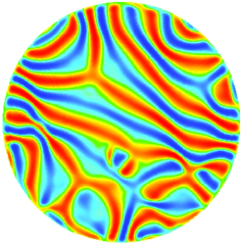
Figure 1: (color) A typical pattern of convection rolls from a numerical simulation of chaotic Rayleigh-Bénard convection in a shallow cylindrical domain. The flow field is shown at mid-depth $z=1/2$ where red indicates warm rising fluid and blue indicates cool falling fluid. For this simulation $\Gamma=10$, $R/R_{c}=3.5$, and $\sigma=1$.

2 Numerical Methods

2.1 Direct Numerical Simulation

The fluid motion of Rayleigh-Bénard convection is governed by the Boussinesq equations

$$\mathrm{\sigma}^{-1}\left(\partial_{t}+\mathbf{u}\cdot\mathbf{\nabla}\right)\mathbf{u}\! = \!-\nabla P+\nabla^{2}\mathbf{u}+\mathrm{R}T\hat{z},$$ (1)

$$\left(\partial_{t}+\mathbf{u}\cdot\mathbf{\nabla}\right)T = \nabla^{2}T,$$ (2)

$$\mathbf{\nabla}\cdot\mathbf{u} = 0,$$ (3)

which represent the conservation of momentum, energy, and mass. In our notation $\partial_{t}$ is a time derivative, $\hat{z}$ is a unit vector in the direction opposing gravity, $\mathbf{u}$ is the fluid velocity, $p$ is the pressure, and $T$ is the temperature. The equations are nondimensionalized using the layer depth $d$ as the length scale, the vertical diffusion time of heat $\tau_{v}=d^{2}/\alpha$ for the time scale where $\alpha$ is the thermal diffusivity, and the constant temperature difference $\Delta T$ between the bottom and top plates as the temperature scale. In our investigation we consider a shallow cylindrical convection domain of radius $r_{0}$ and depth $d$. On all material walls we impose the no-slip boundary condition

$$\mathbf{u}=0.$$ (4)

The top and bottom plates are held at a constant temperature $T(z=0)=1$ and $T(z=1)=0$ and the lateral sidewalls of the domain are perfectly conducting boundaries with

$$T=1-z.$$ (5)

There are three important nondimensional parameters that completely describe the dynamics. The aspect ratio of the domain

$$\Gamma=\frac{r_{0}}{d}$$ (6)

which is a measure of the system size and $r_{0}$ is the radius of the domain. The Prandtl number

$$\sigma=\frac{\nu}{\alpha}$$ (7)

where $\nu$ is the kinematic viscosity, and the Rayleigh number

$$R=\frac{g\beta\Delta Td^{3}}{\alpha\nu}$$ (8)

where $g$ is the acceleration due to gravity and $\beta$ is the coefficient of thermal expansion.

The control parameter that is varied in most experiments is $R$ [20]. For no-slip boundaries the critical value of the Rayleigh number is $R_{c}=1708$ which corresponds to the onset of convection rolls. For a fluid with $\sigma\approx 1$, as $R$ is increased $R\lesssim 10^{4}$ the steady convection rolls are replaced by patterns of rolls with time dependent dynamics that include periodic, quasiperiodic, and chaotic dynamics (c.f. [21, 22, 23, 24]). As $R$ is increased further $R\gtrsim 10^{5}$ the convection rolls are annihilated and replaced by thermal plume structures yielding turbulent convection [1]. In this paper we are interested in the range where the patterns of convection rolls exhibit spatiotemporal chaos and we use $R=6000$ (which yields $R/R_{c}=3.5$), $\sigma=1$ and a range of system sizes $6\leq\Gamma\leq 15$. In the following we solve the time-dependent Boussinesq equations using a geometrically flexible, efficient, spectral element algorithm [25, 26, 27]. Further details on the specific application of this numerical method to thermal convection can be found in Ref. [28].

2.2 Proper Orthogonal Decomposition

The POD of a fluid flow field can be cast as the solution of the Fredholm integral,

$$\int_{\Omega}K(\mathbf{x},\mathbf{x}^{\prime})\bm{\Phi}(\mathbf{x}^{\prime})d^{3}x^{\prime}=\mu\bm{\Phi}(\mathbf{x}),$$ (9)

where,

$$K(\mathbf{x},\mathbf{x^{\prime}})=\lim_{\tau\to\infty}\frac{1}{\tau}\int_{0}^{\tau}\mathbf{u}(\mathbf{x},t)\otimes\mathbf{u}(\mathbf{x}^{\prime},t)dt,$$ (10)

and $\otimes$ is an outer product, $\Omega$ is the volume of the entire domain, $\mathbf{x}$ is the position vector, $\bm{\Phi}(\mathbf{x})$ is the eigenvector with associated eigenvalue $\mu$, and $K(\mathbf{x},\mathbf{x}^{\prime})$ is the kernel. The kernel is built using the two-point correlation of the fluctuating space-time velocity components $\mathbf{u}(\mathbf{x},t)$ averaged over time $\tau$. The Karhunen-Loève dimension $D_{KL}$ is the number of eigenmodes necessary to capture a given fraction $f$ of the total variance of the data

$$\frac{\displaystyle\sum_{j=1}^{D_{KL}}\mu_{j}}{\displaystyle\sum_{j=1}^{\infty}\mu_{j}}=f$$ (11)

where a typical choice is $f=0.9$. The observation time $\tau$ should be long enough such that most of the dynamics on the attractor have been observed. In the limit $\tau\rightarrow\infty$ this is satisfied. However, for a finite amount of data it is desired that the data is sufficient for the dimension to have converged to a value close to its asymptotic value such that $D_{KL}\approx D_{\infty}$.

For the Rayleigh-Bénard convection studied here we perform a POD on the two-dimensional flow field pattern at the mid plane as shown in Fig. 1. The reason for this is two-fold. One, a typical experiment using shadowgraphy to measure the convective roll pattern would generate the same type of data. Second, it is expected that the convection rolls do not contain structure in the vertical direction that would have a significant impact upon the dimension. In collecting data for our POD we use images from the flow field separated in time by 5$\tau_{v}$ where the total duration of the numerical simulation depends upon the system size explored.

2.2.1 Fourier Method

The size of the eigenvalue problem to solve the Fredholm integral in Eq. (9) is large. Two methods that are used to reduce the computations are the Fourier method and the method of snapshots.

For a rotationally invariant system every rotation of the solution is also valid. The coefficients of the POD in the azimuthal direction are therefore those of a Fourier series [29]. When this invariance is built into the computational procedure we refer to this as the Fourier method. Therefore, the eigenmode for mode $m$,

$$\bm{\Phi}_{m}(r,\theta)=\bm{\Psi}_{n}^{q}(r)e^{in\theta}$$ (12)

is uniquely described with an azimuthal wavenumber $n$ and eigen number $q$. This reduces the computation of the Karhunen-Loève modes to

$$\int_{0}^{r_{0}}\mathcal{K}_{n}(r,r^{\prime})\bm{\Psi}_{n}(r^{\prime})r^{\prime}dr^{\prime}=\mu_{n}\bm{\Psi}_{n}(r),$$ (13)

where,

$$\mathcal{K}_{n}(r,r^{\prime})=\lim_{\tau\to\infty}\frac{1}{\tau}\int_{0}^{\tau}\hat{\mathbf{u}}_{n}(r,t)\otimes\hat{\mathbf{u}}_{n}^{\star}(r^{\prime},t)dt,$$ (14)

with $\star$ denoting the complex conjugate and the weight $r^{\prime}$ is present because the inner product is evaluated in polar-cylindrical coordinates $(r,\theta)$. The Fourier transform of the velocity in the azimuthal direction is $\hat{\mathbf{u}}_{n}(r,t)$. The kernel in Eq. (13) is Hermitian as it was in Eq. (9) and yields real and positive eigenvalues. Using a $Q$-point quadrature to solve Eq. (13) yields $3Q$ eigenvectors and corresponding eigenvalues in descending order for each azimuthal mode $n$, denoted with eigen number $q$. Physically, each eigenvector $\bm{\Psi}_{n}^{q}(r)e^{in\theta}$ represents a velocity field and the eigenvalue $\mu_{n}^{q}$ is the time averaged energy of that flow field.

2.2.2 Method of Snapshots

The method of snapshots recasts the eigenfunction in the Fredholm integral in Eq. (9) as a linear combination of the snapshots where

$$c(t)=\int_{\Omega}\mathbf{u}(\mathbf{x}^{\prime},t)\bm{\Phi}(\mathbf{x}^{\prime})d^{3}x^{\prime}$$ (15)

and Eq. (9) is then

$$\lim_{\tau\to\infty}\frac{1}{\tau}\int_{0}^{\tau}\mathbf{u}(\mathbf{x},t)c(t)dt=\lambda\bm{\Phi}(\mathbf{x}).$$ (16)

Multiplying both sides by $\mathbf{u}(\mathbf{x},t^{\prime})$ and integrating yields,

$$\lim_{\tau\to\infty}\frac{1}{\tau}\int_{0}^{\tau}c(t)\int_{\Omega}\mathbf{u}(\mathbf{x},t^{\prime})\mathbf{u}(\mathbf{x},t)d^{3}xdt=\lambda c(t^{\prime})$$ (17)

or,

$$\lim_{\tau\to\infty}\frac{1}{\tau}\int_{0}^{\tau}\left(\mathbf{u}(\mathbf{x},t^{\prime}),\mathbf{u}(\mathbf{x},t)\right)c(t)dt=\lambda c(t^{\prime})$$ (18)

where $(~{},~{})$ denotes an inner product over the domain $\Omega$. The resulting equation is now a Fredholm integral in time. In fluid dynamics this is more computationally tractable because there are typically fewer time observations (snapshots) than there are spatial observations (grid points).

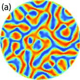
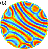
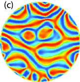
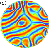
Figure 2: (color) Four flow fields from numerical simulation that are separated in time by $50\tau_{v}$ for $\Gamma=10$, $R/R_{c}=3.5$, $\sigma=1$. The values of $D_{KL}$ computed using the Fourier method for each individual flow field are 46.1, 46.8, 49.8, and 48.5 for panels (a)-(d) respectively.

Table 1: The cumulative Karhunen-Loève dimension of the four flow field images shown in Fig. 2. The number of images used in computing the dimension is $n$ for both the method of snapshots and the Fourier method.

Samples	Snapshots	Fourier
$n$	$D_{KL}$	$D_{KL}$
1	0.9	46.1
2	1.79	84.2
3	2.64	118.3
4	3.49	147.4

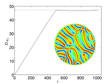
Figure 3: (color) The cumulative dimension of a flow field pattern where a single snapshot is rotated azimuthally by increments of $\Delta\theta=2\pi/512$ to form new snapshots where the angle of rotation is $\theta_{i}=i\Delta\theta$ and $i$ is an integer. Results are shown for a total of 1024 rotations where method of snapshots is the solid line and the Fourier method is the dashed line. The two methods agree when $i=512$ and $1024$ corresponding to one and two complete rotations of the flow field, respectively. The flow field used is at time $t=500$ (see inset) and for the simulation parameters $\Gamma=10$, $\sigma=1$, and $R/R_{c}=3.5$.

3 Discussion

3.1 Comparison of the method of snapshots and the Fourier method

We now illustrate the differences between the two methods through two examples using numerical data from our simulations for $\Gamma=10$. The flow field patterns from four instances in time separated by $50\tau_{v}$ are shown in Fig. 2. Using the Fourier method the dimensions of these individual images are $D_{KL}=46.1,46.8,49.8,48.5$ for panels (a)-(d), respectively. We next construct a time series out of these images and compute the dimension using images from panels (a), (a,b), (a,b,c), and (a,b,c,d) which we refer to as the cumulative dimension in Table 1. The magnitude of the dimension increases rapidly with the addition of each new flow field image. When using all four images the Fourier method yields a dimension of $D_{KL}=147.4$ which is less than the sum of the individual contributions 191.2.

The method of snapshots, which does not take advantage of the rotational invariance of the flow field, has only a dimension of 3.49 when using all four images. This comparison illustrates the rapid convergence of the Fourier method for the computation of $D_{KL}$ in high-dimensional systems.

Using the same convection domain with $\Gamma=10$ we now consider a single flow field image from time $t=500$ that is rotated azimuthally in small increments to create a series of images that is then used to compute $D_{KL}$. The specific flow field pattern that is used is shown in the inset of Fig. 3. The image is rotated incrementally by $\Delta\theta=2\pi/512$ to yield rotations of $\theta=i\Delta\theta$ where $i=1,2,\ldots,1024$ resulting in two complete rotations.

The values of $D_{KL}$ from the method of snapshots and the Fourier method are shown in Fig. 3. The dimension from the Fourier method is $D_{KL}=47.3$ using only one image and remains at this value for the subsequent incremental rotations. The method of snapshots however, increases monotonically for each incremental rotation and agrees with the dimension from the Fourier method only after one complete rotation. This occurs for subsequent complete rotations as well.

This example illustrates the clear computational advantage, in terms of rate of convergence, of the Fourier method for computing $D_{KL}$. It also shows that both the method of snapshots and the Fourier method eventually yield the same value for $D_{KL}$. The computed values of $D_{KL}$ only agree after the flow field pattern has undergone a complete rotation. For the case of actual flow field data it is expected that the two approaches would also agree if enough data were used for the method of snapshots to sample from all of the possible orientations. However, this can be a very slow process as we will demonstrate.

3.2 The Lyapunov and Karhunen-Loève dimensions

A significant advantage of studying chaotic Rayleigh-Bénard convection is that the spectrum of Lyapunov exponents have been calculated to yield quantitative measurements of the Lyapunov dimension [18, 19]. The spectrum of Lyapunov exponents $\lambda_{j}$ measure the exponential separation of trajectories in phase space and are ordered from largest to smallest. A single positive exponent is the defining feature of deterministic chaos (c.f. [1, 30, 31]). The sum of the first $N$ exponents indicates the exponential growth of an $N-$dimensional ball of initial conditions in phase space. The number of exponents that must be added in order for their sum to equal zero yields the Lyapunov dimension. Using a linear interpolation to find the precise value of this number is the commonly used Kaplan-Yorke formula [32],

$$D_{\lambda}=J+\frac{S_{J}}{|\lambda_{J+1}|}$$ (19)

where $J$ is the largest $j$ for which

$$S_{J}=\sum_{j=1}^{J}\lambda_{j}>0.$$ (20)

The Lyapunov dimension $D_{\lambda}$ is an approximation to the number of degrees of freedom that contribute to the chaotic dynamics [33, 1].

The Karhunen-Loève dimension was compared with the Lyapunov dimension by Sirovich and Deane [34] as the Rayleigh number was varied for turbulent Rayleigh-Bénard convection in a small periodic domain with free surface boundary conditions. Zoldi et al. [35] computed $D_{KL}$ from experimental shadowgraph images of the spiral defect chaos state [36] of Rayleigh-Bénard convection in a large cylindrical domain with $\Gamma=109$. In order to explore the variation of $D_{KL}$ with the system size the data was spatially sampled with a window of increasing size. Using this approach it was found that $D_{KL}$ scaled linearly with window size demonstrating extensivity. For Rayleigh-Bénard convection in a shallow layer there are effectively two spatially extended directions and, as a result, the system size is measured as $\Gamma^{2}$.

The spiral defect chaos state has also been explored numerically. Using a range of large periodic box geometries $D_{\lambda}$ was found to scale extensively with system size for $\Gamma=48,56,64$ and $R/R_{c}=1.8$ [18]. For box geometries the aspect ratio is defined as $\Gamma=L/d$ where $L$ is the length of an entire side of the box. The dimension $D_{\lambda}\approx 80$ for the largest domain and the dimension density was found to be $\delta_{\lambda}=D_{\lambda}/\Gamma^{2}\approx 0.019$. The extensivity of chaos was also shown numerically for a range of finite cylindrical geometries for $4.72\leq\Gamma\leq 15$, $\sigma=1$, and $R/R_{c}=3.5$ [19]. In this case the dimension density was found to be $\delta_{\lambda}\approx 0.25$. In our study we have chosen to explore the same system parameters as those of Ref. [19] and to compute the variation of $D_{KL}$ over the same range of system sizes.

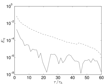
Figure 4: The convergence of the normalized eigenvalue spectrum as a function of time $\tau$ for $\Gamma=6$ where the time has been normalized by the horizontal diffusion time $\tau_{h}$. The error is given by $E_{\eta}$ for the method of snapshots (dashed line) and the Fourier method (solid line).

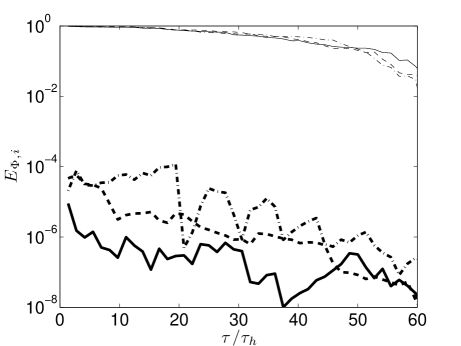
Figure 5: The convergence of the eigenfunctions with time for a convection domain with aspect ratio $\Gamma=6$. The error in the eigenfunction for mode $i$ is given by $E_{\Phi,i}$. Results are shown for $i=1$ (solid lines), $i=25$ (dashed lines), and $i=50$ (dash-dotted lines). The results computed using the method of snapshots are represented by thin lines and those using the Fourier method are represented by thick lines.

3.3 Convergence of the eigenvalues and eigenfunctions

We next examine the convergence of the normalized eigenvalue distribution

$$\eta_{i}=\frac{\mu_{i}}{\displaystyle\sum_{i}\mu_{i}},$$ (21)

where the index $i$ is over all computed eigenvalues $\mu_{i}$. The variation of magnitude of the error with time $E_{\eta}(\tau)$ is computed as,

$$E_{\eta}(\tau)=1-\frac{|\eta_{i}(\tau)|}{|\eta_{i,\infty}|}$$ (22)

where $|\eta_{i}|$ is the magnitude of the eigenvalue spectrum and $|\eta_{i,\infty}|$ is the value using the largest $\tau$ available for each case. The error $E_{\eta}$ decreases rapidly with time and is shown in Fig. 4. The time has been normalized by the nondimensional time required for heat to diffuse a distance $r_{0}$ which we refer to as the horizontal diffusion time $\tau_{h}=\Gamma^{2}$. The nondimensional time scale of the fluid motion in a convection roll is on the order of $\tau\approx 1$ and $\tau_{h}$ represents a long-time scale. The convergence rate of the Fourier method is again found to be faster than the method of snapshots. For $\tau\approx 5\tau_{h}$ the error is $E_{\eta}\sim 10^{-2}$ using the method of snapshots and $E_{\eta}\sim 10^{-4}$ using the Fourier method.

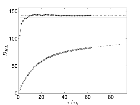
Figure 6: The variation of $D_{KL}$ with time for the Fourier method ($\star$) and the method of snapshots ($\circ$) for $\Gamma=6$. The converged value for the Fourier method is given by the dash-dotted line. The curve fit for the method of snapshots is $D_{KL}=137.8-68.4\exp{(-0.0730\tau/\tau_{h})}-69.3\exp{(-0.00406\tau/\tau_{h})}$ and is given by the dashed line. The asymptotic value of the dimension for the method of snapshots is given by the solid line at $D_{\infty}=137.8$.

The convergence of the POD modes depend upon their eigenvalue and Fig. 5 shows the convergence of modes 1, 25, and 50. Again we use the data for the largest available $\tau$ as an approximation for $\tau\rightarrow\infty$. The time variation of the magnitude of the error for the $i$th mode is computed as

$$E_{\Phi,i}(\tau)=1-\frac{(\bm{\Phi}_{i}(\tau),\bm{\Phi}_{i,\infty})}{(\bm{\Phi}_{i,\infty},\bm{\Phi}_{i,\infty})}.$$ (23)

Again, the Fourier method converges faster than the method of snapshots.

3.4 The convergence of the Karhunen-Loève dimension

The convergence of $D_{KL}$ for $\Gamma=6$ with respect to time is shown in Fig. 6. where the time has been scaled by the horizontal diffusion time $\tau_{h}$. Results are given for both the Fourier method and the method of snapshots. The Fourier method has reached a value of $D_{KL}\approx 142$ after $\tau\approx 20\tau_{h}$.

On the other hand, the method of snapshots exhibits a very gradual convergence. The numerical simulations were continued until $\tau\approx 60\tau_{h}$. In order to estimate a value of the asymptotic value of the dimension $D_{\infty}$ for the method of snapshots the results are fit with the following exponential dependence,

$$D_{KL}(\tau)=D_{\infty}+c_{1}\exp{(-c_{2}\frac{\tau}{\tau_{h}})}+c_{3}\exp{(-c_{4}\frac{\tau}{\tau_{h}})}$$ (24)

which is shown as the dashed line. The fitted curve is used to determine the asymptotic value of the dimension to yield $D_{\infty}=137.8$ and is indicated by the solid line. The convergence is very slow. For the dimension to converge within 10% of $D_{\infty}$ requires a time of $\tau\sim 400\tau_{h}$. Such a slow convergence rate in time is typical of our results for the method of snapshots. A further difficulty resulting from the slow convergence is the that the value of $D_{\infty}$ is very sensitive to small variations in the data that is made more significant when only a finite amount of data is available. The variation of $D_{KL}$ with time is shown for $\Gamma=10,12,15$ in Figs. 7-9 respectively and numerical values of the $D_{KL}$ are given in Table 2.

Table 2: The variation of the dimension with system size. The asymptotic values of the Karhunen-Loève dimension $D_{\infty}$ are given for the method of snapshots and the Fourier method. The Lyapunov dimension $D_{\lambda}$ computed for the same system parameters are included from Ref. [19].

	Snapshots	Fourier Method	Lyapunov
$\Gamma$	$D_{KL}$	$D_{KL}$	$D_{\lambda}$
6	138	142	6.8
10	265	409	21.6
12	632	570	32.5
15	1320	1045	53.7

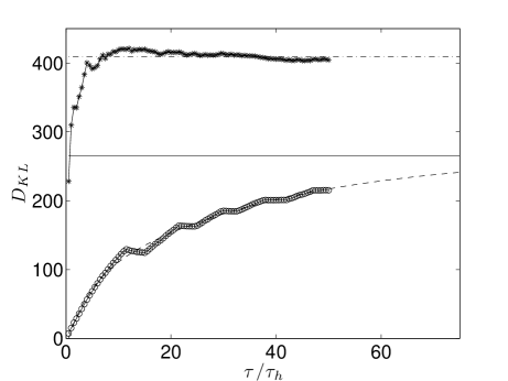
Figure 7: The variation of $D_{KL}$ with time $\tau$ for the Fourier method ($\star$) and the method of snapshots ($\circ$) for $\Gamma=10$. The converged value for the Fourier method is given by the dash-dotted line. The curve fit for the method of snapshots is $D_{KL}(\tau)=265.2-82.0\exp{(-0.2455\tau/\tau_{h})}-194.8\exp{(-0.02796\tau/\tau_{h})}$ and is given by the dashed line. The asymptotic value of the dimension for the method of snapshots is given by the solid line at $D_{\infty}=265.2$.

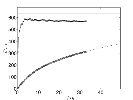
Figure 8: The variation of $D_{KL}$ with time $\tau$ for the Fourier method ($\star$) and the method of snapshots ($\circ$) for $\Gamma=12$. The converged value for the Fourier method is given by the dash-dotted line. The curve fit for the method of snapshots is $D_{KL}(\tau)=632.2-130.6\exp{(-0.1444\tau/\tau_{h})}-504.2\exp{(-0.01404\tau/\tau_{h})}$ and is given by the dashed line. The asymptotic value of the dimension for the method of snapshots is given by the solid line at $D_{\infty}=632.2$.

3.5 Extensivity

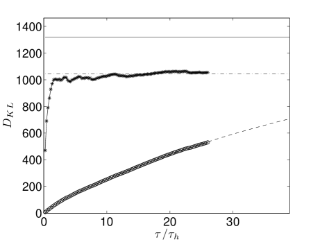
Figure 9: The variation of $D_{KL}$ with time $\tau$ for the Fourier method ($\star$) and the method of snapshots ($\circ$) for $\Gamma=15$. The converged value for the Fourier method is given by the dash-dotted line. The curve fit for the method of snapshots is $D_{KL}(\tau)=1320.1-36.5\exp{(-0.7892\tau/\tau_{h})}-1290.3\exp{(-0.01908\tau/\tau_{h})}$ and is given by the dashed line. The asymptotic value of the dimension for the method of snapshots is given by the solid line at $D_{\infty}=1320.1$.

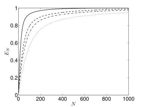
Figure 10: The fraction of the total energy captured $E_{N}$ as a function of the number of modes $N$ using the Fourier method. Results are shown for $\Gamma=6$ (solid line), $\Gamma=10$ (dashed line), $\Gamma=12$ (dash-dotted line), and $\Gamma=15$ (dotted line). A typical approach used to compute the value of $D_{KL}$ is to use the number of modes needed for $E_{N}=0.9$. From these results it is clear that $D_{KL}$ increases in value as the system size is increased.

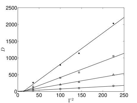
Figure 11: The variation of the dimension $D_{KL}$ with system size $\Gamma^{2}$ for several choices of $f$ using the Fourier method. Results are shown for $f=0.5$ (circles), $f=0.8$ (triangles), $f=0.9$ (squares), and $f=0.95$ (stars). The solid lines are linear curve fits through the data indicating the extensivity of $D_{KL}$. In the following figures we have chosen to use $f=0.9$ when reporting values of $D_{KL}$.

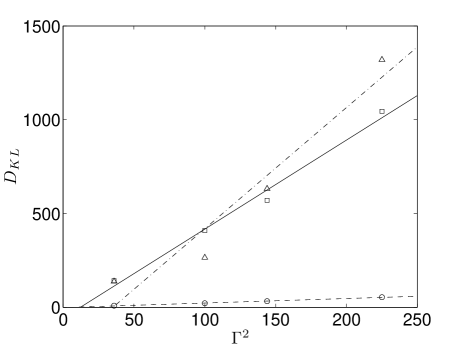
Figure 12: The variation of $D_{KL}$ and $D_{\lambda}$ with system size $\Gamma^{2}$ using numerical results for $\Gamma=6,10,12$ and $15$. The values of $D_{KL}$ computed using the Fourier method are represented as squares and the solid line is a linear curve fit. The value of $D_{KL}$ computed using the method of snapshots are represented as triangles and the dash-dot line is a linear curve fit. The Lyapunov dimension from Ref. [19] are represented as circles and the dashed line is a linear curve fit. From the data $D_{KL}\approx 19.7D_{\lambda}$ where the Fourier method has been used for $D_{KL}$.

Figure 10 shows the time variation of the cumulative normalized energy of the first $N$ eigenvalues. The normalized energy is computed from,

$$E_{N}(\tau)=\frac{\displaystyle\sum_{k=0}^{N}\mu_{k}}{\displaystyle\sum_{k=0}^{\infty}\mu_{k}}$$ (25)

using the data from the Fourier method with the largest $\tau$ for each respective system size. The basic trend of $E_{N}(\tau)$ shows that the total number of modes $N$ needed to capture a fraction $f$ increases with system size. Figure 11 shows the variation of $D_{KL}$ with system size using different values of $f$ where $0.5\leq f\leq 0.95$. Our results yield a linear relationship between $D_{KL}$ and $\Gamma^{2}$ over the entire range. The choice for $D_{KL}$ that we have used for reporting values of $D_{KL}$ is $f=0.9$.

The variation of $D_{KL}$ with system size is shown in Fig. 12 using the Fourier method (squares) and the method of snapshots (triangles) and linear curve fits through the data are given by the solid line and the dash-dotted line, respectively. The results using the method of snapshots increase with system size but with with significant deviations from the line of extensivity. As discussed, the rate of convergence for the method of snapshots is very slow and our numerical results would need to be continued for much longer simulation times for these results to converge. However, if this were done the results would eventually agree with those of the Fourier method which is extensive.

The variation of $D_{\lambda}$ with system size is shown in Fig. 12 by the circles with a linear curve fit given by the dashed line. Although there is no reason to expect the two dimensions to be related since they measure very different aspects of the patterns and their dynamics, it has been suggested that for extensively chaotic dynamics their rate of increase should be similar [37]. Numerical values of the dimensions are given in Table 2. Using the linear curve fits through the data yields the relationship $D_{KL}\approx 19.7D_{\lambda}$.

4 Conclusions

We have performed a proper orthogonal decomposition on a finite cylindrical domain containing a shallow fluid layer undergoing extensively chaotic dynamics. Our results suggest that even for this case the required time necessary to obtain good estimates of the Karhunen-Loève dimension are very long and on the order of hundreds of horizontal diffusion times with the commonly used method of snapshots. However, by exploiting the rotational symmetry of the problem the time to convergence can be drastically reduced using the Fourier method. This has important consequences for more complex flow fields that are common in engineering applications where the amount of data available is limited in both experiment and for computations. A prime example is the use of particle image velocimetry to obtained detailed information about the flow field. In this case the observation time is a function of the amount of data that can be captured by the camera. Overall, our results show that one must be careful to ensure the convergence of the proper orthogonal decomposition in order to obtain an accurate estimation of the dimension.

References

- [1] M. C. Cross, P. C. Hohenberg, Pattern formation outside of equilibrium, Rev. of Mod. Phys. 65 (3 II) (1993) 851–1112.
- [2] J. L. Lumley, The structure of inhomogeneous turbulent flows, Nauka, Moscow, 1967.
- [3] L. Sirovich, Turbulence and the dynamics of coherent structures. Part I: Coherent structures, Q. Appl. Math. XLV (3) (1987) 561–571.
- [4] L. Sirovich, Turbulence and the dynamics of coherent structures, Part II: Symmetries and transformations, Q. Appl. Math. XLV (3) (1987) 573–582.
- [5] L. Sirovich, Turbulence and the dynamics of coherent structures, Part III: Dynamics and scaling, Q. Appl. Math. XLV (3) (1987) 583–590.
- [6] L. Sirovich, Chaotic dynamics of coherent structures, Phys. D 37 (1989) 126.
- [7] L. Sirovich, K. S. Ball, L. R. Keefe, Plane waves and structures in turbulent channel flow, Phys. Fluids A 12 (1990) 2217–2226.
- [8] L. Sirovich, K. S. Ball, R. A. Handler, Propagating structures in wall-bounded turbulent flows, Theoret. Comput. Fluid Dynamics 2 (1991) 307.
- [9] K. S. Ball, L. Sirovich, L. R. Keefe, Dynamical eigenfunction decomposition of turbulent channel flow, Int. J. Num. Meth. Fluids 12 (1991) 587.
- [10] A. Duggleby, K. S. Ball, M. R. Paul, P. F. Fischer, Dynamical eigenfunction decomposition of turbulent pipe flow, J. of Turbulence 8 (43).
- [11] A. Duggleby, K. S. Ball, M. Schwaenen, Structure and dynamics of low reynolds number turbulent pipe flow, Phil. Trans. Roy. Soc. A 347 (2009) 473–488.
- [12] G. A. Webber, R. A. Handler, L. Sirovich, Energy dynamics in a turbulent channel flow using the Karhunen-Loève approach, Int. J. Numer. Meth. Fluids 40 (2002) 1381–1400.
- [13] X. Zhou, L. Sirovich, Coherence and chaos in a model of the turbulent boundary layer, Phys. Fluids A 4 (1994) 2955–2974.
- [14] K. D. Housiadas, A. N.Beris, R. A. Handler, Viscoelastic effects on higher order statistics and on coherent structures in turbulent channel flow, Phys. Fluids 17 (3).
- [15] A. Duggleby, K. S. Ball, M. R. Paul, The effect of spanwise wall oscillation on turbulent pipe flow structures resulting in drag reduction, Phys. Fluids 19 (125107).
- [16] Y. Lian, W. Shyy, D. Vileru, B. Zhang, Membrane wing aerodynamics for micro air vehicles, Prog. Aero. Sci. 39 (6–7) (2003) 425–465.
- [17] B. Epureanu, K. Hall, E. Dowell, Reduced-order models of unsteady viscous flows in turbomachinery using viscous-inviscid coupling, J. Fluids and Structures 15 (2) (2001) 255–273.
- [18] D. A. Egolf, I. V. Melnikov, W. Pesch, R. E. Ecke, Mechanisms of extensive spatiotemporal chaos in Rayleigh-Bénard convection, Nature 404 (2000) 733–736.
- [19] M. R. Paul, M. I. Einarsson, M. Cross, P. Fischer, Extensive chaos in Rayleigh-Bénard convection, Phys. Rev. E 75 (045203).
- [20] E. Bodenschatz, W. Pesch, G. Ahlers, Recent developments in Rayleigh-Bénard convection, Annu. Rev. Fluid Mech. 32 (2000) 709–778.
- [21] G. Ahlers, Low temperature studies of the Rayleigh-Bénard instability and turbulence, Phys. Rev. Lett. 33 (20) (1974) 1185–1188.
- [22] A. Libchaber, J. Maurer, Local probe in a Rayleih-Bénard experiment in liquid helium, J. Physique Lett. 39 (1978) 369–372.
- [23] A. Pocheau, Transition to turbulence of convective flows in a cylindrical container, J. Phys. France 49 (1988) 1127–1145.
- [24] M. R. Paul, M. C. Cross, P. F. Fischer, H. S. Greenside, Power-law behavior of power spectra in low prandtl number Rayleigh-Bénard convection, Phys. Rev. Lett. 87 (15) (2001) 154501.
- [25] P. Fischer, A. Patera, Parallel simulation of viscous incompressible flows, Annu. Rev. Fluid Mech. 26 (1994) 483–527.
- [26] P. F. Fischer, An overlapping Schwarz method for spectral element solution of the incompressible Navier-Stokes equations, J. Comp. Phys. 133 (1997) 84–101.
- [27] H. M. Tufo, P. F. Fischer, Terascale spectral element algorithms and implementations, in: Proc. of the ACM/IEEE SC99 Conf. on High Performance Networking and Computing, IEEE Computer Soc., 1999, gordon Bell Prize paper.
- [28] M. R. Paul, K.-H. Chiam, M. C. Cross, P. F. Fischer, H. S. Greenside, Pattern formation and dynamics in rayleigh-Bénard convection: numerical simulations of experimentally realistic geometries, Physica D 184 (2003) 114–126.
- [29] P. Holmes, J. L. Lumley, G. Berkooz, Turbulence, coherent structures, dynamical systems, and symmetry, Cambridge University Press, Cambridge, UK, 1996.
- [30] J. P. Eckmann, D. Ruelle, Ergodic theory of chaos and strange attractors, Rev. Mod. Phys. 57 (3) (1985) 617–656.
- [31] A. Wolf, J. Swift, H. L. Swinney, A. Vastano, Determining lyapunov exponents from a time series, Physica D 16 (1985) 285–317.
- [32] J. Kaplan, J. Yorke, Chaotic behavior in multi-dimensional difference equations, in: Functional Differential Equations and the Approximation of Fixed Points, Vol. 730 of Lecture Notes in Mathematics, Springer, 1979, p. 228.
- [33] J. D. Farmer, E. Ott, J. A. Yorke, The dimension of chaotic attractors, Physica 7D (1983) 153–180.
- [34] L. Sirovich, A. E. Deane, A computational study of Rayleigh-Bénard convection. Part 2. dimension considerations, J. Fluid Mech. 222 (1991) 251–265.
- [35] S. M. Zoldi, J. Liu, K. M. S. Bajaj, H. S. Greenside, G. Ahlers, Extensive scaling and nonuniformity of the Karhunen-Loè decomposition for the spiral-defect chaos state, Phys. Rev. E. 58 (6) (1998) R6903–R6906.
- [36] S. W. Morris, E. Bodenschatz, D. S. Cannell, G. Ahlers, Spiral defect chaos in large aspect ratio Rayleigh-Bénard convection, Phys. Rev. Lett. 71 (13) (1993) 2026–2029.
- [37] S. M. Zoldi, H. S. Greenside, Karhunen-Loève decomposition of extensive chaos, Phys. Rev. Lett. 78 (9) (1997) 1687–1690.