Analytical calculation of the excess current in the OTBK theory

Abstract

We present an analytical derivation of the excess current in Josephson junctions within the Octavio-Tinkham-Blonder-Klapwijk theory for both symmetric and asymmetric barrier strengths. We confirm the result found numerically by Flensberg et al. for equal barriers [Physical Review B 38, 8707 (1988)], including the prediction of negative excess current for low transparencies, and we generalize it for differing barriers. Our analytical formulae provide for convenient fitting of experimental data, also in the less studied, but practically relevant case of the barrier asymmetry.

1 Introduction

The transport in Josephson junctions with various different materials constituting the normal region has been a very active research field for decades now and continues to be one. Among the many interesting transport properties of Josephson junctions are the so-called subharmonic gap structure (SGS) and the excess current, both of which were accurately explained by the concept of multiple Andreev reflections (MAR). The MAR theory was first formulated for normal–superconducting (NS) interfaces by Blonder, Tinkham, and Klapwijk (BTK) [1, 2] and the BTK theory and its extensions (especially to the ferromagnetic or non-BCS superconducting contacts) are still actively used in fitting experiments [3, 4, 5] and in theoretical studies [6, 7].

The BTK theory was then extended to full SNS junctions by Octavio, Tinkham, Blonder and Klapwijk (OTBK) [8] and Flensberg, Bindslev Hansen and Octavio [9]. The OTKB approach does not keep track of the evolution of the quasiparticle phase between the interfaces and therefore assumes complete dephasing in the junction area. This assumption breaks down for sufficiently small systems such as, e.g., atomic wires and the fully coherent approach developed in mid 90’s [10, 11, 12] is applicable instead. Nevertheless, the OTBK theory describes certain systems, such as microbridges, very well and keeps on being used in the literature both in experimental [13, 14, 15, 16, 17, 18] as well as theoretical [19] studies. In particular, its extension to the experimentally relevant situation of asymmetric junctions was developed and applied in Refs. [13, 14, 15].

In this work we analytically study the excess current in the OTBK theory. Although the excess current has been derived analytically in more recent coherent theories [11] it has not been reported yet in an analytic form in the older incoherent OTBK approach. We fill in this gap and provide the analytical derivation of the excess current for incoherent generally asymmetric SNS junctions described by the OTBK theory. Our formula can be used for the experimental fitting but it also has implications for the understanding of the role of coherence within the junction as discussed in more detail in the concluding section.

2 OTBK model

$A(E)$	$B(E)$	$T(E)$
$\frac{\Delta^{2}}{E^{2}+(1+2Z^{2})^{2}(\Delta^{2}-E^{2})}$	$\frac{4Z^{2}(1+Z^{2})(\Delta^{2}-E^{2})}{E^{2}+(1+2Z^{2})^{2}(\Delta^{2}-E^{2})}$	0	for $\left|E\right|<\Delta$
$\frac{\Delta^{2}}{\left(E+(1+2Z^{2})\sqrt{E^{2}-\Delta^{2}}\right)^{2}}$	$\frac{4Z^{2}(1+Z^{2})(E^{2}-\Delta^{2})}{\left(E+(1+2Z^{2})\sqrt{E^{2}-\Delta^{2}}\right)^{2}}$	$\frac{2(E^{2}-\Delta^{2}+E(1+2Z^{2})\sqrt{E^{2}-\Delta^{2}})}{\left(E+(1+2Z^{2})\sqrt{E^{2}-\Delta^{2}}\right)^{2}}$	for $\left|E\right|>\Delta$

Table 1: The reflection and transmission probabilities for an NS-interface with the dimensionless barrier strength $Z$ (after Ref. [2]; modified).

The BTK theory describes the transport through a single normal–superconducting interface, which is assumed to consist of a ballistic superconductor in contact with an equally ballistic piece of normal metal. Scattering can thus only occur at the interface at $x=0$, which is modelled by a repulsive delta-function potential $H\delta(x),\,H\geq 0,$ with a dimensionless parameter $Z=H/\hbar v_{F}$ ($v_{\mathrm{F}}$ being the Fermi velocity) that represents the barrier strength [2]. Transport properties are found by matching the wave functions on either side of this barrier. The different allowed processes are identified and labelled as follows: Andreev reflection $A$, normal reflection $B$, and transmission $T$. The corresponding probabilities $A(E)$, $B(E)$ and $T(E)$ are expressed as functions of the quasiparticle energy $E$, the superconducting gap $\Delta$, and the interface’s barrier strength $Z$ (cf. Table 1). The electrons at the normal side of the interface are separated into left- and right-moving populations, represented by the distribution functions $f_{\leftarrow}(E)$ and $f_{\rightarrow}(E)$, respectively. The current through the interface is then given by

$$I=\frac{1}{eR_{0}}\int_{-\infty}^{\infty}dE\left(f_{\rightarrow}(E)-f_{\leftarrow}(E)\right),$$ (1)

where $R_{0}=\left(2N(0)e^{2}v_{\mathrm{F}}\mathcal{A}\right)^{-1}$ is the Sharvin resistance of the perfectly transparent interface ($Z=0$) with $\mathcal{A}$ being the effective cross section of the contact and $N(0)$ the (single spin) density of states at the Fermi energy $E_{\mathrm{F}}$. Blonder, Tinkham and Klapwijk showed [2] that the distribution function for the left-moving electrons is given by

$$f_{\leftarrow}(E)=A(E)\left[1-f_{\rightarrow}(-E)\right]+B(E)f_{\rightarrow}(E)+T(E)f_{0}(E),$$ (2)

with $f_{0}(E)$ being the thermal Fermi distribution function $f_{0}(E)=1/(1+\exp(\beta(E-\mu)))$, assuming that the incoming electrons are in thermal equilibrium with their respective leads at the temperature $1/k_{\mathrm{B}}\beta$ and the chemical potential $\mu$.

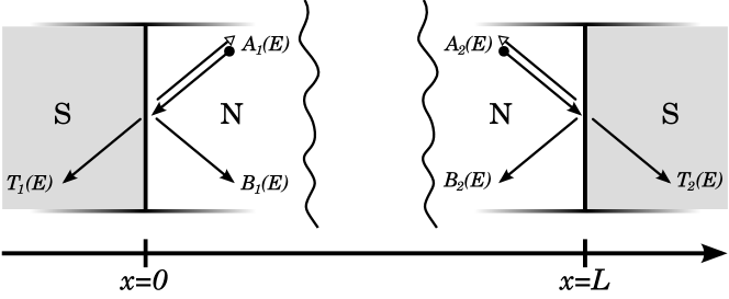
Figure 1: Schematic representation of an SNS junction, with arrows indicating the allowed processes at the interfaces: Andreev reflection $A$, normal reflection $B$ and transmission $T$.

This description was extended in Ref. [8] to an SN-interface followed by an NS-interface, i.e. to a full Josephson junction (cf. Figure 1). We assume the same superconducting material on both sides, i.e. the same superconducting gap $\Delta$, but different contacts and therefore differing barrier strenghts. We have interface $1$, located at $x=0$ with barrier strength $Z_{1}$, reflection and transmission probablities $A_{1}(E)$, $B_{1}(E)$ and, $T_{1}(E)$ and interface $2$, at $x=L$ with $Z_{2}$, $A_{2}(E)$, $B_{2}(E)$ and $T_{2}(E)$. The distribution functions $f_{\rightleftarrows}(E,x)$, which are again to be taken in the normal region, are also functions of the longitudinal position within the junction, $x$. Now Eq. (2) can be applied to each of the two interfaces, which yields the following two equations [8]

$$f_{\rightarrow}(E,0)=A_{1}(E)\left[1-f_{\leftarrow}(-E,0)\right]+B_{1}(E)f_{\leftarrow}(E,0)+T_{1}(E)f_{0}(E),$$ (3)

$$f_{\leftarrow}(E,L)=A_{2}(E)\left[1-f_{\rightarrow}(-E,L)\right]+B_{2}(E)f_{\rightarrow}(E,L)+T_{2}(E)f_{0}(E).$$ (4)

Note that we only combine distribution functions and not the quantum states (wavefunctions) at both interfaces. The relative phase of those states is therefore not considered, which is why the OTBK model only applies to incoherent junctions.

Since all energies are measured with respect to the local chemical potential, right-moving quasiparticles with energy $E$ at $x=0$ will arrive at $x=L$ with energy $E+eV$, while left movers with energy $E$ at $x=L$ will have energy $E-eV$ at $x=0$. Thus the distribution functions at the interfaces relate to each other as

$$f_{\rightleftarrows}(E,L)=f_{\rightleftarrows}(E-eV,0).$$ (5)

Eqs. (3)–(4) can be combined to eliminate, e.g., the left-moving part. Using Eq. (5) we can also shift all distribution functions from $x=L$ to $x=0$ and hence omit the position argument in the following. The following equation can then be derived [13]

$$f_{\rightarrow}(E) =A_{1}(E)\Bigl{\{}1-A_{2}(-E+eV)\bigl{[}1-f_{\rightarrow}(E-2eV)\bigr{]}$$

$$\qquad-B_{2}(-E+eV)f_{\rightarrow}(-E)-T_{2}(-E+eV)f_{0}(-E+eV)\Bigr{\}}$$

$$+B_{1}(E)\Bigl{\{}A_{2}(E+eV)\bigl{[}1-f_{\rightarrow}(-E-2eV)\bigr{]}$$

$$\qquad+B_{2}(E+eV)f_{\rightarrow}(E)+T_{2}(E+eV)f_{0}(E+eV)\Bigr{\}}$$

$$+T_{1}(E)f_{0}(E)$$

that couples $f_{\rightarrow}(E)$ with $f_{\rightarrow}(-E)$, $f_{\rightarrow}(E-2eV)$ and $f_{\rightarrow}(-E-2eV)$ and thus gives rise to an infinite system of linear equations for, say, $f_{\rightarrow}(E)$.

3 Equal barriers

The simplest case, as far as the barriers are concerned, is the the case in which both interfaces are characterized by the same barrier strength $Z_{1}=Z_{2}=Z$. For this case an additional relation $f_{\rightarrow}(E,0)=1-f_{\leftarrow}(-E,L)$ was derived in Ref. [9] from Eqs. (3)–(4) and substituted into Eq. (5), which yields

$$f_{\rightleftarrows}(E)=1-f_{\leftrightarrows}(-E-eV)$$ (7)

and greatly simplifies the problem. As before, the suppressed position arguments imply $x=0$. Using this result we can reformulate Eq. (1) to depend on right-movers only

$$I=\frac{1}{eR_{0}}\int_{-\infty}^{\infty}dE\left(f_{\rightarrow}(E)+f_{\rightarrow}(-E-eV)-1\right).$$ (8)

Furthermore we can make use of Eq. (7) to eliminate the distribution functions for left-moving electrons in Eq. (3), which yields a significantly simpler equation than the fully general one from OTBK (2), namely

$$f_{\rightarrow}(E)=A(E)f_{\rightarrow}(E-eV)+B(E)\left[1-f_{\rightarrow}(-E-eV)\right]+T(E)f_{0}(E).$$ (9)

The infinite system of linear equations generated by Eq. (9) was solved numerically in Ref. [9] to obtain subharmonic gap structure and excess current, but the latter can be obtained analytically [20], as we reproduce for convenience of the reader in the following.

3.1 Normal current

We shall first calculate the normal current to demonstrate the course of the derivation and to define some of the quantities used later on. We introduce the reflection and transmission probabilities in the normal case

$$B_{\mathrm{n}}=\frac{Z^{2}}{1+Z^{2}},\qquad T_{\mathrm{n}}=1-B_{\mathrm{n}}=\frac{1}{1+Z^{2}},$$ (10)

which are indeed the limits of $B(E)$ and $T(E)$ for vanishing $\Delta$, as can be seen from Table 1. This allows us to rewrite Eq. (9) for the normal case as

$$f_{\rightarrow}^{\mathrm{n}}(E)=B_{\mathrm{n}}\left[1-f_{\rightarrow}^{\mathrm{n}}(-E-eV)\right]+T_{\mathrm{n}}f_{0}(E),$$ (11)

where $f_{\rightarrow}^{\mathrm{n}}(E)$ is the right-moving distribution function for the normal case. We rewrite the above Eq. (11) for the energy $-E-eV$

$$f_{\rightarrow}^{\mathrm{n}}(-E-eV)=B_{\mathrm{n}}\left[1-f_{\rightarrow}^{\mathrm{n}}(E)\right]+T_{\mathrm{n}}f_{0}(-E-eV),$$ (12)

insert this again in Eq. (11) and solve for $f_{\rightarrow}^{\mathrm{n}}(E)$, which yields

$$f_{\rightarrow}^{\mathrm{n}}(E) =\frac{T_{\mathrm{n}}}{1-B_{\mathrm{n}}^{2}}f_{0}(E)+\frac{B_{\mathrm{n}}T_{\mathrm{n}}}{1-B_{\mathrm{n}}^{2}}f_{0}(E+eV)$$ (13)

$$=\frac{1+Z^{2}}{1+2Z^{2}}f_{0}(E)+\frac{Z^{2}}{1+2Z^{2}}f_{0}(E+eV),$$

where we have used that $f_{0}(-E-eV)=1-f_{0}(E+eV)$. We can write down the integrand from Eq. (8) with these normal-case distribution functions and simplify it to give

$$f_{\rightarrow}^{\mathrm{n}}(E)+f_{\rightarrow}^{\mathrm{n}}(-E-eV)-1=\frac{1+Z^{2}}{1+2Z^{2}}\bigl{(}f_{0}(E)+\overbrace{f_{0}(-E-eV)-1}^{-f_{0}(E+eV)}\bigr{)}$$

$$\qquad+\frac{Z^{2}}{1+2Z^{2}}\bigl{(}f_{0}(E+eV)+\underbrace{f_{0}(-E)-1}_{-f_{0}(-E)}\bigr{)}$$ (14)

$$=\bigl{(}f_{0}(E)-f_{0}(E+eV)\bigr{)}/(1+2Z^{2}),$$

which is easily integrated and yields the familiar result $I_{\mathrm{n}}=V/R_{\mathrm{n}}$, with the normal state resistance $R_{\mathrm{n}}=(1+2Z^{2})R_{0}$ of the two-interface ballistic sandwich.

3.2 Excess current

In the superconducting case we are interested in the excess current $I_{\mathrm{exc}}$ defined as $I_{\mathrm{exc}}=I-I_{\mathrm{n}}$ in the limit $eV\rightarrow\infty$, which is what we will assume in the rest of this section. We define $\Delta f_{\rightarrow}(E)=f_{\rightarrow}(E)-f_{\rightarrow}^{\mathrm{n}}(E)$, insert this into Eq. (8) and substract the normal part thus arriving at the formula for the excess current

$$I_{\mathrm{exc}}=\frac{1}{eR_{0}}\int_{-\infty}^{\infty}dE\ \big{(}\Delta f(E)+\Delta f(-E-eV)\big{)},$$ (15)

where we have dropped the arrows from the notation, as we are only dealing with right-movers in this section. To calculate $\Delta f(E)$ we define, similarly to the above, $\Delta B(E)=B(E)-B_{\mathrm{n}}$ and $\Delta T(E)=T(E)-T_{\mathrm{n}}$, substitute all these definitions into Eq. (9), and solve for $\Delta f(E)$ to obtain

$$\Delta f(E)= A(E)\bigl{[}f_{\mathrm{n}}(E-eV)+\Delta f(E-eV)\bigr{]}$$

$$+\Delta B(E)\bigl{[}1-f_{\mathrm{n}}(-E-eV)-\Delta f(-E-eV)\bigr{]}$$

$$-B_{\mathrm{n}}\Delta f(-E-eV)+\Delta T(E)f_{0}(E).$$

Examining Eq. (3.2) and keeping in mind that $A(E)$, $\Delta B(E)$ and $\Delta T(E)$ tend toward zero for $|E|\gg\Delta$, we see that there exists only a certain energy range $\epsilon$ of the order of a few multiples of $\Delta$ where $A(E)$, $\Delta B(E)$, and $\Delta T(E)$ can be considered non-zero such that $f(E)$ will only differ significantly from $f_{\mathrm{n}}(E)$ within $\epsilon$ around $E=0$ and $E=-eV$. Since we only consider large bias those two energy regions are well separated. Therefore we can split $\Delta f(E)$ into one part which is only nonzero for $|E|<\epsilon$ and vanishes for all other energies and one part with the same properties for $|E+eV|<\epsilon$. We introduce these parts by writing

$$\Delta f(E)=\Delta\tilde{f}(E)+\Delta\tilde{f}^{-eV}(E).$$ (17)

This mathematical procedure is fully in line with the physical intuition that the only changes of the distribution functions induced by the superconductivity will occur within the few-$\Delta$-multiples vicinity of the two Fermi energies of the leads. We can rewrite Eq. (3.2) for $\Delta f(E-eV)$ and we see that for $|E|<\epsilon$ most terms in the right hand side simply drop out as they include a vanishing multiplier. So we are left with

$$\Delta\tilde{f}^{-eV}(E-eV)=-B_{\mathrm{n}}\Delta\tilde{f}(-E).$$ (18)

We insert Eq. (18) into Eq. (3.2), still assuming $|E|<\epsilon$, to obtain

$$\Delta\tilde{f}(E)= A(E)\bigl{[}f_{\mathrm{n}}(E-eV)-B_{\mathrm{n}}\Delta\tilde{f}(-E)\bigr{]}$$

$$+\Delta B(E)\bigl{[}1-f_{\mathrm{n}}(-E-eV)+B_{\mathrm{n}}\Delta\tilde{f}(E)\bigr{]}$$

$$+B_{\mathrm{n}}^{2}\Delta\tilde{f}(E)+\Delta T(E)f_{0}(E).$$

It turns out to be convenient to consider the combination $\Delta\tilde{f}(E)+\Delta\tilde{f}(-E)$ in the following, i.e. to symmetrize the problem. Therefore, we rewrite Eq. (3.2) for $\Delta\tilde{f}(-E)$, sum the result with Eq. (3.2) and solve for $\Delta\tilde{f}(E)+\Delta\tilde{f}(-E)$ obtaining

$$\Bigl{[}1+B_{\mathrm{n}}\bigl{(}A(E)-B(E)\bigr{)}\Bigr{]}\Bigl{(}\Delta\tilde{f}(E)+\Delta\tilde{f}(-E)\Bigr{)}=$$

$$\!\!\!\!\!\!\!\!\!\!\!\!\!\!\!\!\!\!\bigl{(}A(E)-\Delta B(E)\bigr{)}\bigl{[}f_{\mathrm{n}}(E-eV)+f_{\mathrm{n}}(-E-eV)\bigr{]}+2\Delta B(E)+\Delta T(E).$$ (20)

Obviously, the above Eq. (20) again holds only for the range $|E|<\epsilon$ in which it was derived. The sum $f_{\mathrm{n}}(E-eV)+f_{\mathrm{n}}(-E-eV)$ that turns up on the right-hand side of Eq. (20) can be calculated using Eq. (13) and the assumption of large bias, i.e. $eV\rightarrow\infty$, so that we obtain

$$f_{\mathrm{n}}(E-eV)+f_{\mathrm{n}}(-E-eV) =\frac{1+Z^{2}}{1+2Z^{2}}\overbrace{\left(f_{0}(E-eV)+f_{0}(-E-eV)\right)}^{\longrightarrow 2}$$ (21)

$$+\frac{Z^{2}}{1+2Z^{2}}\underbrace{\left(f_{0}(E)+f_{0}(-E)\right)}_{1}=\frac{2+3Z^{2}}{1+2Z^{2}}.$$

From the condition of probability conservation $A(E)+B(E)+T(E)=1$, we see that $\Delta T(E)=-A(E)-\Delta B(E)$. We substitute this into Eq. (20) along with Eq. (21) and are left with

$$\Delta\tilde{f}(E)+\Delta\tilde{f}(-E)=\frac{\bigl{(}A(E)-\Delta B(E)\bigr{)}(1+Z^{2})}{\Bigl{[}1+B_{\mathrm{n}}\bigl{(}A(E)-B(E)\bigr{)}\Bigr{]}(1+2Z^{2})}.$$ (22)

We now take the integrand from Eq. (15) and expand it by inserting Eq. (17) to get

$$\Delta f(E)+\Delta f(-E-eV)=\Delta\tilde{f}(E)+\Delta\tilde{f}^{-eV}(E)+\Delta\tilde{f}(-E-eV)+\Delta\tilde{f}^{-eV}(-E-eV).$$ (23)

The first and the last terms are nonzero around $E=0$ and we can use the straightforward modification of Eq. (18) for the simplification $\Delta\tilde{f}(E)+\Delta\tilde{f}^{-eV}(-E-eV)=(1-B_{\mathrm{n}})\Delta\tilde{f}(E)$. Analogously, the two middle terms in Eq. (23) are nonzero around $E=-eV$ and since they appear under the integral extending over the entire energy range and have strongly localized support their energy arguments can be shifted so that they are localized around $E=0$ as well. This eventually leads to the relations $\Delta\tilde{f}^{-eV}(E)+\Delta\tilde{f}(-E-eV)\Rightarrow\Delta\tilde{f}^{-eV}(E-eV)+\Delta\tilde{f}(-E)=(1-B_{\mathrm{n}})\Delta\tilde{f}(-E)$. Putting all the pieces together leaves us with

$$I_{\mathrm{exc}} =\frac{1}{eR_{0}}\int_{-\infty}^{\infty}dE\ (1-B_{\mathrm{n}})\left(\Delta\tilde{f}(E)+\Delta\tilde{f}(-E)\right)$$ (24)

$$=\frac{1}{eR_{0}(1+2Z^{2})}\int_{-\infty}^{\infty}dE\ \frac{A(E)-\Delta B(E)}{\left[1+B_{\mathrm{n}}\left(A(E)-B(E)\right)\right]},$$

where we used Eq. (22) to produce the final integrand. The analytical integration must be performed for $\left|E\right|\leq\Delta$ and $\left|E\right|\geq\Delta$, separately, because $A(E)$ and $B(E)$ take on different functional forms in these intervals. It can be evaluated using trigonometric or hyperbolic substitution for the subgap or overgap energies, respectively. Thus we find the excess current in the symmetric case is given by

$$\frac{eI_{\mathrm{exc}}R_{\mathrm{n}}}{\Delta}= 2(1+2Z^{2})\mathrm{tanh}^{-1}\left(2Z\sqrt{(1+Z^{2})/(1+6Z^{2}+4Z^{4})}\right)$$ (25)

$$\qquad\times\left(Z\sqrt{(1+Z^{2})(1+6Z^{2}+4Z^{4})}\right)^{-1}-\frac{4}{3}.$$

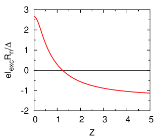
Figure 2: The excess current of a symmetric, fully incoherent Josephson junction in the OTBK model as a function of the barrier strength $Z$.

The first (and longer) term on the right hand side of Eq. (25) results from the subgap integral, the $-4/3$ term is the contribution of the overgap part. This analytic result is plotted in Figure 2 and the comparison with the earlier numerical result by Flensberg, Bindslev Hansen and Octavio plotted in Figure 6 of Ref. [9] shows a nice agreement.

4 Differing barrier strengths

To obtain a similar expression for the excess current in the case of asymmetric barrier strenghts we need to restart from Eq. (2), since Eq. (7) and the ensuing simplifications, in particular Eq. (9), cannot be used. The course of the derivation, however, is very similar to the above. Again we start by calculating the normal current.

4.1 Normal current

Corresponding to Eq. (1), the normal current is given by

$$I_{\mathrm{n}}=\frac{1}{eR_{0}}\int_{-\infty}^{\infty}dE\left(f_{\rightarrow}^{\mathrm{n}}(E)-f_{\leftarrow}^{\mathrm{n}}(E)\right),$$ (26)

where $f_{\rightarrow}^{\mathrm{n}}(E)$ is defined as above and $f_{\leftarrow}^{\mathrm{n}}(E)$ is its left-moving counterpart. The reflection and transmission probabilities in the normal case, $B_{\mathrm{n},i}$ and $T_{\mathrm{n},i}$, are defined as above with the additional index $i\in\{1;2\}$, which indicates the interface in question. From Eq. (2) we now find for the right-movers in the normal case

$$f_{\rightarrow}^{\mathrm{n}}(E)=B_{\mathrm{n},1}\left[B_{\mathrm{n},2}f_{\rightarrow}^{\mathrm{n}}(E)+T_{\mathrm{n},2}f_{0}(E+eV)\right]+T_{\mathrm{n},1}f_{0}(E).\\$$ (27)

Since we also need to consider left-movers in this section, we use Eqs. (3)–(5) to derive the left-moving counterpart to Eq. (2), which is not shown for reasons of length, and finally the equivalent of the above Eq. (27) for left movers, which reads

$$f_{\leftarrow}^{\mathrm{n}}(E)=B_{\mathrm{n},2}\left[B_{\mathrm{n},1}f_{\leftarrow}^{\mathrm{n}}(E)+T_{\mathrm{n},1}f_{0}(E)\right]+T_{\mathrm{n},2}f_{0}(E+eV).$$ (28)

We take the integrand from Eq. (26) and use Eqs. (27)–(28) to rewrite it as follows

$$f_{\rightarrow}^{\mathrm{n}}(E)-f_{\leftarrow}^{\mathrm{n}}(E) =\frac{T_{\mathrm{n},1}T_{\mathrm{n},2}}{1-B_{\mathrm{n},1}B_{\mathrm{n},2}}\left(f_{0}(E)-f_{0}(E+eV)\right)$$ (29)

$$=\frac{1}{1+Z_{1}^{2}+Z_{2}^{2}}\left(f_{0}(E)-f_{0}(E+eV)\right),$$

This is easy to integrate and yields $I_{\mathrm{n}}=V/(\rho_{\mathrm{n}}R_{0})$, with $\rho_{\mathrm{n}}=1+Z_{1}^{2}+Z_{2}^{2}$. Note that $\rho_{\mathrm{n}}R_{0}$ simply becomes $R_{\mathrm{n}}$ for $Z_{1}=Z_{2}=Z$, so we find the normal current from above for equal barriers again.

4.2 Excess current

For the calculation of the excess current we assume large bias once again and introduce $\Delta f_{\rightarrow}(E)=f_{\rightarrow}(E)-f_{\rightarrow}^{\mathrm{n}}(E)$, $\Delta B_{i}(E)=B_{i}(E)-B_{\mathrm{n},i}$ and $\Delta T_{i}(E)=T_{i}(E)-T_{\mathrm{n},i}$, just like above in the case of symmetric barriers. Using these relations we can expand Eq. (2) and subtract Eq. (27) to obtain

$$\Delta f_{\rightarrow}(E)= A_{1}(E)\Bigl{\{}1-A_{2}(-E+eV)\bigl{[}1-f_{\rightarrow}(E-2eV)\bigr{]}$$

$$\qquad-B_{2}(-E+eV)f_{\rightarrow}(-E)$$

$$\qquad-T_{2}(-E+eV)f_{0}(-E+eV)\Bigr{\}}$$

$$+B_{\mathrm{n},1}\Bigl{\{}A_{2}(E+eV)\bigl{[}1-f_{\rightarrow}(-E-2eV)\bigr{]}+B_{\mathrm{n},2}\Delta f_{\rightarrow}(E)$$

$$\qquad+\Delta B_{2}(E+eV)f_{\rightarrow}(E)+\Delta T_{2}(E+eV)f_{0}(E+eV)\Bigr{\}}$$

$$+\Delta B_{1}(E)\Bigl{\{}A_{2}(E+eV)\bigl{[}1-f_{\rightarrow}(-E-2eV)\bigr{]}$$

$$\qquad+B_{2}(E+eV)f_{\rightarrow}(E)+T_{2}(E+eV)f_{0}(E+eV)\Bigr{\}}$$

$$+\Delta T_{1}(E)f_{0}(E).$$

By the same logic as before we see that $\Delta f_{\rightarrow}(E)$ is only nonzero for $|E|<\epsilon$ or $|E+eV|<\epsilon$. Therefore we split $\Delta f_{\rightarrow}(E)$ into two parts, just like we did above and with the same properties

$$\Delta f_{\rightarrow}(E)=\Delta\tilde{f}_{\rightarrow}(E)+\Delta\tilde{f}_{\rightarrow}^{-eV}(E).$$ (31)

For the remainder of the section we assume small energies ($|E|<\epsilon$), in which case Eq. (4.2) can be reduced and solved for $\Delta\tilde{f}_{\rightarrow}(E)$ to yield

$$\bigl{[}1-B_{1}(E)B_{\mathrm{n},2}\bigr{]}\Delta\tilde{f}_{\rightarrow}(E) =A_{1}(E)\bigl{[}1-B_{\mathrm{n},2}\bigl{(}f_{\rightarrow}^{\mathrm{n}}(-E)+\Delta\tilde{f}_{\rightarrow}(-E)\bigr{)}$$

$$\qquad-T_{\mathrm{n},2}f_{0}(-E+eV)\bigr{]}$$

$$+\Delta B_{1}(E)\bigl{[}B_{\mathrm{n},2}f_{\rightarrow}^{\mathrm{n}}(E)+T_{\mathrm{n},2}f_{0}(E+eV)\bigr{]}$$

$$+\Delta T_{1}(E)f_{0}(E)$$

We rewrite Eq. (4.2) for $\Delta\tilde{f}_{\rightarrow}(-E)$, sum the result with Eq. (4.2) and solve for $\Delta\tilde{f}_{\rightarrow}(E)+\Delta\tilde{f}_{\rightarrow}(-E)$, which gives

$$\bigl{[}1+B_{\mathrm{n},2}\bigl{(}A_{1}(E)-B_{1}(E)\bigr{)}\bigr{]}\bigl{[}\Delta\tilde{f}_{\rightarrow}(E)+\Delta\tilde{f}_{\rightarrow}(-E)\bigr{]}$$

$$=A_{1}(E)\bigl{[}2-B_{\mathrm{n},2}\bigl{(}f_{\rightarrow}^{\mathrm{n}}(E)+f_{\rightarrow}^{\mathrm{n}}(-E)\bigr{)}$$

$$\qquad-T_{\mathrm{n},2}\bigl{(}f_{0}(E+eV)+f_{0}(-E+eV)\bigr{)}\bigr{]}$$

$$+\Delta B_{1}(E)\bigl{[}B_{\mathrm{n},2}\bigl{(}f_{\rightarrow}^{\mathrm{n}}(E)+f_{\rightarrow}^{\mathrm{n}}(-E)\bigr{)}$$ (33)

$$\qquad+T_{\mathrm{n},2}\bigl{(}f_{0}(E+eV)+f_{0}(-E+eV)\bigr{)}\bigr{]}$$

$$+\Delta T_{1}(E)\underbrace{\bigl{(}f_{0}(E)+f_{0}(-E)\bigr{)}}_{1}$$

The sum $f_{0}(E+eV)+f_{0}(-E+eV)$ in the above becomes zero for large bias, which means that the terms explicitly involving $T_{\mathrm{n},2}$ drop out of Eq. (33). Furthermore, using Eq. (27) we can write

$$f_{\rightarrow}^{\mathrm{n}}(E)+f_{\rightarrow}^{\mathrm{n}}(-E)=\bigl{[}B_{\mathrm{n},1}T_{\mathrm{n},2}\overbrace{\bigl{(}f_{0}(E+eV)+f_{0}(-E+eV)\bigr{)}}^{\rightarrow 0}$$

$$+T_{\mathrm{n},1}\underbrace{\bigl{(}f_{0}(E)+f_{0}(-E)\bigr{)}}_{1}\bigr{]}/(1-B_{\mathrm{n},1}B_{\mathrm{n},2})=\frac{T_{\mathrm{n},1}}{1-B_{\mathrm{n},1}B_{\mathrm{n},2}},$$ (34)

further simplifying Eq. (33), which can now be written as

$$\Delta\tilde{f}_{\rightarrow}(E)+\Delta\tilde{f}_{\rightarrow}(-E)=\frac{\rho_{1}}{\rho_{\mathrm{n}}}\frac{A_{1}(E)-\Delta B_{1}(E)}{1+B_{\mathrm{n},2}\bigl{(}A_{1}(E)-B_{1}(E)\bigr{)}},$$ (35)

where $\rho_{i}=1/T_{\mathrm{n},i}=1+Z_{i}^{2}$ is the dimensionless resistance of the single $i$-th interface in the normal state. In a similar way and using the same assumptions, i.e. $eV\rightarrow\infty$ and $|E|<\epsilon$, we can show that

$$\Delta\tilde{f}_{\rightarrow}^{-eV}(E-eV)+\Delta\tilde{f}_{\rightarrow}^{-eV}(-E-eV)=-\frac{\rho_{2}}{\rho_{\mathrm{n}}}\frac{A_{2}(E)-\Delta B_{2}(E)}{1+B_{\mathrm{n},1}\bigl{(}A_{2}(E)-B_{2}(E)\bigr{)}}B_{\mathrm{n},1}.$$ (36)

We still need to get the left-moving equivalents of Eqs. (35), (36), so first we derive the counterpart to Eq. (4.2) for the left-movers, which is not shown, because the derivation follows the earlier pattern and does not deliver new insights. Just like above we can split $\Delta f_{\leftarrow}(E)$ up into

$$\Delta f_{\leftarrow}(E)=\Delta\tilde{f}_{\leftarrow}(E)+\Delta\tilde{f}_{\leftarrow}^{-eV}(E).$$ (37)

As for the right-movers and in much the same way we can show that for $|E|<\epsilon$ and $eV\rightarrow\infty$

$$\Delta\tilde{f}_{\leftarrow}(E)+\Delta\tilde{f}_{\leftarrow}(-E)=\frac{\rho_{1}}{\rho_{\mathrm{n}}}\frac{A_{1}(E)-\Delta B_{1}(E)}{1+B_{\mathrm{n},2}\bigl{(}A_{1}(E)-B_{1}(E)\bigr{)}}B_{\mathrm{n},2}$$ (38)

as well as

$$\Delta\tilde{f}_{\leftarrow}^{-eV}(E-eV)+\Delta\tilde{f}_{\leftarrow}^{-eV}(-E-eV)=-\frac{\rho_{2}}{\rho_{\mathrm{n}}}\frac{A_{2}(E)-\Delta B_{2}(E)}{1+B_{\mathrm{n},1}\bigl{(}A_{2}(E)-B_{2}(E)\bigr{)}}.$$ (39)

The excess current is now given by

$$I_{\mathrm{exc}} =\frac{1}{eR_{0}}\int_{-\infty}^{\infty}dE \bigl{(}\Delta f_{\rightarrow}(E)-\Delta f_{\leftarrow}(E)\bigr{)}$$

$$=\frac{1}{2eR_{0}}\int_{-\infty}^{\infty}dE \Bigl{(}\overbrace{\Delta\tilde{f}_{\rightarrow}(E)+\Delta\tilde{f}_{\rightarrow}(-E)}^{(\ref{eq:Deltaftildesum01})}+\overbrace{\Delta\tilde{f}_{\rightarrow}^{-eV}(E)+\Delta\tilde{f}_{\rightarrow}^{-eV}(-E)}^{(\ref{eq:Deltaftildesum02})^{\prime}}$$

$$-\underbrace{\bigl{[}\Delta\tilde{f}_{\leftarrow}(E)+\Delta\tilde{f}_{\leftarrow}(-E)\bigr{]}}_{(\ref{eq:Deltaftildesum03})}-\underbrace{\bigl{[}\Delta\tilde{f}_{\leftarrow}^{-eV}(E)+\Delta\tilde{f}_{\leftarrow}^{-eV}(-E)\bigr{]}}_{(\ref{eq:Deltaftildesum04})^{\prime}}\Bigr{)}.$$

The braces and brackets in Eq. (4.2) indicate which terms in the expression correspond to which one of the above equations. The primed brackets are shifted in energy, which does not matter to the final result, since the integral extends over the entire energy range and the integrands have strongly localized support. Finally we can express the excess current as

$$I_{\mathrm{exc}}=\frac{1}{2eR_{0}}\int_{-\infty}^{\infty}dE\Biggl{\{}\frac{\rho_{1}}{\rho_{\mathrm{n}}}\frac{A_{1}(E)-\Delta B_{1}(E)}{1+B_{\mathrm{n},2}\bigl{(}A_{1}(E)-B_{1}(E)\bigr{)}}(1-B_{\mathrm{n},2})+\{1\leftrightarrow 2\}\Biggr{\}}.$$ (41)

The integral in Eq. (41) can be solved and the result for $Z_{1}>Z_{2}$ is given by

$$\frac{eI_{\mathrm{exc}}\rho_{\mathrm{n}}R_{0}}{\Delta} =2\rho_{\mathrm{n}}\mathrm{tanh}^{-1}\left(2Z_{1}\sqrt{\rho_{1}/\big{(}2Z_{2}^{2}+(1+2Z_{1}^{2})^{2}\big{)}}\right)$$

$$\qquad\times\left(Z_{1}\sqrt{\rho_{1}\big{(}2Z_{2}^{2}+(1+2Z_{1}^{2})^{2}\big{)}}\right)^{-1}$$

$$+\left[\mathrm{tan}^{-1}\sqrt{(Z_{1}^{2}-Z_{2}^{2})/\rho_{\mathrm{n}}}-\mathrm{tanh}^{-1}\sqrt{(Z_{1}^{2}-Z_{2}^{2})/\rho_{\mathrm{n}}}\right]$$

$$\qquad\times\frac{(1+2Z_{1}^{2})(1+2Z_{2}^{2})}{2\sqrt{\rho_{\mathrm{n}}}(Z_{1}^{2}-Z_{2}^{2})^{\frac{3}{2}}}-1.$$

For $Z_{1}<Z_{2}$ the excess current is obtained by exchanging $Z_{1}$ and $Z_{2}$ in Eq. (4.2) and the result is thus symmetric with respect to the interchange of the two interfaces. Again, the first term (the first line) on the right hand side of Eq. (4.2) corresponds to the sub-gap integral and it is easy to see how for $Z_{1}=Z_{2}=Z$ it becomes the corresponding term in Eq. (25). The remaining two terms (the second line), which result from the over-gap integral, converge towards $-4/3$ for $Z_{1}\rightarrow Z_{2}$, as we now show by the Taylor expansion of $\mathrm{tan}^{-1}(z)=z-\frac{1}{3}z^{3}+\frac{1}{5}z^{5}-\frac{1}{7}z^{7}+\ldots$ and $\mathrm{tanh}^{-1}(z)=z+\frac{1}{3}z^{3}+\frac{1}{5}z^{5}+\frac{1}{7}z^{7}+\ldots$ resulting in $\mathrm{tan}^{-1}(z)-\mathrm{tanh}^{-1}(z)=-\frac{2}{3}z^{3}+O(z^{7})$ so that the square bracket in the second line of Eq. (4.2) tends to $-\frac{2}{3}\bigl{(}(Z_{1}^{2}-Z_{2}^{2})/\rho_{\mathrm{n}}\bigr{)}^{\frac{3}{2}}$ for $Z_{1}\rightarrow Z_{2}$. Therefore the last two lines of Eq. (4.2) reduce to $-\frac{(1+2Z_{1}^{2})(1+2Z_{2}^{2})}{3\rho_{\mathrm{n}}^{2}}-1$, which simply becomes $-4/3$ for $Z_{1}=Z_{2}$ and we thus recover Eq. (25) in the symmetric case. The full result (4.2) is plotted in Figure 3 as a function of the two barrier strengths $Z_{1,2}$. The negative excess current predicted for large enough normal-state resistance persists for asymmetric junctions $Z_{1}\neq Z_{2}$ with arbitrarily large asymmetry although its magnitude decreases (also note the prefactor $\rho_{\mathrm{n}}$ customarily multiplying the plotted excess current) and, thus, its experimental observation may be impeded by the asymmetry of real junctions.

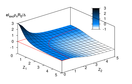
Figure 3: The excess current of an asymmetric, fully incoherent Josephson junction as a function of the two barrier strengths $Z_{1}$ and $Z_{2}$. The isoline $I_{\mathrm{exc}}=0$ is shown in red.

5 Conclusions and outlook

In this work we have analytically calculated the excess current within the OTBK theory describing fully incoherent SNS junctions. We have confirmed previous numerical findings [9] of negative excess current for large enough normal-state resistance in junctions with symmetric barriers. Furthermore, we extended those calculations also to the case of asymmetric barriers with qualitatively similar results, i.e. occurrence of negative excess current regardless of the asymmetry. Our formula (41) can be used also in the most general case of different superconducting leads, for an experiment see, e.g. Ref. [15], where $\Delta_{1}\neq\Delta_{2}$. The presence of two gap values prohibits further analytical treatment, however, Eq. (41) still holds and the integral can be easily evaluated numerically.

The numerical findings of Ref. [9] were challenged in Ref. [11] (p. 7372, paragraph below Eq. (30)) and the negativity of the excess current was interpreted as possibly stemming from a lack of convergence of the numerical study, i.e. from not reaching the true $eV\to\infty$ limit. Our study clearly demonstrates that this objection cannot hold since we explicitly work in the required limit, thus avoiding any finite-$V$ issues. We, however, do not question the presence of non-trivial issues in the experimental determination of the excess current related to the finite voltage and possible heating effects nicely reviewed and discussed in Ref. [12]. Apparently, observations of negative excess current (so called deficit current) have been reported in experiments [13, 14].

Nevertheless, we analytically prove the correctness of the old numerical results [9] predicting negative excess current within the OTBK theory. The discrepancy with the results of Ref. [11] then must stem from the difference of the two considered models, more specifically, the role of internal coherence of the junction. While the OTBK theory only considers matching of the distribution functions between the two interfaces corresponding to fully incoherent junctions, the Hamiltonian theory of Ref. [11] matches the wavefunctions throughout the whole junction thus fully retaining the coherence within the junction. The high-voltage properties of the two models differ even qualitatively, one predicting negative excess current for small transparencies, the other one not. Another qualitative difference between OTBK and the fully coherent theory is in their dependence on the junction asymmetry: While the fully coherent results in the limit of strong coherent coupling to the leads ($\Gamma_{1,2}\gg\Delta$, relevant for many experiments, e.g. [21, 22, 23]) only depend on the asymmetry through the total junction resistance [11], it is not so in the OTBK case as we can immediately see from our result for the excess current (Eq. (4.2)) which is not a function of $Z_{1}^{2}+Z_{2}^{2}$ only.

This finding shows that the coherence within the junction plays a crucial role for the superconducting transport even at finite voltage bias and therefore the level of decoherence/dephasing within a junction should be carefully considered when describing a particular experiment. This effect, i.e. nonzero dephasing within the junction, may be responsible for the experimentally observed discrepancies between the experiments [21, 22, 23] and theoretical predictions [11] systematically reported recently in Josephson junctions made of carbon nanotubes. While those discrepancies are currently interpreted as the superconducting gap renormalization this picture does not seem to be fully consistent with the positions of the subharmonic gap structure features, which appear at the positions determined by the un-renormalized gap value. The dephasing picture could capture the relevant physical mechanism instead although this remains an open issue in the currently booming field of superconducting transport in carbon-allotropes-based Josephson junctions.

Apart from the obvious usage of our newly derived analytical formulae for the OTBK excess current to fit experiments for relatively large and thus fully incoherent junctions, they can also be used as a limit benchmark of future partially-coherent theories, possibly relevant for current nanoscale experiments. These experiments as well as future devices built from novel low dimensional materials with peculiar electronic structures, such as graphene nanoribbons, could realistically be described by existing dephasing approaches for atomistic models [24, 25] coupled to non-equilibrium transport. The development of such a partially-coherent theory and the analytical evaluation of its excess current interpolating between the two limits is our next step.

References

References

- [1] Klapwijk T M, Blonder G E and Tinkham M 1982 Physica B+C 109-110 1657
- [2] Blonder G E, Tinkham M and Klapwijk T M 1982 Physical Review B 25 4515
- [3] Giubileo F, Aprili M, Bobba F, Piano S, Scarfato A and Cucolo A M 2005 Physical Review B 72 174518
- [4] Valentine J M and Chien C L 2006 Journal of Applied Physics 99 08P902
- [5] Cong Ren, Trbovic J, Kallaher R L, Braden J G, Parker J S, von Molnár S and Xiong P 2007 Physical Review B 75 205208
- [6] Xia K, Kelly P J, Bauer G E W and Turek I 2002 Physical Review Letters 89 166603
- [7] Linder J and Sudbø A 2008 Physical Review B 77 064507
- [8] Octavio M, Tinkham M, Blonder G E and Klapwijk T M 1983 Physical Review B, 27 6739
- [9] Flensberg K, Bindslev Hansen J and Octavio M 1988 Physical Review B 38 8707
- [10] Bratus’ E N, Shumeiko V S and Wendin G 1995 Physical Review Letters 74 2110
- [11] Cuevas J C, Martín-Rodero A and Levy Yeyati A 1996 Physical Review B 54 7366
- [12] Cuevas J C 1999 PhD thesis Universidad Autónoma de Madrid
- [13] van Huffelen W M, Klapwijk T M, Heslinga D R, de Boer M J and van der Post N 1993 Physical Review B 47 5170
- [14] Kuhlmann M, Zimermann U, Dikin D, Abens S, Keck K and Dmitriev V M 1994 Zeitschrift für Physik B 96 13
- [15] Zimermann U, Abens S, Dikin D, Keck K and Dmitriev V M 1995 Zeitschrift für Physik B 97 59
- [16] Baturina T, Islamov D and Kvon Z 2002 JETP Letters 75 326
- [17] Ishida H, Okanoue K, Kawakami A, Zhen Wang and Hamasaki K 2005 IEEE Transactions on Applied Superconductivity 15 212
- [18] Ojeda-Aristizàbal C M, Ferrier M, Guéron S and Bouchiat H 2009 arXiv:0903.2963
- [19] Pilgram S and Samuelsson P 2005 Physical Review Letters 94 086806
-
[20]
Niebler G, Cuniberti G and Novotný T 2008 in WDS’08
Proceedings of Contributed Papers: Part III – Physics 124
http://www.mff.cuni.cz/veda/konference/wds/contents/pdf08/WDS08_321_f3_Niebler.pdf - [21] Jørgensen H I, Grove-Rasmussen K, Novotný T, Flensberg K and Lindelof P E 2006 Physical Review Letters 96 207003
- [22] Jørgensen H I, Grove-Rasmussen K, Flensberg K and Lindelof P E 2008 arXiv:0812.4175
- [23] Wu F, Danneau R, Queipo P, Kauppinen E, Tsuneta T and Hakonen P J 2009 Physical Review B 79 073404
- [24] Pastawski H M 1991 Physical Review B 44 6329
- [25] Seelig G, Büttiker M 2001 Physical Review B 64 245313