Chaotic motion at the emergence of the time averaged energy decay

Abstract

A system plus environment conservative model is used to characterize the nonlinear dynamics when the time averaged energy for the system particle starts to decay. The system particle dynamics is regular for low values of the $N$ environment oscillators and becomes chaotic in the interval $13\leq N\leq 15$, where the system time averaged energy starts to decay. To characterize the nonlinear motion we estimate the Lyapunov exponent (LE), determine the power spectrum and the Kaplan-Yorke dimension. For much larger values of $N$ the energy of the system particle is completely transferred to the environment and the corresponding LEs decrease. Numerical evidences show the connection between the variations of the amplitude of the particles energy time oscillation with the time averaged energy decay and trapped trajectories.

Accepted Physica D

, ,

1 Introduction

Small dissipation is inevitable in real systems. In the Langevin description [1, 2] the damping force, together with the fluctuating force per unit mass (Langevin force), are used to model dissipation and friction. The damping force (or friction) is given by the Stoke’s law $F_{s}=-\gamma v$ and $\gamma$ is the damping constant. These forces represent the effect of the collisions of the system particle with the bath particles and are related via the dissipation-fluctuation theorem [2]. In the Langevin description we deal with a one-dimensional differential equation with dissipation. For higher-dimensional systems the whole dynamics follows the properties of many coexisting attractors. The characterization of this dynamics is not simple since high-dimensional systems usually present all characteristics of complexity [3], which may arise in the interplay between small dissipation and a conservative dynamics [3, 4]. Even for low-dimensional systems, elliptic periodic orbits become small sinks when small dissipation is added and an infinite number of periodic attractors may coexist [5]. Therefore, a nonlinear analysis on the borderline between small dissipation and a conservative dynamics is of interest for the description of complex systems in the real world.

Another possibility to describe dissipation is to consider an open system interacting with its environment by collision processes. The whole problem (System $+$ Environment $+$ Interaction) is conservative but, due to energy exchange between system and environment, the system can be interpreted as an open system with dissipation. Such a microscopic theoretical model has been proposed to describe dissipation processes in quantum [6, 7, 8] and in classical systems [1, 8]. In the limit of an infinite number of environment constituents, it is possible, in some specific cases, to derive a Langevin equation from the microscopic model [1]. Different from these works, in this paper the environment is composed of a finite number $N$ of uncoupled harmonic oscillators. Changing $N$ we are able to study the interesting transition from low- to high-dimensional dynamical systems which simultaneously experiment dissipation. The microscopic dynamics in this transition is not simple and its relation to macroscopic statistical mechanics is even more complicated. Such transitions started to be studied in the context of the Fermi-Pasta-Ulam (FPU) model [9] in order to answer questions related to irreversible statistical mechanics and equipartition of energy. The FPU model is a one-dimensional chain of $(N-1)$ coupled moving mass points (See Ford [10] for a nice review). The main problem was to explain the non-equipartition of energy observed for high values of $N$. With the help of chaos theory it became clear later that the equipartition of energy can be achieved at the strong stochasticity threshold [11]. In the model considered here the finite $N$ harmonic oscillators are indirectly coupled via the system particle. It is therefore a different physical situation from the FPU model and from the chaotic two-dimensional systems used to model thermal baths [12]. Beside that, it has been shown recently [13] that for finite values of $N$ the environment induces a non-Markovian motion on the system particle, and consequently, non-exponential energy decays. Therefore, our reservoir induces a damping mechanism which, in the Langevin description, corresponds to a complicated memory kernel [1] which only recovers the usual Stokes friction $\gamma$ in the limit $N\rightarrow\infty$ and for high environment frequencies (for details see [13]). In fact, our friction is determined during the time evolution through the dynamical process. Further, our damping mechanism differs from the velocity dependent friction in the Gaussian thermostat, obtained the requiring energy conservation at any time, and from the more general damping mechanism proposed in the Nosé-Hoover thermostat [14]. The finite $N$ model considered here has been used to study environment effects on the transport of particles in ratchets [15] and the role of Levy walks on the mobility in ratchet potentials [16].

In this paper we focus on the nonlinear dynamics of the time series obtained for the system particle under the $N$ harmonic oscillators. The tools used in this analysis are the Lyapunov spectrum [17], phase space dynamics, power spectrum and the Kaplan-Yorke dimension. Our system is deterministic and we use the TISEAN [18] package to analyse the time series [19]. The paper is organized as follows. Section 2 presents the model and Section 3 discusses the values of $N$ where the time averaged system energy starts to decay. In Section 4 results for the nonlinear time series analysis for one initial condition are presented. Lyapunov exponents, power spectrum and the Kaplan-York dimension are discussed. Finally in Section 5 the conclusions of the paper are presented.

2 The Model

Let us consider the problem composed by a particle under the influence of an asymmetric potential (the system) interacting with $N$ independent harmonic oscillators (the environment). The dimensionless equations of motion are (see [16] for more details)

$$\ddot{X}+\frac{dV(X)}{dX}-\sum_{j}^{N}{\gamma_{j}x_{j}}+X\sum_{j}^{N}{\frac{\gamma_{j}^{2}}{\mu_{j}w^{2}_{j}}}=0\textit{,}$$ (1)

$$\ddot{x}_{j}+{w^{2}_{j}}x_{j}-\frac{\gamma_{j}}{\mu_{j}}X=0~{}\textit{,}$$ (2)

where $X$ and ${\vec{x}}$ are, respectively, system and oscillators $(x_{j},j=1,2,...,N)$ coordinates. The coupling parameter $\gamma_{j}$ is a measure of the strength of the bilinear coupling between the system and the $j$-oscillator. The dimensionless anharmonic potential (see Fig. 1) is defined in the interval $X=(-0.38,0.62)$ by

$$V(X)=C-\frac{1}{4\pi^{2}\delta}\left[\sin{2\pi(X-X_{0})}+\frac{1}{4}\sin{4\pi(X-X_{0})}\right]~{}\textit{.}$$

The constant $C$ is such that $V(0)=0$. The time and the oscillators frequencies $w_{j}$ are written in units of $w_{0}=1.0$, which is the frequency of the linear motion around the minimum of the potential and is determined from $w^{2}_{0}={4\pi^{2}V_{0}\delta}/{M}$, where $\delta=\sin{2\pi|X^{\prime}_{0}|}+\sin{4\pi|X^{\prime}_{0}|}$. The dimensionless equations of motion (1) and (2) are the equations analyzed in this work. We used fourth-order Runge-Kutta integrator [20] with fixed step $\Delta t=10^{-3}$.

Figure 1: Dimensionless anharmonic potential $V(X)$ for $-0.38\leq X\leq 0.62$.

Some words about the model are in order. Although we solve all $2N+2$ equations of motion, the main dynamics is observed by the system particle. Usually in such system-plus-environment models with a bilinear coupling, the coordinates of the environment can be eliminated in the limit $N\rightarrow\infty$ and the resulting equation of motion for the system particle is a kind of Langevin equation [1, 7]. To notice in such approach is the assumption of weak coupling between the system and environment, and the infinite number of oscillators of the environment which characterize a thermal bath which is not affected by the system dynamics. Since in this work we investigate numerically the full set of equations of motion (1) and (2), the energy exchange and energy decay can be analyzed explicitly by increasing, one by one, the values of $N$.

For all cases considered in this paper, dimensionless mass $\mu_{j}=0.1$ and $\gamma_{j}=0.01$ are used. At time $t=0$, the system and the environment are not considered to be in equilibrium. The interaction energy is assumed to be zero, the energy of the system is very close to the total energy $E_{S}\sim E_{T}=0.02$, and the oscillators energy is close to zero ($E_{O}\sim 0.0$). The energy in all figures is adimensional. The initial distribution of the oscillators position and velocity is uniform around zero. For high values of $N$ the distribution of the oscillators frequencies approaches a quadratic (Debye-type) distribution with a cutoff at $w_{\mbox{cut}}=2.1$. The lower limit of this distribution is $w=1.1$.

In this work we kept the total energy $E_{T}$ fixed instead of the energy density $\varepsilon=E_{T}/N$. The reason to do this is simple. Our goal is to analyze the nonlinear dynamics of the system particle when energy is transferred from the system to the environment when $N=1\rightarrow 4000$. If we hold $\varepsilon$ fixed, two limiting situations are obtained. In the first one (when $N\rightarrow 4000$) we must increase $E_{T}$ and the system particle is not initially inside the potential well of Fig. (1). In such situation the particle will need a long time to loose its energy (via collisions with the $N$ oscillators) until it “falls down” into the potential well. When this happens, the physical situation is almost identical to the case discussed in this paper, where the particle starts inside the potential well. In the other limit (when $N=1$) the energy $E_{T}$ must be reduced very much and no energy transfer can be observed. In fact, both analysis could be implemented, but for the purpose of the present paper it is more appropriate to keep the total energy fixed.

3 Emergence of the time averaged energy decay

The system particle exchanges energy with the $N$ environment oscillators. This energy, continuously transferred to the environment, can return back to the system particle after a time of the order of the Poincaré recurrence time [7]. In general, for lower values of $N\lesssim 15$, the recurrence times are not very large and the energy return can be observed in simulations. However, for higher values of $N$, the Poincaré recurrence times increase very much to be observable with finite integration times. In such cases we can say that the energy transferred to the environment will not return, within the integration times, to the system particle. This is shown in

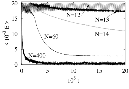
Figure 2: Mean energy (over $800$ environmental initial conditions) as a function of time for $N=12,13,14,60,400$.

Fig. 2, where the mean normalized system energy is plotted as a function of time for $N=12,13,14,60$ and $400$. For $N=12$ this energy oscillates strongly around the mean value $\sim 0.019$, but its time average is constant. For $N=13$ we see that, besides initial strong oscillations, the time averaged energy starts to decrease at times $t_{13}\sim 5\times 10^{3}$. This means that at times $t\sim t_{13}$ a portion of the system particle energy starts to be transferred to the environment without returning. For $N=14$ the time averaged energy starts to decay at times $t_{14}\sim 3\times 10^{3}$ and decreases continuously for the whole range of integration times. Increasing the values of $N$ to $60$ and $400$, we observe that the time at which the mean energy starts to be transferred to the environment gets smaller. It is interesting to observe that the particle energy starts to be transferred to the environment exactly when the amplitude of the large time oscillations of the mean energy decreases.

An interesting characteristic to mention from Fig. 2 is the non-exponential energy decay. For example, for $N=13$ the fit for the energy obeys $\left<E\right>\sim 0.029\ t^{-0.052}$ while for $N=400$ it obeys $\left<E\right>\sim 0.275\ t^{-0.733}$. Such power law behaviour is related to the non-Markovian dynamics induced by the environment and can be explained via environment autocorrelation function (see [13] for details.)

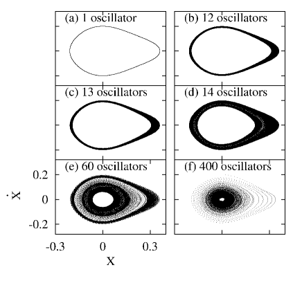
Figure 3: Phase space dynamics of the system particle for $N=1,12,13,14,60,400$.

Figure 3 shows the phase space dynamics of the system particle for $N=1,12,13,14,60,400$. For $N=1$ the dynamics is close to a deformed elliptic motion. As $N$ increases to $N=12,13,14$, the system particle exchanges energy with the oscillators and moves within a layer inside the deformed ellipsis. This layer increases as $N$ increases. For higher values of $N$ ($60$ and mainly $400$) the system particle rapidly loses its energy to the environment, and ends up moving close to the minimum of the anharmonic potential. When $N=4000$ (not shown) the system particle energy is close to zero and the energy per oscillator is also close to zero.

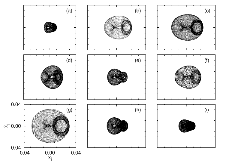
Figure 4: Phase space dynamics of the environment oscillators for $N=9$. From left to right and from top to bottom. The oscillators frequencies $w_{j}$ are (a) $2.089$, (b)$1.594$, (c) $1.529$, (d) $1.669$, (e) $1.875$, (f) $1.625$, (g) $1.414$, (h) $1.853$, (i) $1.969$.

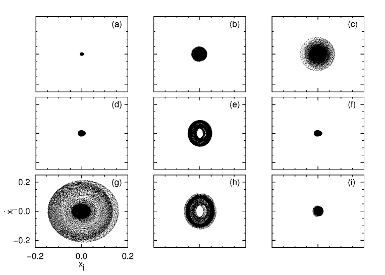
Figure 5: Phase space dynamics for the first nine environment oscillators for $N=15$. From left to right and from top to bottom. The frequencies are given in the caption of Fig. 4.

Figures 4 and 5 show respectively the phase space dynamics for the environment oscillators for $N=9$ and $N=15$. The oscillators are shown from left to right and from top to bottom. For $N=15$ we only display the first nine oscillators. For $N=9$ the shape of the curves in phase space are essentially governed by the frequency $w_{j}$ of each oscillator. The magnitudes of the oscillations in phase space (the size of the curves) are inversely proportional to the frequencies $w_{j}$. Environment oscillators with lower frequencies are more likely to receive the system particle energy and, consequently, the size of the oscillations increase. See for example the size of the lowest frequencies oscillations from Figs. 4(c) and (g). For oscillators with higher frequencies the size of the oscillations is smaller, as can be observed in Figs. 4(a) and (i). We essentially observe (together with conclusions obtained from Fig. 2) that for $N=9$ the system and oscillators just exchange energy continuously and the geometrical curves in phase space look “well behaved”. The shape of these curves does not change in time and consequently no equipartition of energy is observed for the integration times. For $N=15$ (see Fig. 5), when the time averaged energy decay has already occurred, all “well behaved” curves from the oscillators start to be destroyed and change in time. For small times (not shown) they look very similar to the curves from $N=9$, but for later times ($t>1.5\times 10^{3}$) they converge to the curves displayed in Fig. 5. Moreover, although energy is slowly shared between oscillators we observe that the magnitudes of oscillations in phase space are still different for distinct oscillators. For example, observe that the oscillation magnitude of case (g), with the lowest frequency, is much larger than the other ones (note that the scale from Fig. 5 differs from the scale of Fig. 4). This shows us again that we do not have equipartition of energy. We also determined the oscillator phase space dynamics for $N=4000$ (not shown) and non-equipartition of energy was observed.

Concluding this section we observe that the time averaged energy decay for the system particle starts to occur in the interval $N=(12,14)$. For lower values of $N$ the system continuously exchange energy with the environment but the time average is constant. For much higher values of $N$ the system particle energy is transferred to the environment for times very close to zero. The above mentioned interval $N=(12,14)$ is valid for the specific oscillators frequencies generator used in the simulations. These values of $N$ may change a little if another generator is used. We checked this result for other frequencies generators and observed that the time averaged energy decay for the system particle always occurs for $N$ in the interval $(10,20)$ [13]. This is (not coincidently) approximately the interval of $N$ where the Poincaré recurrences times diverge [7]. So, this interval should be typical when many degrees of freedom are coupled and it should not depend strongly on the system potential shape (or system parameters). The potential shape and system parameters will affect the form of the dynamics in phase space (Figs. 3, 4, 5) and the rate of energy decay in Fig. 2, but not the interval where the time averaged energy starts to decay.

4 Nonlinear analysis

By integrating Eqs. (1) and (2) for many values of $N$, we generated the time series (TS) for the variable $X(t)$ for the system particle only. For all simulations we used the same initial condition $X(0)=0.0$ and $V(0)=0.2$. The system particle has not enough energy to “jump” over the potential barrier. In order to perform the nonlinear analysis it is necessary to determine the dimension $m$ of the reconstructed attractor [21]. The adequate values of $m$ were determined using the false-nearest neighbors method [22]. For values of $N=1\rightarrow 4$, the appropriate embedding dimension is $m=2$, for $N=5\rightarrow 12$ it is $m=3$, for $N=13$ and $N=14$ it is $m=4$ and for $N\geq 15$ it is $m=5$. These are the values of $m$ used in all simulations.

Equations (1) and (2) were integrated until $t=2\times 10^{4}$. The number of points used in the time series were $2\times 10^{5}$. We start by showing results for low values of $N$, where the system particle exchanges energy with the $N$ environment oscillators. Then we increase $N$ to values where the time averaged energy decay emerges and finally we discuss the case of high values of $N$.

4.1 $N=0$.

This is the case of no environment. The particle oscillates inside the anharmonic potential shown in Fig. 1. Since the phase-space is two-dimensional the motion is non-chaotic.

4.2 $N=1\rightarrow 12$

For $N>0$ the TS of the system particle dynamics starts to change due to effects coming from the environment. In the interval $1\leq N\leq 12$, all LEs are time independent and are estimated to be $\lesssim 10^{-3}$. Such LEs can be considered zero. Figure 6(a) shows the power spectrum for $N=1$. We observe that the peaks

Figure 6: Power spectrum for (a) $N=1$, (b) $N=13$ and (c) $N=20$.

are well located at specific values of the frequencies. The main frequency corresponds to the unscaled particle angular frequency $\omega\sim 0.56$Hz, which is the fundamental frequency of the motion in the anharmonic potential. All other peaks are high-harmonics of the fundamental frequency. The power spectra for $N=2\rightarrow 12$ (not shown) shows some small frequencies around the peaks from Fig. 6(a). From this we conclude that, together with the zero LEs, the system particle dynamics is regular for values of $N\leq 12$.

4.3 $N=13\rightarrow 20$

Significant changes occur in this regime, where the time averaged energy starts to decay (see discussion in Section 3). We start by showing results for $N=13$. Figure 7 shows the (a) energy from the system particle and (b) the four LEs as a function of time. Note that here we use just one trajectory and the time average of the particles energy is constant [See Fig. 7(a)]). This is different from the result shown in Fig. 2 for $N=13$, where $800$ initial conditions were used. In Figure 7(b) we observe that two LEs are positive and two are negative. They are almost time independent. The sum of the LEs is zero meaning that the whole dynamics described by the TS of the system particle is conservative, as expected. The errors associated to the estimated LEs will be given later.

Figure 7: (a) Energy from the system particle and (b) LE spectrum for $N=13$ as a function of the iterations of the time series.

In Fig. 6(b) the corresponding power spectrum for $N=13$ is shown. As in Fig. 6(a) we observe that the main peaks are well located at specific values of the fundamental frequency ($\omega\sim 0.56$Hz) and its high-harmonics. However, due to the $N=13$ oscillators, new smaller peaks appear close to the main frequencies. The power spectrum starts to show features of broadness around the main frequencies. The power spectrum for $N=20$ is shown in Fig. 6(c). We see that almost all main frequencies dissapear and a complicated spectrum is obtained. A chaotic dynamics is therefore expected for $N=20$. This result is confirmed with the LEs discussed next.

Figure 8 shows the (a) energy of the system particle and (b) the LEs as a function of time for $N=20$. As time increases, both positive LEs decrease when the oscillation amplitude of the energy decreases. In fact, each time the amplitude of the oscillation of energy decreases, energy starts to be transferred to the environment and the positive LEs decrease in time. Such local decreasing of the LEs in conservative systems is due to “sticky” (trapped) trajectories [23] which may also occur in higher-dimensional systems [24, 25]. “Sticky” motion occurs when chaotic trajectories are trapped for a while in a smaller portion of the phase space which is close to regular islands. When the trapped motion occurs in just one of the degrees of freedom, part of the total energy is transferred to the other degrees of freedom. This is exactly what happens in Fig. 3 for $N>13$. Part of the system energy is transferred to the environment and the particle begins to move in a smaller portion of the phase space (inner black curves). In Fig. 8 for example, at iterations $3\times 10^{4}\rightarrow 5\times 10^{4}$ part of the system particle energy is transferred to the environment and the local LEs start to decrease meaning that the chaotic trajectory of the system particles is approaching one (or more) regular islands. These regular islands must be related to the motion of one (or more) of the $20$ harmonic oscillators. We note that in such a $2N+2$ high-dimensional system the trajectories may “penetrate” the regular island due to the Arnold diffusion. For later iterations ($>5\times 10^{4}$) the system particle continues to moves chaotically (trapped) around these regular islands. As $N$ increases, the regular islands are broken and the chaotic trajectory may find another regular island which will decrease its LEs.

Figure 8: (a) Energy for the system particle and (b) LE spectrum as a function of the iterations of the time series and for $N=20$.

4.4 $N>20$

For higher values of $N$ the time dependence of the LEs is not significantly different from the discussion above. Basically each time the the system particle energy starts to be transferred to the environment, the LEs decrease. As mentioned before, when $N$ increases the system energy decay occurs faster and for shorter times. Figure 9 shows the power spectra for $N=60,150,4000$. Clearly it is possible to observe the complexity induced by the environment oscillators. The main frequencies observed at low values of $N$ [see Fig. 6(a)] are now mixed to other (new) frequencies which arise due to the particle collisions with the oscillators. In particular,

Figure 9: Power spectra for (a) $N=60$, (b) $N=150$ and (c) $N=4000$.

the main fundamental frequency at $w\sim 0.56$ disappears. Higher frequencies were excited and the power spectra indicate the chaotic dynamics for $N=60$ and $N=150$. For $N=4000$ the power spectrum shows characteristics of a regular motion. In Figs. 9(a)-(b) it is also possible to observe the new main frequency close to $w\sim 0.98$ (For $N=4000$ this frequency is close to $\sim 0.76$). The physical origin of these new frequencies will be discussed in the next paragraph. The case $N=4000$ [Fig. 9(c)] shows very nicely what happens with the system particle. Besides the main fundamental frequency close to $w\sim 0.76$, and its high-harmonics at $1.52,2.28,3.01\ldots$, all the oscillators frequencies in the interval $1.1\leq w\leq 2.1$ can be clearly observed in the power spectrum. Note that the peak from the first high-harmonic at $w\sim 1.52$ disappears inside the oscillators frequencies.

Next we give an overview of the behaviour of the system energy and the LEs as a function of $N$. Figure 10 shows the (a) final time average energy from the system particle and (b) positive estimated LEs as a function of $N$. To obtain the final time average energy, we took the time average of the energy over the last $2\times 10^{3}$ integrated times. This is the final average energy of the system particle before the simulation was stopped. It should not be confused with the initial conditions average energy from Section 3. We observe that for values of $N\lesssim 12$, the initial energy ($\sim 0.02$) equals the final energy. In other words, it is not transferred to the environment. For these values of $N$ the LEs are close to zero and the system dynamics is regular. The errors for the estimated LEs are shown as vertical bars. Since for $N\leq 12$ the embedding dimension is $m=2,3$, we have only one positive LE ($\sim 10^{-3}>0$). Close to $N\sim 13,14$ the final mean energy starts to decrease, meaning that a portion of the system energy is transferred to the environment. Close to these values of $N$, where the embedding dimension is $m=4$,

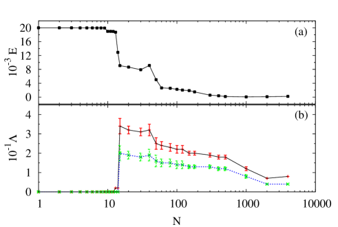
Figure 10: (a) Final time average energy from the system particle and (b) positive LEs as a function of $N$.

both positive LEs increase and the system particle starts to behave chaotically. For higher values of $N$ the LEs decrease slowly [Fig. 10(b)] following the qualitative behavior of the mean final energy [Fig. 10(a)]. It is interesting to observe that very close to the interval of $N$ where the time averaged energy decay emerges ($N=13\rightarrow 15$), both LEs increase and the system dynamics suffer a transition from a regular to a chaotic motion. For higher values of $N$ the final mean energy of the system particle decreases, the LEs decrease, and the motion start to be regular again. This can be seen by comparing Fig. 9(c) with Fig. 10 for $N=4000$, for which the mean final energy is very small and the LEs are close to zero. Since the final energy of the system particle is very small, it will perform small oscillations around the minimum of the potential with a frequency $\omega_{0}$, which is the frequency of the linear motion around the minimum of the potential. Therefore, this harmonic motion induces the regular dynamics. Since all frequencies in this paper are given in units of $\omega_{0}=1.0$, we conclude that for high values of $N$ the system particle oscillate very close to the minimum of the potential with the main frequency close to $w\sim\omega_{0}=1.0$. This is the physical origin of the new frequencies which appear in Fig. 9(c).

From the LEs it is also possible to determine the Kaplan-Yorke dimension ($D_{KY}$). Table 1 shows $D_{KY}$ in the interval $1\leq N\leq 12$ with the corresponding values of $m,~{}\Lambda_{1},~{}\Lambda_{2}$ and $\Lambda_{3}$ (for $m=3$). In the interval $1\leq N\leq 4$ we obtained $D_{KY}\sim 1.0$, for $5\leq N\leq 12$ it is $D_{KY}\sim 2.2$, for $N=13$ it is $D_{KY}\sim 3.94$ and for $N=14$ it is $D_{KY}\sim 3.88$, showing the fractal dimension of the reconstructed attractor and the dissipative behavior of the system particle. For higher values of $N$ we obtained approximately $D_{KY}\sim 4.99$.

Table 1: Kaplan-Yorke dimension ($D_{KY}$) in the interval $1\leq N\leq 12$ with the corresponding Lyapunov spectrum and values of $m$.

$N$	$m$	$\Lambda_{1}$	$\Lambda_{2}$	$\Lambda_{3}$	$D_{KY}$
1	2	0.0001	-0.0023	*****	1.00
2	2	0.0001	-0.0013	*****	1.01
3	2	0.0002	-0.0035	*****	1.01
4	2	0.0012	-0.0057	*****	1.21
5	3	0.0078	-0.0032	-0.0190	2.21
6	3	0.0100	-0.0043	-0.0350	2.16
7	3	0.0097	-0.0042	-0.0215	2.26
8	3	0.0103	-0.0029	-0.0261	2.28
9	3	0.0095	-0.0032	-0.0271	2.23
10	3	0.0096	-0.0047	-0.0255	2.19
11	3	0.0098	-0.0048	-0.0265	2.19
12	3	0.0115	-0.0048	-0.0273	2.25

The main physical process responsible for the regular-chaotic transition occurs due to the overlap of resonances surfaces in the $2N+1$ (constant energy) dimensional space. As the consequence of the KAM (Kolmogorov-Arnold-Moser) theorem [26], it is known that the breakup of tori occurs more likely at resonances between the tori of the unperturbed problem. For $N+1\geq 3$ degrees of freedom, such resonance surfaces are not isolated from each other by the KAM surfaces and they may intersect in the constant energy surface, generating the Arnold web. As $N$ increases, the density of resonance surfaces increases and start to overlap so that a small coupling between the system and environment (the perturbation) is strong enough to breakup the resonant tori, leading to the chaotic motion. This is the reason of the regular-chaotic transition as $N$ increases. Consequently, the motion in Fig. 3 (for $N\gtrsim 13$) comes from the combined effect of chaotic diffusion of trapped trajectories and Arnold diffusion. In Fig. 4 ($N=9$) and Fig. 5 ($N=15$) we observe what happens in the phase-space of the environment oscillators at the regular-chaotic transition. In Fig. 4 all curves are closed giving the impression of a regular motion. For $N=15$ all curves start to display some irregularity. The most perturbed curves occur for $w_{5}$ and $w_{8}$, where the original dynamics in phase space (compare with Fig. 4) is almost destroyed. These are the oscillators with lower frequencies but with larger amplitude of oscillations. Since the coupling between system and environment is bilinear (see Section 2), as the amplitude of the oscillators increases, the perturbation is larger and more likely to induce the chaotic motion (in addition to the overlap of resonances).

Once the chaotic motion is reached, two distinct limit situations can be obtained as $N\rightarrow\infty$, total stochasticity or regular motion [26]. In our case we clearly obtain the regular limit since the LEs decrease as $N\rightarrow 4000$ (confirmed by the power spectrum). As $N$ increases, due to the proximity of resonance surfaces, more and more tori will be broken by the coupling. As a consequence, the trapped trajectory (see discussion related to Fig. 8) will transfer energy to the new degrees of freedom, the LEs will decrease more and more so that for $N\rightarrow 4000$ they are almost zero. Besides that, in the Langevin description (for $N=\infty$), the system particle energy and the energy per oscillators approach zero, and a regular motion is expected. For a more detailed description of overlap of resonances in high-dimensional systems we refer the reader to [26].

5 Conclusions

In this paper we describe the nonlinear behavior of an open system (particle inside the anharmonic potential) interacting with an environment composed of a finite number $N$ of harmonic oscillators. The whole problem (System $+$ Environment $+$ Interaction) is conservative but, due to the energy exchange between system and environment, the system only is considered as an open system with dissipation. Since small dissipation is inevitable in real systems we analyse the nonlinear behavior when the time averaged energy decay of the system particle starts to become relevant. The small dissipation considered here is not modelled by a small damping constant, as usual, but by the finite number $N$ of oscillators. The microscopic dynamics as $N$ increases is not simple and its relation to the macroscopic statistical mechanics is even more complicated.

To determine the values of $N$ where the time averaged energy decay emerges, we analyze the time evolution of the system particle mean energy, which is obtained over $800$ realizations of the environment variables. We show that the time averaged energy for the system particle starts to decay for $N$ in the interval ($10,20$). For lower values of $N$, system and environment just exchange energy and the time average of the mean particle energy remains constant (see Fig. 2 for $N=12$). In the above mentioned interval, the system particle energy starts to be transferred to the environment (see Fig. 2 for $N=13,14$). The transferred energy did not return back to the system for the whole range of integration time. As $N$ increases, the times for which the particles energy is transferred to the environment gets smaller. From the nonlinear analysis we observed that the time series of $X(t)$ for a single trajectory of the system particle dynamics starts to be chaotic for $13\leq N\leq 15$. The power spectra confirm these results. This is exactly the interval of $N$ where the time averaged energy for the system particle starts to decay. For higher values of $N$ the final mean energy of the system particle decreases, the LEs decrease and the motion of the system particle starts to be regular again. This was nicely confirmed with the power spectrum for $N=4000$, shown in Fig. 9(c). In this limit the LEs are close to zero and the system particle energy is very small. The particle oscillates close to the minimum of the anharmonic potential with a frequency close to $w\sim\omega_{0}=1.0$, which is the frequency of the linear motion around the minimum of the potential. We also determined the Kaplan-Yorke dimension, which is $\sim 1.0$ for $1\leq N\leq 4$, $\sim 2.2$ for $5\leq N\leq 12$, $\sim 3.84$ for $13\leq N\leq 15$ and approaches $\sim 4.99$ for $N>15$. Interesting to mention here is that the Kaplan-Yorke dimension is fractal for $5\leq N<15$, typical of dissipative system. Therefore this dimension is not able to recognize that the whole dynamics is conservative. The origin of the chaotic motion is due to the overlap of resonances surfaces in the energy conserving surface as $N$ increases.

The above values of $N$ for which the time averaged energy decay and chaotic motion emerges, are valid for the specific oscillators frequencies generator used in the simulations. These values may change a little if another generator is used [13]. However the qualitative behavior of all analyzed quantities is the same when the time averaged energy starts to decay.

Numerical evidences show a connection between the variation (in time) of the amplitude of the particle energy with the energy decay and the decrease of the Lyapunov exponents. This is explained in terms of chaotic trajectories from the system particles trapped close to regular island. Since this trajectory is restricted to a smaller portion of the phase space, part of the total energy is transferred to other degrees of freedom thus explaining the origin of the time averaged energy decay.

References

- [1] E. Cortés, B. J. West and K. Lindenberg, On The Generalized Langevin Equation - Classical and Quantum-Mechanical, J. Chem. Phys 82 (1985) 2708-2717.
- [2] H. Risken. The Fokker-Planck Equation, Springer-Verlag: Berlin, 1989.
- [3] Y-C Lai, C. Grebogi, Complexity in Hamiltonian-driven dissipative chaotic dynamical systems, Phys. Rev. E 54 (1996) 4667-4675.
- [4] P. C. Rech, M. W. Beims, J. A. C. Gallas, Basin size evolution between dissipative and conservative limits, Phys. Rev. E 71 (2005) 0172021-1-4.
- [5] U. Feudel, C. Grebogi, B. Hunt and J. A. Yorke, Map with more than 100 coexisting low-period periodic attractors, Phys. Rev. E 54 (1996) 71-81.
- [6] A. H. Castro Neto, A. O. Caldeira, New Model for Dissipation in Quantum-Mechanics, Phys. Rev. Lett. 67 (1991) 1960-1963.
- [7] U. Weiss. Quantum Dissipative Systems. World Scientific, Singapore, 1999.
- [8] P. Ullersma, An Exactly Solvable Model for Brownian Motion.I. Derivation of Langevin Equation, Physica 32 (1966) 27-55. R. Zwanzig, Nonlinear generalized Langevin equation, J. Stat. Phys. 9 (1973) 215-220.
- [9] E. Fermi, J. Pasta, M. Tsingou. Los Alamos preprint LA-1940 (1955).
- [10] J. Ford, The Fermi-Pasta-Ulam problem - paradox turns discovery, Phys. Rep. 213 (1992) 271-310.
- [11] H. L. Yang, G. Radons, Hydrodynamic Lyapunov modes and strong stochasticity threshold in Fermi-Pasta-Ulam models, Phys. Rev. E 73 (2006) 016201-1-7. H. L. Yang, G. Radons, Lyapunov instabilities of Lennard-Jones fluids, Phys. Rev. E 71 (2005) 036211-1-15.
- [12] M. V. S. Bonança, M. A. M. de Aguiar, Classical dissipation and asymptotic equilibrium via interaction with chaotic systems, Physica A 365 (2006) 333-350.
- [13] J. Rosa and M. W. Beims. Dissipation and transport dynamics in a Ratchet Coupled to a Discrete Bath, Phys. Rev. E 78, 031126 (2008).
- [14] R. Klages. Microscopic Chaos, Fractals and Transport in Nonequilibrium Statistical Mechanics, World Scientific, London, 2007.
- [15] J. Rosa, M. W. Beims, Environment-dependent transport in multiple asymmetric well potentials, Physica A 342 (2004) 29-33.
- [16] J. Rosa, M. W. Beims, Optimal transport in a Ratchet Coupled to a Modulated Environment: the role of Levy walks, Physica A 386 (2007) 54-62.
- [17] M. Sano, Y. Sawada. Measurement of the Lyapunov spectrum from a chaotic time-series, Phys. Rev. Lett. 55 (1985) 1082-1085.
- [18] R. Hegger, H. Kantz, T. Schreiber, Practical implementation of nonlinear time series methods: The TISEAN package, Chaos 9 (1999) 413-435.
- [19] H. Kantz, T. Schreiber, Nonlinear Time Series Analysis, Cambridge University Press, Cambridge, 1997.
- [20] W. H. Press, S. A. Teukolsky, W.T. Vetterling, B.P. Flannery, Numerical Recipes in Fortran, Cambridge University Press, USA, 1992.
- [21] F. Takens. Dynamical Systems and Turbulence. Lecture Notes in Mathematics; Springer-Verlag: New York; 1981.
- [22] M. B. Kennel, R. Brown, H. D. I. Abarbanel, Determining Embedding dimension for phase-space reconstruction using a geometrical construction, Phys. Rev. A 45 (1992) 3403-3411.
- [23] G. M. Zaslavski, Chaos and fractional kinetics, and anomalous transport, Phys. Rep. 371 (2002) 461-580.
- [24] V. J. Donnay, Non-ergodicity of two particles interacting via a smooth potential, J. Stat. Phys. 96 (1999) 1021-1048.
- [25] M. W. Beims, C. Manchein, J. M. Rost, Origin of chaos in soft interactions and signatures of nonergodicity, Phys. Rev. E 76 (2007) 056203-11;
- [26] A. J. Lichtenberg, M. A. Lieberman, Regular and Chaotic Dynamics, Springer-Verlag, Berlin 1992.