Multiple time scales hidden in heterogeneous dynamics of glass-forming liquids

Abstract

A multi-time probing of density fluctuations is introduced to investigate hidden time scales of heterogeneous dynamics in glass-forming liquids. Molecular dynamics simulations for simple glass-forming liquids are performed, and a three-time correlation function is numerically calculated for general time intervals. It is demonstrated that the three-time correlation function is sensitive to the heterogeneous dynamics and that it reveals couplings of correlated motions over a wide range of time scales. Furthermore, the time scale of the heterogeneous dynamics $\tau_{\rm hetero}$ is determined by the change in the second time interval in the three-time correlation function. The present results show that the time scale of the heterogeneous dynamics $\tau_{\rm hetero}$ becomes larger than the $\alpha$-relaxation time at low temperatures and large wavelengths. We also find a dynamical scaling relation between the time scale $\tau_{\rm hetero}$ and the length scale $\xi$ of dynamical heterogeneity as $\tau_{\rm hetero}\sim\xi^{z}$ with $z=3$.

The understanding of drastic slowing down and non-exponential relaxations in glasses and dense colloids and the jamming of granular materials is one of the most challenging problems in condensed matter physics. Extensive studies have been carried out through experiments, computer simulations, and theories Binder and Kob (2005); Liu and Nagel (2001). Recently, the concept of “dynamical heterogeneity” in glass-forming liquids has attracted much attention and has been considered as an essential notion for understanding the slow dynamics. Near the glass transition temperature, the dynamics becomes spatially heterogeneous and include the coexistence of mobile and immobile correlated regions. A number of molecular dynamics simulations Hurley and Harrowell (1995); Kob et al. (1997); Donati et al. (1998); Muranaka and Hiwatari (1995); Yamamoto and Onuki (1998a, b); Perera and Harrowell (1999); Doliwa and Heuer (2002); Glotzer (2000); Lačević et al. (2003); Berthier (2004) and experiments Kegel and van Blaaderen (2000); Weeks et al. (2000) have detected the existence of dynamical heterogeneity with various visualizations.

To characterize the heterogeneous dynamics in glass-forming liquids, explorations that can provide more detailed information that is not available from conventional two-point correlation functions, are essential and significant. In fact, the growth of the length scale $\xi$ with decreasing temperature has been measured in terms of four-point correlation functions by simulations  Yamamoto and Onuki (1998a, b); Perera and Harrowell (1999); Glotzer (2000); Lačević et al. (2003); Berthier (2004); Toninelli et al. (2005); Chandler et al. (2006); Stein and Andersen (2008), experiments Ediger (2000); Richert (2002); Berthier et al. (2005), and mode-coupling theory Biroli et al. (2006).

Another important issue is the temporal details of the dynamical heterogeneity, such as the lifetime and the relocation time, i.e., the time scale over which slow (fast) moving particles remain slow (fast). The central question is whether or not the lifetime of dynamical heterogeneity $\tau_{\rm hetero}$ is comparable to the so-called $\alpha$-relaxation time $\tau_{\alpha}$ determined by the two-point correlation function Ediger (2000); Richert (2002). If the deviation between the two time scales becomes large near the glass transition temperature, the details of the relaxation processes of spatially heterogeneous dynamics are essential to understanding the drastic slowing down.

In order to quantify $\tau_{\rm hetero}$, a multiple time extension of the density correlation function is necessary, since the two-point correlation function averaging over the full ensemble cannot distinguish among dynamics of sub-ensembles. This idea has been applied to various experiments such as multidimensional nuclear magnetic resonance, hole-burning, and photobleaching Schmidt-Rohr and Spiess (1991); Böhmer et al. (1996); Wang and Ediger (1999, 2000); Ediger (2000); Richert (2002). Recently, several experiments have provided the evidence to support that the lifetime of heterogeneous dynamics $\tau_{\rm hetero}$ becomes larger than the structural relaxation time near the glass transition Wang and Ediger (1999, 2000). In computer simulations, the multiple time extension has also been employed to determine the lifetime of heterogeneous dynamics Heuer and Okun (1997); Heuer (1997); Yamamoto and Onuki (1998b); Doliwa and Heuer (1998); Perera and Harrowell (1999); Doliwa and Heuer (2002); Flenner and Szamel (2004); Léonard and Berthier (2005); Jung et al. (2005). In these calculations, however, due to intense calculations several time intervals are fixed at a characteristic time scale, and thus only limited information on the lifetime of the heterogeneous dynamics has been provided.

In this paper, we present the comprehensive information regarding the lifetime of dynamical heterogeneity and its temperature dependence. We perform molecular dynamics (MD) simulations for simple glass-forming liquids at various temperatures and investigate the dynamics in terms of a multi-time correlation function that shows the coupling of motions with various time scales in the heterogeneous dynamics. The wave vector dependence of the lifetime of heterogeneous dynamics is also studied. Furthermore, the dynamical scaling relation between the lifetime and the length scale of the dynamical heterogeneity is presented.

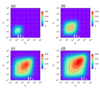
Figure 1: Two-dimensional plots of the three-time correlation function $F_{4}(k,t_{1},t_{2},t_{3})$ of component $1$ particles at waiting time $t_{2}=0$ for various temperatures $T=0.473$ (a), $0.352$ (b), $0.306$ (c), and $0.289$ (d). For each temperature, $\tau_{\alpha}$ is indicated by the arrow. The wave vector $k$ is chosen as $k=2\pi$.

Similar to earlier studies Heuer and Okun (1997); Heuer (1997); Doliwa and Heuer (1998); Flenner and Szamel (2004); Léonard and Berthier (2005), we define the three-time, i.e., four-point, correlation function with times $0$, $\tau_{1}$, $\tau_{2}$, and $\tau_{3}$,

$$F_{4}(k,t_{1},t_{2},t_{3})=\biggl{\langle}\frac{1}{N}\sum_{j=1}^{N}\delta F_{j}(\mbox{\boldmath$k$},\tau_{2},\tau_{3})\delta F_{j}(\bm{k},0,\tau_{1}))\biggr{\rangle},$$ (1)

where $\delta F_{j}(\mbox{\boldmath$k$},0,\tau)=\cos[\mbox{\boldmath$k$}\cdot\Delta\mbox{\boldmath$r$}_{j}(0,\tau)]-F_{s}(k,\tau)$ is the individual fluctuation in the incoherent intermediate scattering function defined as $F_{s}(k,\tau)=\langle(1/N)\sum_{j=1}^{N}\cos(\mbox{\boldmath$k$}\cdot\Delta\mbox{\boldmath$r$}_{j}(0,\tau))\rangle$ with the wave vector $k$ and $k=|\mbox{\boldmath$k$}|$. Here, $\Delta{\mbox{\boldmath$r$}}_{j}(0,\tau)={\mbox{\boldmath$r$}}_{j}(\tau)-{\mbox{\boldmath$r$}}_{j}(0)$ is the displacement vector between two times, $0$ and $\tau$ of $j$-th particle. The $\langle\cdots\rangle$ represents the ensemble average over the initial time $t=0$ and the angular components of the wave vector. The definition of the time interval $t_{i}$ is $t_{i}=\tau_{i}-\tau_{i-1}$, where $\tau_{0}=0$. It is noted that $F_{4}(k,t_{1},t_{2},t_{3})$ expresses the correlations between fluctuations in the two-point correlation function $F_{s}(k,t)$ between two time intervals, $t_{1}=\tau_{1}$ and $t_{3}=\tau_{3}-\tau_{2}$. If the dynamics are homogeneous and if the motions between the two intervals $t_{1}$ and $t_{3}$ are uncorrelated and decoupled, the multi-time correlation function $F_{4}(k,t_{1},t_{2},t_{3})$ should become zero. On the other hand, if the dynamics are heterogeneous, spatially heterogeneous structures governed by the dichotomy between fast- and slow-moving regions lead to finite values of $F_{4}(k,t_{1},t_{2},t_{3})$ due to correlations of motions between the two intervals $t_{1}$ and $t_{3}$. Furthermore, the progressive change in the waiting time $t_{2}=\tau_{3}-\tau_{2}$ of $F_{4}(k,t_{1},t_{2},t_{3})$ enables us to investigate the time scale of the heterogeneous structure in glass-forming liquids. In other words, the first two-point function $\delta F_{j}(\mbox{\boldmath$k$},0,\tau_{1})$ is capable of selecting the sub-ensemble of slow (fast) contributions in heterogeneities and the total function $\delta F_{j}(\mbox{\boldmath$k$},0,\tau_{1})\delta F_{j}(\mbox{\boldmath$k$},\tau_{2},\tau_{3})$ can reveal how long the difference in the dynamics of the sub-ensembles remains over the waiting time $t_{2}$ Heuer (1997). It should be noted that multi-time correlation functions are exploited in nonlinear multidimensional spectroscopic studies of liquids and proteins to understand the detailed dynamics, e.g., the transition from inhomogeneous to homogeneous dynamics and the couplings of molecular motions Mukamel (1999); Hochstrasser (2007).

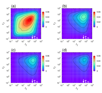
Figure 2: Two-dimensional plots of the three-time correlation function $F_{4}(k,t_{1},t_{2},t_{3})$ of component $1$ particles for $T=0.289$ at several waiting time $t_{2}=0$ (a), $0.5\tau_{\alpha}$ (b), $\tau_{\alpha}$ (c), and $2\tau_{\alpha}$ (d). $\tau_{\alpha}$ is indicated by the arrow. The wave vector $k$ is chosen as $k=2\pi$.

To calculate our three-time correlation function Eq. (1), we have generated long-time trajectories of MD simulations for a glass-forming binary mixture composed of soft sphere components $1$ and $2$. Particles interact via a soft-core potential $v_{ab}(r)=\epsilon(\sigma_{ab}/r)^{12}$, where $\sigma_{ab}=(\sigma_{a}+\sigma_{b})/2$ and $a,b\in\{1,2\}$. The interaction is truncated at $r=3\sigma_{1}$. The size and mass ratio are $\sigma_{1}/\sigma_{2}=1/1.2$ and $m_{1}/m_{2}=1/2$, respectively. The units of length, time, and temperature are $\sigma_{1}$, $\tau_{0}=({m_{1}\sigma_{1}^{2}/\epsilon})^{1/2}$, and $\epsilon/k_{B}$ in this paper. Details of the simulations are given in previous papers Yamamoto and Onuki (1998b, a). The systems are composed of $N=N_{1}+N_{2}=1000$ particles with a fixed density $\rho=N/L^{3}=0.8$ and a composition $N_{1}/N=0.5$. The corresponding system linear dimension is $L=10.8$. Simulations were carried out at various temperatures $T=0.772$, $0.473$, $0.352$, $0.306$, and $0.289$ with a time step $\Delta t=0.005$. Periodic boundary conditions were used in all simulations. At each temperature, the system was carefully equilibrated in the canonical condition, and then, data were taken in the microcanonical condition. We have defined the $\alpha$-relaxation time $\tau_{\alpha}$ for each temperature by $F_{s}(k=2\pi,\tau_{\alpha})=e^{-1}$ for component $1$ particles, where $k=2\pi$ corresponds to the wave vector of the first peak of the static structure factor.

In Fig. 1, we show the two-dimensional plot of $F_{4}(k,t_{1},t_{2},t_{3})$ of component $1$ particles at the zero waiting time, $t_{2}=0$, for various temperatures. $k$ is chosen as $k=2\pi$. It is demonstrated that the intensity of $F_{4}(k,t_{1},t_{2},t_{3})$ grows with decreasing $T$, due to correlated motions of heterogeneous dynamics. This indicates that particles located in slow (fast) moving regions during the first time interval $t_{1}$ tend to remain slow (fast) during the second time interval $t_{3}$. The line shape of $F_{4}(k,t_{1},t_{2},t_{3})$ is seen along the diagonal line $t_{1}=t_{3}$, and the time at which $F_{4}$ has a maximum value is approximately given by the $\alpha$-relaxation time $\tau_{\alpha}$. We here remark that the diagonal part $t_{1}=t_{3}$ at $t_{2}=0$ corresponds to the three-time correlation function used in earlier studies Heuer and Okun (1997); Heuer (1997); Doliwa and Heuer (1998) to judge whether the relaxation type of the dynamics is homogeneous or heterogeneous.

Figure 3: Diagonal part of the three-time correlation function $F_{4}(k,t,t_{2},t)$ of component $1$ particles for $T=0.289$ at various waiting times $t_{2}=0$, $0.5\tau_{\alpha}$, $\tau_{\alpha}$, $2\tau_{\alpha}$, $3\tau_{\alpha}$, $4\tau_{\alpha}$, $6\tau_{\alpha}$, and $10\tau_{\alpha}$ from top to bottom. The wave vector $k$ is chosen as $k=2\pi$. The $\alpha$-relaxation time and the times at which the non-Gaussian parameter $\alpha_{2}(t)$ and the dynamic susceptibility $\chi_{4}(k=2\pi,t)$ reach their peak values are indicated as $\tau_{\alpha}$, $\tau_{\rm NGP}$ and $\tau_{\chi_{4}}$, respectively.

We next investigate how the heterogeneous dynamics evolve with waiting time $t_{2}$. Figure 2 shows that the waiting time dependence of $F_{4}(k,t_{1},t_{2},t_{3})$ at the lower temperature $T=0.289$. In addition, in Fig. 3, we plot the diagonal line along $t_{1}=t_{3}$ of $F_{4}$ at various $t_{2}$ values. It is seen that the correlation gradually decays with increasing the waiting time $t_{2}$ and tends to become zero for $t_{2}\to\infty$. The presence of motions correlated with the $\alpha$-relaxation time scale is clearly observed, even for $t_{2}=10\tau_{\alpha}$. Moreover, the off-diagonal part of $F_{4}$ exists as $t_{2}$ increases. This indicates that motions between the $\alpha$-relaxation and other relaxations with different time scales, such as $\beta$-relaxation, are also coupled, even for large $t_{2}$ values. Here, it is seen in Fig. 3 that the peak position of $F_{4}$ changes slightly with $t_{2}$. For $t_{2}=0$, the peak appears around the time $\tau_{\rm NGP}$, where the non-Gaussian parameter $\alpha_{2}(t)=3\langle\Delta r^{4}(t)\rangle/5\langle\Delta r^{2}(t)\rangle^{2}-1$ has a peak. On the other hand, for large $t_{2}$, we find that the peak of $F_{4}$ tends to shift to the slower time $\tau_{\chi_{4}}$, where the non-linear dynamical susceptibility defined as $\chi_{4}(k,t)=N\langle[(1/N)\sum_{j=1}^{N}\delta F_{j}(\mbox{\boldmath$k$},0,t)]^{2}\rangle$ with $k=2\pi$ has a peak.

Here, we determine the lifetime of heterogeneous dynamics $\tau_{\rm hetero}$ and examine its temperature dependence. As in the previous studies Jung et al. (2005); Léonard and Berthier (2005), we define the volume of $F_{4}(k,t_{1},t_{2},t_{3})$ by integrating over $t_{1}$ and $t_{3}$ as

$$\Delta_{\rm hetero}(k,t_{2})=\int\int F_{4}(k,t_{1},t_{2},t_{3})dt_{1}dt_{3}.$$ (2)

Figure 4 shows $\Delta_{\rm hetero}(k,t_{2})/\Delta_{\rm hetero}(k,0)$ with $k=2\pi$ as a function of the waiting time $t_{2}$ normalized by the $\alpha$-relaxation time $\tau_{\alpha}$. As seen in Fig. 4, $\Delta_{\rm hetero}$ rapidly decays to zero at higher temperatures, and the time scale is comparable to $\tau_{\alpha}$. In contrast, at lower temperatures, the relaxation of $\Delta_{\rm hetero}$ occurs on a time scale larger than $\tau_{\alpha}$. $\Delta_{\rm hetero}(k,t_{2})/\Delta_{\rm hetero}(k,0)$ can be fitted by the stretched-exponential function $\exp[-(t_{2}/\tau_{\rm hetero})^{c}]$, where $\tau_{\rm hetero}$ can be regarded as the lifetime of the heterogeneous dynamics. We plot $\tau_{\rm hetero}$ for each temperature $T$ and wave vector $k$ in Fig. 5. In Fig. 5, it is found that $\tau_{\rm hetero}$ becomes large as the temperature $T$ decreases. In practice, the lifetime $\tau_{\rm hetero}$ is about $6\tau_{\alpha}$ with $c\sim 0.5$ at $T=0.289$ and $k=2\pi$. Furthermore, we confirm that $\tau_{\rm hetero}$ systematically increases with decreasing $k$, implying that couplings of large scale motions have long time scales in heterogeneous dynamics. Such strong deviations and decouplings between $\tau_{\rm hetero}$ and $\tau_{\alpha}$ with decreasing $T$ have been observed in experiments Wang and Ediger (1999, 2000) and simulations Yamamoto and Onuki (1998b); Léonard and Berthier (2005); Hedges et al. (2007). A more recent study has demonstrated that the time scale for Fickian diffusion increases faster than $\tau_{\alpha}$ Szamel and Flenner (2006), which would be related to our results. Another recent study has also mentioned the existence of the slower relaxation time is not $\tau_{\alpha}$, but the lifetime of dynamical heterogeneity Kawasaki and Tanaka (2009).

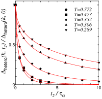
Figure 4: Waiting time $t_{2}$ dependence of the integrated three-time correlation function $\Delta_{\rm hetero}(k,t_{2})/\Delta_{\rm hetero}(k,0)$ for various temperatures. The waiting times are normalized by the $\alpha$ relaxation time $\tau_{\alpha}$ for each temperature. The wave vector $k$ is chosen as $k=2\pi$. The solid curve is determined by fitting with the stretched-exponential form for each temperature.

Finally, it is of great interest to examine the dynamical scaling relation between the time and length scales of dynamical heterogeneity. As is mentioned, the four-point correlation function is used to extract the length scale $\xi$ of the dynamical heterogeneity, where the fluctuation in the two-point correlation function can be considered as an order parameter as seen in critical phenomena. Various dynamical scaling relations have been proposed Yamamoto and Onuki (1998a); Perera and Harrowell (1999); Lačević et al. (2003), however the time scale is practically chosen as the relaxation time of the two-point correlation function, $\tau_{\alpha}$. Here, we note that the time scale associated with $\xi$ should be the average lifetime of the fluctuations in the two-point correlation function, i.e., $\tau_{\rm hetero}$. From the inset of Fig. 5, we observe a quantitative power law behavior between $\tau_{\rm hetero}$ and $\tau_{\alpha}$ as $\tau_{\rm hetero}\sim{\tau_{\alpha}}^{\zeta}$ with $\zeta=1.5$ for $k=2\pi$. A previous study reports that a scaling relation between $\tau_{\alpha}$ and $\xi$ as $\tau_{\alpha}\sim\xi^{z^{\prime}}$ with $z^{\prime}=2$ in the present binary soft sphere system Yamamoto and Onuki (1998a). Note that in Ref. Yamamoto and Onuki (1998a) the correlation length $\xi$ is estimated in terms of the static structure factors of bond breakage processes among adjacent particle pairs, which is essentially the same as the $\xi$ determined by the four-point correlation function consisting of fluctuations in the local mobility Glotzer (2000); Lačević et al. (2003); Berthier (2004); Toninelli et al. (2005); Chandler et al. (2006). Employing this relation, we obtain a new dynamical scaling relation as $\tau_{\rm hetero}\sim\xi^{z}$ with $z=z^{\prime}\zeta=3$, which characterizes the relaxation processes of the dynamical heterogeneity.

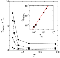
Figure 5: Lifetime of heterogeneous dynamics $\tau_{\rm hetero}$ normalized by the $\alpha$-relaxation $\tau_{\alpha}$ versus temperature $T$ for $k=\pi$ (circles), $2\pi$ (squares), $3\pi$ (diamonds), and $4\pi$ (triangles). Inset: Relation between $\tau_{\rm hetero}$ and $\tau_{\alpha}$ for $k=2\pi$. The straight line with the slope 1.5 is a viewing guide.

In summary, we have investigated a multi-time correlation function to quantitatively characterize the time scale of dynamical heterogeneity. The two-dimensional plots reveal couplings of particle motions with various time scales, and progressive changes in the waiting time allowed us to extract the time scale of heterogeneous dynamics in glass-forming liquids. It is demonstrated that the lifetime of heterogeneous dynamics becomes rapidly larger than the $\alpha$-relaxation time as the temperature decreases, which is compatible with recent optical experimental results Wang and Ediger (1999, 2000) and computer simulation studies Yamamoto and Onuki (1998b); Léonard and Berthier (2005); Szamel and Flenner (2006); Hedges et al. (2007); Kawasaki and Tanaka (2009). We have also studied the wave vector dependence of the lifetime, which is found to systematically increase for large length scales. We have furthermore confirmed the dynamical scaling relation between the time and length scales of dynamical heterogeneity as $\tau_{\rm hetero}\sim\xi^{z}$ with $z=3$, where both variables are determined in terms of the four-point correlation function. It is worth mentioning that the existence of the slower time scale $\tau_{\rm hetero}$ than $\tau_{\alpha}$ may give the new insights into the characterizing of the violation of the Stokes–Einstein relation Yamamoto and Onuki (1998b); Jung et al. (2004); Hedges et al. (2007) and non-Newtonian behaviors in sheared glassy liquids Yamamoto and Onuki (1998a); Furukawa et al. (2009), as is discussed in Ref. Kawasaki and Tanaka (2009).

This work is partially supported by KAKENHI; Young Scientists (B) and Priority Area “Molecular Theory for Real Systems”, the Molecular-Based New Computational Science Program, NINS, and the Next Generation Super Computing Project, Nanoscience program. The computations were performed at RCCS, Okazaki, Japan.

References

- Binder and Kob (2005) K. Binder and W. Kob, Glassy Materials and Disordered Solids (World Scientific, Singapore, 2005).
- Liu and Nagel (2001) A. J. Liu and S. R. Nagel, eds., Jamming and Rheology (Taylor & Francis, New York, 2001).
- Hurley and Harrowell (1995) M. M. Hurley and P. Harrowell, Phys. Rev. E 52, 1694 (1995).
- Kob et al. (1997) W. Kob, C. Donati, S. J. Plimpton, P. H. Poole, and S. C. Glotzer, Phys. Rev. Lett. 79, 2827 (1997).
- Donati et al. (1998) C. Donati, J. F. Douglas, W. Kob, S. J. Plimpton, P. H. Poole, and S. C. Glotzer, Phys. Rev. Lett. 80, 2338 (1998).
- Muranaka and Hiwatari (1995) T. Muranaka and Y. Hiwatari, Phys. Rev. E 51, R2735 (1995).
- Yamamoto and Onuki (1998a) R. Yamamoto and A. Onuki, Phys. Rev. E 58, 3515 (1998a).
- Yamamoto and Onuki (1998b) R. Yamamoto and A. Onuki, Phys. Rev. Lett. 81, 4915 (1998b).
- Perera and Harrowell (1999) D. N. Perera and P. Harrowell, J. Chem. Phys. 111, 5441 (1999).
- Doliwa and Heuer (2002) B. Doliwa and A. Heuer, J. Non-Cryst. Solids 307-310, 32 (2002).
- Glotzer (2000) S. C. Glotzer, J. Non-Cryst. Solids 274, 342 (2000).
- Lačević et al. (2003) N. Lačević, F. W. Starr, T. B. Schrøder, and S. C. Glotzer, J. Chem. Phys. 119, 7372 (2003).
- Berthier (2004) L. Berthier, Phys. Rev. E 69, 020201(R) (2004).
- Kegel and van Blaaderen (2000) W. K. Kegel and A. van Blaaderen, Science 287, 290 (2000).
- Weeks et al. (2000) E. R. Weeks, J. Crocker, A. C. Levitt, A. Schofield, and D. Weitz, Science 287, 627 (2000).
- Toninelli et al. (2005) C. Toninelli, M. Wyart, L. Berthier, G. Biroli, and J. P. Bouchaud, Phys. Rev. E 71, 041505 (2005).
- Chandler et al. (2006) D. Chandler, J. P. Garrahan, R. L. Jack, L. Maibaum, and A. C. Pan, Phys. Rev. E 74, 051501 (2006).
- Stein and Andersen (2008) R. S. L. Stein and H. C. Andersen, Phys. Rev. Lett. 101, 267802 (2008).
- Ediger (2000) M. D. Ediger, Annu. Rev. Phys. Chem. 51, 99 (2000).
- Richert (2002) R. Richert, J. Phys.: Condens. Matt. 14, R703 (2002).
- Berthier et al. (2005) L. Berthier, G. Biroli, J. P. Bouchaud, L. Cipelletti, E. D. Masri, D. L’Hote, F. Ladieu, and M. Pierno, Science 310, 1797 (2005).
- Biroli et al. (2006) G. Biroli, J. P. Bouchaud, K. Miyazaki, and D. R. Reichman, Phys. Rev. Lett. 97, 195701 (2006).
- Schmidt-Rohr and Spiess (1991) K. Schmidt-Rohr and H. W. Spiess, Phys. Rev. Lett. 66, 3020 (1991).
- Böhmer et al. (1996) R. Böhmer, G. Hinze, G. Diezemann, B. Geil, and H. Sillescu, Europhys. Lett. 36, 55 (1996).
- Wang and Ediger (1999) C. Y. Wang and M. D. Ediger, J. Phys. Chem. B 103, 4177 (1999).
- Wang and Ediger (2000) C. Y. Wang and M. D. Ediger, J. Chem. Phys. 112, 6933 (2000).
- Heuer and Okun (1997) A. Heuer and K. Okun, J. Chem. Phys. 106, 6176 (1997).
- Heuer (1997) A. Heuer, Phys. Rev. E 56, 730 (1997).
- Doliwa and Heuer (1998) B. Doliwa and A. Heuer, Phys. Rev. Lett. 80, 4915 (1998).
- Flenner and Szamel (2004) E. Flenner and G. Szamel, Phys. Rev. E 70, 052501 (2004).
- Léonard and Berthier (2005) S. Léonard and L. Berthier, J. Phys.: Condens. Matt. 17, S3571 (2005).
- Jung et al. (2005) Y. J. Jung, J. P. Garrahan, and D. Chandler, J. Chem. Phys. 123, 084509 (2005).
- Mukamel (1999) S. Mukamel, Principles of Nonlinear Optical Spectroscopy (Oxford University Press, USA, 1999).
- Hochstrasser (2007) R. M. Hochstrasser, Proc. Natl. Acad. Sci. U.S.A 104, 14190 (2007).
- Hedges et al. (2007) L. O. Hedges, L. Maibaum, D. Chandler, and J. P. Garrahan, J. Chem. Phys. 127 (2007).
- Szamel and Flenner (2006) G. Szamel and E. Flenner, Phys. Rev. E 73, 011504 (2006).
- Kawasaki and Tanaka (2009) T. Kawasaki and H. Tanaka, Phys. Rev. Lett. 102, 185701 (2009).
- Jung et al. (2004) Y. J. Jung, J. P. Garrahan, and D. Chandler, Phys. Rev. E 69, 061205 (2004).
- Furukawa et al. (2009) A. Furukawa, K. Kim, S. Saito, and H. Tanaka, Phys. Rev. Lett. 102, 016001 (2009).