Dynamic Evolution Model of Isothermal Voids and Shocks

Abstract

We explore self-similar hydrodynamic evolution of central voids embedded in an isothermal gas of spherical symmetry under the self-gravity. More specifically, we study voids expanding at constant radial speeds in an isothermal gas and construct all types of possible void solutions without or with shocks in surrounding envelopes. We examine properties of void boundaries and outer envelopes. Voids without shocks are all bounded by overdense shells and either inflows or outflows in the outer envelope may occur. These solutions, referred to as type $\mathcal{X}$ void solutions, are further divided into subtypes $\mathcal{X}_{\rm I}$ and $\mathcal{X}_{\rm II}$ according to their characteristic behaviours across the sonic critical line (SCL). Void solutions with shocks in envelopes are referred to as type $\mathcal{Z}$ voids and can have both dense and quasi-smooth edges. Asymptotically, outflows, breezes, inflows, accretions and static outer envelopes may all surround such type $\mathcal{Z}$ voids. Both cases of constant and varying temperatures across isothermal shock fronts are analyzed; they are referred to as types $\mathcal{Z}_{\rm I}$ and $\mathcal{Z}_{\rm II}$ void shock solutions. We apply the ‘phase net matching procedure’ to construct various self-similar void solutions. We also present analysis on void generation mechanisms and describe several astrophysical applications. By including self-gravity, gas pressure and shocks, our isothermal self-similar void (ISSV) model is adaptable to various astrophysical systems such as planetary nebulae, hot bubbles and superbubbles in the interstellar medium as well as supernova remnants.

1 Introduction

Voids may exist in various astrophysical cloud or nebula systems of completely different scales, such as planetary nebulae, supernova remnants, interstellar bubbles and superbubbles and so forth. In order to understand the large-scale dynamic evolution of such gaseous systems, we formulate and develop in this paper an isothermal self-similar dynamic model with spherical symmetry involving central expanding voids under the self-gravity. In our dynamic model framework, a void is approximately regarded as a massless region with a negligible gravity on the surrounding gas envelope. With such idealization and simplification in our hydrodynamic equations, a void is defined as a spherical space or volume containing nothing inside. In any realistic astrophysical systems, there are always materials inside voids such as stellar objects and stellar winds or outflows etc. In Section 4.2.3, we shall show that in astrophysical gas flow systems that our isothermal self-similar void (ISSV) solutions are generally applicable, such as planetary nebulae, interstellar bubbles or superbubbles and so on.

Observationally, early-type stars are reported to blow strong stellar winds towards the surrounding interstellar medium (ISM). Hydrodynamic studies on the interaction of stellar winds with surrounding gases have shown that a stellar wind will sweep up a dense circumsteller shell (e.g. Pikel’ner & Shcheglov 1968; Avedisova 1972; Dyson 1975; Falle 1975). Such swept-up density ‘wall’ surrounding a central star thus form interstellar bubbles of considerably low densities inside (e.g. Castor, McCray & Weaver 1975). For example, the Rosette Nebula (NGC 2237, 2238, 2239, 2246) is a vast cloud of dusts and gases spanning a size of $\sim 100$ light years. It has a spectacular appearance with a thick spherical shell of ionized gas and a cluster of luminous massive OB stars in the central region, whose strong stellar winds and intense radiation have cleared a ‘hole’ or ‘cavity’ around the centre and given rise to a thick spherical shell of ionized gases (e.g. Mathews 1966; Dorland, Montmerle & Doom 1986). Weaver et al. (1977) outlined a dynamic theory to explain interstellar bubbles. They utilized equations of motion and continuity with spherical symmetry. They gave an adiabatic similarity solution, which is applicable at early times and also derived a similarity solution including the effect of thermal conduction between the hotter (e.g. $T\approx 10^{6}$K) interior and the colder shell of swept-up ISM. Their solution was also modified to include effects of radiation losses. Weaver et al. (1977) did not consider the self-gravity of gas shell which can be dynamically important for such a large nebula, and therefore possible behaviours of their self-similar solutions were fairly limited. For example, the thickness of the gas shell was limited to $\sim 0.14$ times of the bubble radius. In our model formulation, we ignore the gravity of the central stellar wind region and of star(s) embedded therein. Thus, this central region is treated as a void and we explore the self-similar dynamic behaviours of surrounding gas shell and ISM involving both the self-gravity and thermal pressure. Our ISSV solutions reveal that the gas shell of a cloud can have many more types of dynamic behaviours.

Planetary nebulae (PNe) represent an open realm of astrophysical applications of our ISSV model, especially for those that appear grossly spherical (e.g. Abell 39; see also Abell 1966). During the stellar evolution, planetary nebulae emerge during the transition from the asymptotic giant branch (AGB) phase where the star has a slow AGB dense wind to a central compact star (i.e. a hot white dwarf) where it blows a fast wind in the late stage of stellar evolution (e.g. Kwok, Purton & Fitzgerald 1978; Kwok & Volk 1985; Chevalier 1997a). The high temperature of the compact star can be a source of photoionizing radiation and may partially or completely photoionize the dense slower wind. Chevalier (1997a) presented an isothermal dynamical model for PNe and constructed spherically symmetric global hydrodynamic solutions to describe the expansion of outer shocked shell with an inner contact discontinuity of wind moving at a constant speed. In Chevalier (1997a), gravity is ignored and the gas flow in the outer region can be either winds or breezes. In this paper, we regard the inner expansion region of fast wind as an effective void and use ISSV solutions with shocks to describe dense shocked wind and AGB wind expansion. One essential difference between our ISSV model and that of Chevalier (1997a) lays in the dynamic behaviour of the ISM. In Chevalier (1997a), shocked envelope keeps expanding with a vanishing terminal velocity or a finite terminal velocity at large radii. By including the self-gravity, our model can describe a planetary nebula expansion surrounded by an outgoing shock which further interacts with a static, outgoing or even accreting ISM. In short, the gas self-gravity is important to regulate dynamic behaviours of a vast gas cloud. Quantitative calculations also show that the lack of gas self-gravity may lead to a considerable difference in the void behaviours (see Section 4.1). Likewise, our ISSV model provides more sensible results than those of Weaver et al. (1977). We also carefully examine the inner fast wind region and show that a inner reverse shock must exist and the shocked fast wind has a significant lower expansion velocity than the unshocked innermost fast wind. It is the shocked wind that sweeps up the AGB slow wind, not the innermost fast wind itself. This effect is not considered in Chevalier (1997a). We also compare ISSV model with Hubble observations on planetary nebula NGC 7662 and show that our ISSV solutions are capable of fitting gross features of PNe.

Various aspects of self-similar gas dynamics have been investigated theoretically for a long time (e.g. Sedov 1959; Larson 1969a, 1969b; Penston 1969a, 1969b; Shu 1977; Hunter 1977, 1986; Landau & Lifshitz 1987; Tsai & Hsu 1995; Chevalier 1997a; Shu et al 2002; Lou & Shen 2004; Bian & Lou 2005). Observations also show that gas motions of this kind of patterns may be generic. Lou & Cao (2008) illustrated one general polytropic example of central void in a self-similar expansion as they explored self-similar dynamics of a relativistically hot gas with a polytropic index $4/3$ (Goldreich & Weber 1980; Fillmore & Goldreich 1984). The conventional polytropic gas model of Hu & Lou (2008) considered expanding central voids embedded in “champagne flows” of star forming clouds and provided versatile solutions to describe dynamic behaviours of “champagne flows” in H II regions (e.g. Alvarez et al. 2006). In this paper, we systematically explore isothermal central voids in self-similar expansion and present various forms of possible ISSV solutions. With gas self-gravity and pressure, our model represents a fairly general theory to describe the dynamic evolution of isothermal voids in astrophysical settings on various spatial and temporal scales.

This paper is structured as follows. Section 1 is an introduction for background information, motivation and astrophysical voids on various scales. Section 2 presents the model formulation for isothermal self-similar hydrodynamics, including the self-similar transformation, analytic asymptotic solutions and isothermal shock conditions. Section 3 explores all kinds of spherical ISSV solutions constructed by the phase diagram matching method with extensions of the so-called “phase net”. In Section 4, we demonstrate the importance of the gas self-gravity, propose the physics on void edge and then give several specific examples that the ISSV solutions are applicable, especially in the contexts of PNe and interstellar bubbles. Conclusions are summarized in Section 5. Technical details are contained in Appendices A and B.

2 Hydrodynamic Model Formulation

We recount basic nonlinear Euler hydrodynamic equations in spherical polar coordinates $(r,\theta,\varphi)$ with self-gravity and isothermal pressure under the spherical symmetry.

2.1 Nonlinear Euler Hydrodynamic Equations

The mass conservation equations simply read

$$\frac{\partial M}{\partial t}+u\frac{\partial M}{\partial r}=0\ ,\\ \qquad\frac{\partial M}{\partial r}=4\pi r^{2}\rho\ ,$$ (1)

where $u$ is the radial flow speed, $M(r,\ t)$ is the enclosed mass within radius $r$ at time $t$ and $\rho(r,\ t)$ is the mass density. The differential form equivalent to continuity equation (1) is

$$\frac{\partial\rho}{\partial t}+\frac{1}{r^{2}}\frac{\partial}{\partial r}(r^{2}\rho u)=0\ .$$ (2)

For an isothermal gas, the radial momentum equation is

$$\frac{\partial u}{\partial t}+u\frac{\partial u}{\partial r}=-\frac{a^{2}}{\rho}\frac{\partial\rho}{\partial r}-\frac{GM}{r^{2}}\ ,$$ (3)

where $G\equiv 6.67\times 10^{-8}$ dyn cm² g^-2 is the gravitational constant, $a\equiv(p/\rho)^{1/2}=(k_{\rm B}T/m)^{1/2}$ is the isothermal sound speed and $p$ is the gas pressure, $k_{\rm B}\equiv 1.38\times 10^{-16}\hbox{ erg K}^{-1}$ is Boltzmann’s constant, $T$ is the constant gas temperature throughout and $m$ is the mean particle mass. Meyer (1997) and Chevalier (1997a) ignored the gas self-gravity in the momentum equation.

A simple dimensional analysis for equations $(\ref{MCE})-(\ref{ME})$ gives an independent dimensionless similarity variable

$$x={r}/{(at)}\ ,$$ (4)

involving the isothermal sound speed $a$. The consistent similarity transformation is then

$$\rho(r,\ t)=\alpha(x)/(4\pi Gt^{2})\ ,\\ M(r,\ t)=a^{3}tm(x)/G\ ,\qquad u(r,\ t)=av(x)\ ,\\$$ (5)

where $\alpha(x)$, $m(x)$, $v(x)$ are the dimensionless reduced variables corresponding to mass density $\rho(r,t)$, enclosed mass $M(r,t)$ and radial flow speed $u(r,t)$, respectively. These reduced variables depend only on $x$ (Shu 1977; Hunter 1977; Whitworth & Summers 1985; Tsai & Hsu 1995; Shu et al 2002; Shen & Lou 2004; Lou & Shen 2004; Bian & Lou 2005). Meyer (1997) adopts a different self-similar transformation by writing $\rho=\bar{\rho}(x)/r^{2}$. By equation (4) above, we know that in Meyer (1997), $\bar{\rho}(x)$ is exactly equal to $x^{2}\alpha(x)a^{2}/(4\pi G)$ here. So the similarity transformation of Meyer (1997) is equivalent to similarity transformation (5) here but without the self-gravity. Further analysis will show that transformation (5) can satisfy the void boundary expansion requirement automatically (see Section 4.2.1).

With self-similar transformation (4) and (5), equation (1) yields two ordinary differential equations (ODEs)

$$m+(v-x)\frac{dm}{dx}=0\ ,\qquad\qquad\frac{dm}{dx}=x^{2}\alpha\ .$$ (6)

The derivative term $dm/dx$ can be eliminated from these two relations in equation (6) to give

$$m(x)=x^{2}\alpha(x-v)\ .$$ (7)

A nonnegative mass $m(x)$ corresponds to $x-v>0$. In figure displays of $-v(x)$ versus $x$ profiles, the lower left portion to the line $v-x=0$ is thus unphysical. We refer to the line $v-x=0$ as the “Zero Mass Line” (ZML); inside of $x=v$, there should be no mass, corresponding to a void.

Relation (7) plus transformation (4) and (5) lead to two coupled ODEs from equations (2) and (3), namely

$$\left[(x-v)^{2}-1\right]\frac{dv}{dx}=\left[\alpha(x-v)-\frac{2}{x}\right](x-v)\ ,$$ (8)

$$\left[(x-v)^{2}-1\right]\frac{1}{\alpha}\frac{d\alpha}{dx}=\left[\alpha-\frac{2}{x}(x-v)\right](x-v)\$$ (9)

(Shu 1977). ODEs (8) and (9) differ from eqs (3) and (4) of Chevalier (1997a) by including the self-gravity effect.

For ODEs (8) and (9), the singularity at $(x-v)^{2}=1$ corresponds to two parallel straight lines in the diagram of $-v(x)$ versus $x$, representing the isothermal sonic critical lines (SCL) (e.g. Shu 1977; Whitworth & Summers 1985; Tsai & Hsu 1995; Shu et al. 2002; Lou & Shen 2004; Bian & Lou 2005). As $x-v=-1<0$ is unphysical for a negative mass, we have the SCL characterized by

$$\qquad v=x-1\ ,\\ \alpha={2}/{x}\ .$$ (10)

Two important global analytic solutions of nonlinear ODEs (8) and (9) are the static singular isothermal sphere (SIS; e.g. Shu 1977)

$$v=0\ ,\qquad\qquad\alpha=\frac{2}{x^{2}}\ ,\qquad\qquad m=2x\ ,$$ (11)

and non-relativistic Einstein-de Sitter expansion solution for an isothermal gas

$$v=\frac{2}{3}x\ ,\qquad\alpha=\frac{2}{3}\ ,\qquad m=\frac{2}{9}x^{3}\$$ (12)

(e.g. Whitworth & Summers 1985; Shu et al. 2002).

Let $x_{*}$ denote the value of $x$ at a sonic point on SCL. A Taylor series expansion of $v(x)$ and $\alpha(x)$ in the vicinity of $x_{*}$ shows that solutions crossing the SCL smoothly at $x_{*}$ have the form of either

$$-v=(1-x_{*})+\bigg{(}{1\over x_{*}}-1\bigg{)}(x-x_{*})+\cdots\ ,$$ (13)

$$\alpha={2\over x_{*}}-{2\over x_{*}}\bigg{(}{3\over x_{*}}-1\bigg{)}(x-x_{*})+\cdots\ ,$$

or

$$-v=(1-x_{*})-{1\over x_{*}}(x-x_{*})+\cdots\ ,$$ (14)

$$\alpha={2\over x_{*}}-{2\over x_{*}}(x-x_{*})+\cdots\ ,$$

(e.g. Shu 1977; Whitworth & Summers 1985; Tsai & Hsu 1995; Bian & Lou 2005; see Appendix A of Lou & Shen 2004 for higher-order derivatives). Thus eigensolutions crossing the SCL smoothly are uniquely determined by the value of $x_{*}$. Eigensolutions of type 1 and 2 are defined by equations (13) and (14). Physically, equations (13) and (14) describe how the gas behaves as it flows from subsonic to supersonic regimes across the SCL in the local comoving framework.

An important numerical solution to ODEs (8) and (9) is the Larson-Penston (LP) solution (Larson 1969a; Larson 1969b; Penston 1969). This solution have an asymptotic behaviour $v\rightarrow 2x/3$ and $\alpha\rightarrow 1.67$ as $x\rightarrow 0^{+}$. And the LP solution is also an eigensolution of type 2 (equation 14) and passes through the SCL smoothly at $x_{*}=2.33$.

When $x\rightarrow+\infty$, either at large radii or at very early time, solutions to two nonlinear ODEs (8) and (9) have asymptotic behaviours

$$v=V+\frac{2-A}{x}+\frac{V}{x^{2}}+\frac{(A/6-1)(A-2)+2V^{2}/3}{x^{3}}+\cdots\ ,\\ \alpha=\frac{A}{x^{2}}+\frac{A(2-A)}{2x^{4}}+\frac{(4-A)VA}{3x^{5}}+\cdots\ ,\\ m=Ax-AV+\frac{A(2-A)}{2x}+\frac{A(A-4)V}{6x^{2}}+\cdots\ ,\\$$ (15)

where $V$ and $A$ are two integration constants (e.g. Whitworth & Summers 1985; Lou & Shen 2004), referred to as the reduced velocity and mass parameters, respectively. The non-relativisitic Einstein-de Sitter expansion solution does not follow this asymptotic solution (15) at large $x$. Chevalier (1997a) also presented asymptotic solutions of $v(x)$ and $\alpha(x)$ at large $x$. Case $A=1$ in our solution (15) should correspond to asymptotic behaviours of $v(x)$ and $\alpha(x)$ in Chevalier’s model (1997a; see his equations 5 and 6). However, the coefficient of $x^{-4}$ term for $\alpha(x)$ in his model is $1$ while in our model, it is $1/2$; and coefficient of $x^{-1}$ term for $v(x)$ in his model is $2$ while in our model, it is $2-A$. These differences arise by dropping the gravity in Chevalier (1997a). Physically in our model, the gas has a slower outgoing radial velocity and the density decreases more rapidly than that of Chevalier (1997a), because when the self-gravity is included, the gas tends to accumulate around the centre.

Counterpart solutions to equations (11)$-$(15) can also be generalized for conventional and general polytropic gases (Lou & Wang 2006; Wang & Lou 2007; Lou & Cao 2008; Wang & Lou 2008; Hu & Lou 2008).

2.2 Isothermal Shock Jump Conditions

For an isothermal fluid, the heating and driving of a cloud or a progenitor star (such as a sudden explosion of a star) at $t=0$ will compress the surrounding gas and give rise to outgoing shocks (e.g. Tsai & Hsu 1995). In the isothermal approximation, the mass and momentum should be conserved across a shock front in the shock comoving framework of reference

$$\rho_{d}(u_{d}-u_{s})=\rho_{u}(u_{u}-u_{s})\ ,$$ (16)

$$a_{d}^{2}\rho_{d}+\rho_{d}u_{d}(u_{d}-u_{s})=a_{u}^{2}\rho_{u}+\rho_{u}u_{u}(u_{u}-u_{s})\ ,$$ (17)

where subscripts $d$ and $u$ denote the downstream and upstream sides of a shock, respectively (e.g. Courant & Friedricks 1976; Spitzer 1978; Dyson & Williams 1997; Shen & Lou 2004; Bian & Lou 2005). Physically, we have $u_{s}=a_{d}x_{sd}=a_{u}x_{su}=r_{s}/t$ as the outgoing speed of a shock with $r_{s}$ being the shock radius. Conditions (18) and (19) below in terms of self-similar variables are derived from conditions (16) and (17) by using the reduced variables $v(x)$, $x$ and $\alpha(x)$ and the isothermal sound speed ratio $\tau\equiv a_{d}/a_{u}=x_{su}/x_{sd}$,

$$\alpha_{d}/\alpha_{u}=(v_{u}-x_{su})/[\tau(v_{d}-x_{sd})]\ ,$$ (18)

$$v_{d}-x_{sd}-\tau(v_{u}-x_{su})=(\tau v_{d}-v_{u})(v_{u}-x_{su})(v_{d}-x_{sd})\ .$$ (19)

Consequently, we have $\tau=(T_{d}/T_{u})^{1/2}$ with $T$ being the gas temperature. Physics requires $T_{d}\geq T_{u}$ leading to $\tau\geq 1$. For $\tau=1$, conditions (18) and (19) reduce to

$$\alpha_{d}/\alpha_{u}=(v_{u}-x_{s})/(v_{d}-x_{s})\ ,$$ (20)

$$(v_{u}-x_{s})(v_{d}-x_{s})=1\ ,$$ (21)

where $x_{s}=x_{u}=x_{d}$ is the reduced shock location or speed (e.g. Tsai & Hsu 1995; Chevalier 1997a; Shu et al. 2002; Shen & Lou 2004; Bian & Lou 2005).

3 Isothermal Self-Similar Voids

Various similarity solutions can be constructed to describe outflows (e.g. winds and breezes), inflows (e.g. contractions and accretions), static outer envelope and so forth. These solutions will be presented below in order, as they are useful to construct ISSV solutions.

3.1 Several Relevant Self-Similar Solutions

We first show some valuable similarity solutions in reference to earlier results of Shu (1977) and Lou & Shen (2004). These solutions behave differently as $x\rightarrow+\infty$ for various combinations of parameters $V$ and $A$ in asymptotic solution (15).

3.1.1 CSWCP and EWCS Solutions of Shu (1977)

Shu (1977) presents a class of solutions: collapse solutions without critical point (CSWCP) and expansion-wave collapse solution (EWCS) (see Fig. 1).

The CSWCP solutions (light dotted curves in Fig. 1) have asymptotic behaviours of $V=0$ and $A>2$ according to solution (15) at large $x$, and describe the central free-fall collapse of gas clouds with contracting outer envelopes of vanishing velocities at large radii.

The EWCS solution (the heavy solid curve in Fig. 1) is obtained with $A\rightarrow 2^{+}$ and $V=0$ in solution (15). This solution is tangent to the SCL at $x_{*}=1$ and has an outer static SIS envelope (solution 11) and a free-fall collapse towards the centre ( Shu 1977; Lou & Shen 2004; Bian & Lou 2005); the central collapsed region expands in a self-similar manner.

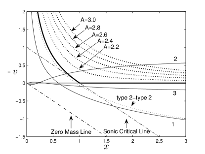
Figure 1: Isothermal self-similar solutions of Shu (1977): $-v(x)$ versus $x$ profile of EWCS (heavy solid curve) and a sequence of five CSWCP solutions (dotted curves) with mass parameter $A$ values marked along these five curves ($A=2.2$ to 3.0). Four solutions smoothly crossing the SCL (dash-dotted line to the upper right) twice of Lou & Shen (2004): three light solid curves labelled by numerals ‘1’, ‘2’ and ‘3’ are type 2-type 1 solutions with their smaller crossing points $x_{*}(1)$ matching the type 2 derivative and the larger crossing points $x_{*}(2)$ fitting the type 1 derivative. The light dotted curve labelled by ‘type 2-type 2’ is the unique type 2-type 2 solution with both crossing points following the type 2 derivative (see Table 1 for relevant parameters). The dash-dotted line to the lower left is the ZML of $x-v=0$.

3.1.2 Solutions smoothly crossing the SCL twice

Lou & Shen (2004) studied isothermal similarity solutions and divided Class I similarity solutions, which follow free-fall behaviours as $x\rightarrow 0^{+}$, into three subclasses according to their behaviours at large $x$. Class Ia similarity solutions have positive $V$ at large $x$ (see solution 15), which describe a cloud with an envelope expansion. Class Ia solutions are referred to as ‘envelope expansion with core collapse’ (EECC) solutions by Lou & Shen (2004). The case of $V=0$ corresponds to Class Ib solutions and $V<0$ renders Class Ic solutions. The CSWCP solutions belong to Class Ic and the EWCS solution belongs to Class Ib.

Lou & Shen (2004) constructed four discrete solutions crossing the SCL twice smoothly (i.e. satisfying equations 13 and 14) by applying the phase diagram matching scheme (Hunter 1977; Whitworth & Summers 1985; see subsection 3.4 below). These are the first four examples among an infinite number of discrete solutions (see Lou & Wang 2007).

Let $x_{*}(1)$ and $x_{*}(2)$ be the smaller (left) and larger (right) cross points for each of the four solutions. As they are all Class I solution, $x_{*}(1)$ is less than $1$ and the behaviours near $x_{*}(1)$ are determined by type 2 (as defined by equation 14) to assure a negative derivative $d(-v)/dx$ at $x_{*}(1)$ along the SCL. As in Lou & Shen (2004), we name a solution that crosses the SCL twice smoothly as ‘type2-type1’ or ‘type2-type2’ solution, which corresponds the derivative types at $x_{*}(1)$ and $x_{*}(2)$. Three of the four solutions of Lou & Shen (2004) are ‘type2-type1’ solutions and we further name them as ‘type2-type1-1’, ‘type2-type1-2’ and ‘type2-type1-3’ (see Fig. 1 and Table 1 for more details).

Table 1: Relevant parameters are summarized here for the four solutions crossing the SCL twice shown in Figure 1. Three of them cross the SCL at $x_{*}(1)$ with the second kind of derivative and at $x_{*}(2)$ with the first kind of derivative. In the ‘Solution’ column of this table, they are named as ‘type2-type1-1’, ‘type2-type1-2’ and ‘type2-type1-3’ corresponding to the curves labelled by ‘1’, ‘2’ and ‘3’, respectively. The fourth solution crosses the SCL at $x_{*}(1)$ and $x_{*}(2)$ both with the second kind of derivative and is named as ‘type2-type2’ in the ‘Solution’ column, corresponding to the curve labelled by ‘type 2-type 2’. The first and third type2-type1 solutions and type2-type2 solution all belong to EECC solution (or Class Ia solution), while the type2-type1-2 solution belongs to Class Ic solution. In Lou & Shen (2004), this type2-type2 EECC solution passes the SCL at $x_{*}(1)\approx 0.632$ and $x_{*}(2)\approx 1.349$. We reproduce these results. However, we here adopt $x_{*}(1)\approx 0.71$ and $x_{*}(2)\approx 1.287$, which are calculated with a higher accuracy.

  Solution Class $x_{*}(1)$ $x_{*}(2)$ $V$ $A$ type2-type1-1 EECC(Ia) $0.23$ $1.65$ $1.8$ $5.1$ type2-type1-2 Ic $2.5858\times 10^{-4}$ $0.743$ $-0.77$ $1.21$ type2-type1-3 EECC(Ia) $6\times 10^{-6}$ $1.1$ $0.3$ $2.4$ type2-type2 EECC(Ia) $0.71$ $1.287$ $1.5$ $4.7$  

3.2 Isothermal Self-Similar Void (ISSV) Solutions

Relation (7) indicates that the ZML $v-x=0$ separates the solution space into the upper-right physical part and the lower-left unphysical part in a $-v(x)$ versus $x$ presentation.

For a solution (with $x-v>0$) touching the ZML at $x_{0}$, then $v(x_{0})=x_{0}$ holds on and so does $m(x_{0})=0$ there. Given the definitions of $m(x)\equiv GM(r,\ t)/(a^{3}t)$ and $x\equiv r/(at)$, condition $m(x_{0})=0$ indicates a spherical isothermal gas whose enclosed mass $M(atx_{0},t)$ vanishes, and thus a central void expands at a constant radial speed $ax_{0}$.

The condition $v(x_{0})=x_{0}$ marks a void boundary in expansion. Physically, $x_{0}$ is the start point of a streamline as $v(x_{0})=x_{0}$ indicates matters flowing outwards at a velocity of the boundary expansion velocity. However, a problem would arise when the gas density just outside the void boundary is not zero. For an isothermal gas, the central vacuum cannot resist an inward pressure from the outer gas across the void boundary. We propose several mechanisms/scenarios to provide sufficient energy and pressure to generate voids and maintain them for a period of time without invalidating our ‘vacuum approximation’ for voids. In Section 4, we present explanations and quantitative calculations about these mechanisms.

Mathematically, to construct spherical isothermal self-similar voids is to search for global solutions reaching the ZML at $x_{0}>0$. If a solution touches the ZML at point $x_{0}$, then $x_{0}$ should be the smallest point of the solution with gas. Solutions with a negative mass are unphysical. So if $v=x$ holds on at $x_{0}$, both $v(x)$ and $\alpha(x)$ should be zero in the range $0<x<x_{0}$.

Before exploring isothermal self-similar void (ISSV) solutions of spherical symmetry, we note a few properties of such solutions. Nonlinear ODEs (8) and (9) give the following two first derivatives at $x_{0}$

$$\frac{dv}{dx}\bigg{|}_{x_{0}}=0\ ,\qquad\qquad\frac{d\alpha}{dx}\bigg{|}_{x_{0}}=0\ .$$ (22)

So in the $-v(x)$ versus $x$ and $\alpha(x)$ versus $x$ presentations, the right tangents to these solution curves at $x_{0}$ are horizontal.

For spherical isothermal self-similar dynamics, we can show that across a void boundary, $\alpha(x)$ must jump from $0$ to a nonzero value (see Appendix A). Voids must be bounded by relatively dense shells with a density jump. We propose that the height of such a density jump may indicate the energy to generate and maintain such a void. Energetic processes of short timescales include supernovae involving rebound shock waves or neutrino emissions and driving processes of long timescales include powerful stellar winds (see Section 4 for more details). In reality, we do not expect an absolute vacuum inside a void. Regions of significantly lower density in gas clouds are usually identified as voids.

For $x\rightarrow+\infty$, the physical requirement of finite mass density and flow velocity can be met for $\alpha(x)$ and $v(x)$ by asymptotic solution (15).

ISSV solutions need to cross the SCL in the $-v(x)$ versus $x$ profiles as they start at the ZML and tend to a horizontal line at large $x$ with a constant $V$. Given conditions (13) and (14), ISSV solutions can be divided into two subtypes: crossing the SCL smoothly without shocks, which will be referred to as type $\mathcal{X}$, and crossing the SCL via shocks, which will be referred to as type $\mathcal{Z}$ and can be further subdivided into types $\mathcal{Z}_{\rm I}$ and $\mathcal{Z}_{II}$ as explained presently.

3.3 Type $\mathcal{X}$ ISSV Solutions without Shocks

As analyzed in Section 3.2, type $\mathcal{X}$ ISSV solutions cross the SCL smoothly. Let $x_{*}$ denote the cross point on the SCL. We have $v(x_{*})=x_{*}-1$ and $\alpha(x_{*})=2/x_{*}$ by equation (10). Conditions (13) and (14) give the eigen solutions for the first derivatives $v^{\prime}(x)$ and $\alpha^{\prime}(x)$ at $x_{*}$ as either type 1 (equation 13) or type 2 (equation 14). Given $x_{*}$ and the type of eigen-derivative at $x_{*}$, all the necessary initial conditions [$v(x_{*})$, $\alpha(x_{*})$, $v^{\prime}(x_{*})$, $\alpha^{\prime}(x_{*})$] are available for integrating nonlinear ODEs (8) and (9) in both directions.

We use $x_{0}$, $\alpha_{0}\equiv\alpha(x_{0})$, $x_{*}$ and the types of eigen-derivative at $x_{*}$ to construct type $\mathcal{X}$ ISSV solutions. While $x_{0}$ and $\alpha_{0}$ are the key parameters for the void expansion speed and the density of the shell around the void edge, we use $x_{*}$ to obtain type $\mathcal{X}$ ISSV solutions as $x_{*}$ parameter can be readily varied to explore all type $\mathcal{X}$ ISSV solutions.

3.3.1 Type $\mathcal{X}_{\rm I}$ ISSV Solutions: Voids with Sharp Edge, Smooth Envelope and Type 1 Derivative on the SCL

Type $\mathcal{X}_{\rm I}$ solutions cross the SCL smoothly and follow the Type 1 derivative at $x_{*}$ on the SCL. By equation (13), the first derivative $d(-v)/dx$ is positive for $0<x_{*}<1$ and negative for $x_{*}>1$. This allows the $x_{*}$ of type $\mathcal{X}_{\rm I}$ solutions to run from $0$ to $+\infty$ when behaviours of these solutions in the inner regions are ignored temporarily. When the existence of $x_{0}$ is required for constructing isothermal central voids, the range of $x_{*}$ along the SCL is then restricted.

Given $x_{*}$ on the SCL and using equations (10) and (13), we obtain the initial condition $v(x_{*}),\ \alpha(x_{*}),\ v^{\prime}(x_{*})$, $\alpha^{\prime}(x_{*})$ to integrate ODEs (8) and (9) from $x_{*}$ in both directions. If an integration towards small $x$ can touch the ZML at a $x_{0}>0$ and an integration towards $+\infty$ exists, then a type $\mathcal{X}_{\rm I}$ ISSV solution is constructed.

We now list five important numerals: $x_{1}\approx 0.743$, $x_{2}=1$, $x_{3}\approx 1.1$, $x_{4}\approx 1.65$ and $x_{5}=3$. They are the cross points at the SCL of Lou & Shen type2-type1-2, SIS (see equation 11), Lou & Shen type2-type1-3, Lou & Shen type2-type1-1, Einstein-de Sitter solution, respectively. All these solutions have type 1 derivatives near their cross points on the SCL. However, their behaviours differ substantially as $x\rightarrow 0^{+}$. The three solutions of Lou & Shen approach central free-fall collapses with a constant reduced core mass $m_{0}$ as the central mass accretion rate; while SIS and Einstein-de Sitter solution have vanishing velocities as $x\rightarrow 0^{+}$.

Numerical computations show that type $\mathcal{X}_{\rm I}$ ISSV solutions exist when $x_{*}$ falls into four intervals out of six intervals along $x>0$ axis divided by the five numerals above. The four intervals are $0<x_{*}<x_{1}\approx 0.743$, $x_{1}\approx 0.743<x_{*}<x_{2}=1$, $x_{2}=1<x_{*}<x_{3}\approx 1.1$ and $x_{3}\approx 1.1<x_{*}<x_{4}\approx 1.65$. No type $\mathcal{X}_{\rm I}$ exist with $x_{*}$ in intervals $x_{4}\approx 1.65<x_{*}<x_{5}=3$ and $x_{*}>x_{5}=3$, because integrations from $x_{*}$ in these two intervals towards $+0$ or $+\infty$ must halt when they encounter the SCL again, respectively. The six regions mentioned above are named as conditions I, II, III, IV, V and VI, respectively. Figure 2 illustrates several typical type $\mathcal{X}_{\rm I}$ ISSV solutions with their $x_{*}$ in different regions. The relevant solution parameters are summarized in Table 2.

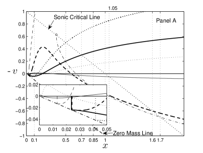
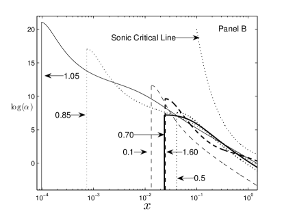
Figure 2: Typical type $\mathcal{X}_{\rm I}$ ISSV solutions. Panel A in linear scales shows $-v(x)$ versus $x$ curves of several type $\mathcal{X}_{\rm I}$ solutions. The sonic critical point $x_{*}$ of each curve is noted along the $x-$axis. The dash-dotted curve which crosses the SCL at $x_{*}=1.7$ smoothly and encounters the line again at $\sim 0.4$ shows a typical behaviour when $x_{4}\approx 1.65<x_{*}<x_{5}=3$. The inset shows the enlarged portions of these ISSV solution curves near $x\rightarrow 0^{+}$. The dash-dotted lines in both panel A and inset are the ZML. Panel B shows the $\log\alpha$ versus $x$ curves of the same solutions and the curves in panel A, inset and panel B with the same line type (light and heavy solid, dotted and dash) correspond to the same type $\mathcal{X}_{\rm I}$ solutions. They are distinguished by their $x_{*}$ values. Each of these curves jumps from a zero value (left) to a nonzero value (right) at $x_{0}$, indicating a void in the region of $x<x_{0}$.

Table 2: Parameters of several typical type $\mathcal{X}_{\rm I}$ ISSV solutions. Eight solutions under four different conditions discussed in Section 3.3.1 are tabulated here.

  Condition $x_{*}$ $x_{0}$ $\alpha_{0}$ $V$ $A$ I $0.10$ $0.0132$ $1.11\times 10^{5}$ $-3.51$ $0.070$ I $0.50$ $0.0417$ $1.92\times 10^{3}$ $-1.57$ $0.649$ I $0.70$ $0.0238$ $1.35\times 10^{3}$ $-0.91$ $1.10$ II $0.75$ $7.5\times 10^{-5}$ $1.5\times 10^{10}$ $-0.75$ $1.23$ II $0.85$ $7.5\times 10^{-4}$ $2.5\times 10^{7}$ $-0.46$ $1.50$ II $0.95$ $5.6\times 10^{-4}$ $6.9\times 10^{6}$ $-0.15$ $1.83$ III $1.05$ $9.2\times 10^{-5}$ $1.5\times 10^{9}$ $+0.14$ $2.17$ IV $1.60$ $0.0242$ $1.5\times 10^{4}$ $+1.71$ $4.77$  

3.3.2 Type $\mathcal{X}_{\rm II}$ Void Solutions: Voids with Sharp Edges, Smooth Envelope and Type 2 Derivative at the SCL

Type $\mathcal{X}_{\rm II}$ solutions cross the SCL smoothly and have the type 2 derivative at $x_{*}$. By condition (14), the first derivative $d(-v)/dx$ is negative for $x_{*}>0$. Because $x_{0}<x_{*}$, $x_{*}$ of type $\mathcal{X}_{\rm II}$ solutions must be larger than $1$ to assure behaviours of solution (15) at large $x$ (note that type 2 derivative is used to obtain a free-fall behaviour around the centre). Similar to the approach to investigate type $\mathcal{X}_{\rm I}$ ISSV solutions, we now list four important numerals: $x_{1}^{\prime}=1$, $x_{2}^{\prime}\approx 1.287$, $x_{3}^{\prime}=1.50$ and $x_{4}^{\prime}\approx 2.33$. Here, $x_{2}^{\prime}\approx 1.287$ is the right cross point on the SCL of the type2-type2 solution of Lou & Shen (2004) and $x_{4}^{\prime}\approx 2.33$ is the cross point of the LP solution on the SCL. These two solutions both follow behaviours of type 2 derivative near their cross points. However, their behaviours differ as $x\rightarrow 0^{+}$. Lou & Shen type 2-type 2 EECC solution has a central free-fall collapse with a constant reduced core mass $m_{0}$ for the central mass accretion rate; while LP solution has vanishing velocity and mass as $x\rightarrow 0^{+}$. And $x_{3}^{\prime}=1.5$ is the critical point where the second-order type 2 derivative diverges (see Appendix A of Lou & Shen 2004).

The four points given above subdivide the $x\geq 1$ portion of the $x-$axis into four intervals: $[x_{1}^{\prime}=1,x_{2}^{\prime}\approx 1.287]$, $[x_{2}^{\prime}\approx 1.287,x_{3}^{\prime}=1.5]$, $[x_{3}^{\prime}=1.5,x_{4}^{\prime}\approx 2.34]$ and $[x_{4}^{\prime}\approx 2.34,+\infty)$ which are referred to as condition I’, II’, III’, and IV’, respectively. Similar to subsection 3.3.1, we choose a $x_{*}$ and integrate from $x_{*}$ in both directions. Numerical calculations indicate that type $\mathcal{X}_{\rm II}$ void solutions only exist when their $x_{*}$ falls under conditions II’ or IV’.

We show four typical type $\mathcal{X}_{\rm II}$ ISSV solutions in Figure 3 with relevant parameters summarized in Table 3.

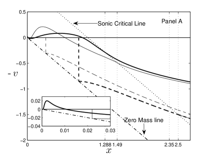
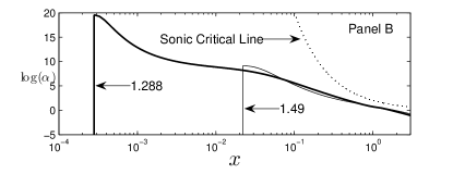
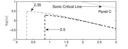
Figure 3: Four typical type $\mathcal{X}_{\rm II}$ ISSV solutions in $-v(x)$ versus $x$ profile. Values of their $x_{*}$ are marked by the grid lines of $x-$axis in panel A. The inner box presents details of two curves near $x\rightarrow 0^{+}$ in the same line type as corresponding curves in Panel A. Panel B and C give the four solutions in $\log\alpha$ versus $x$ profile. Panel B presents two solution curves of II’ condition marked with $x_{*}=1.288$ (heavy solid line) and $x_{*}=1.49$ (light solid line) respectively and panel C shows two solution curves of IV’ condition marked with $x_{*}=2.35$ (light dash line) and $x_{*}=2.5$ (heavy dash line) respectively. The density jumps at $x_{0}$ are obviously much sharper in condition II’ than in condition IV’ (compare the numbers along $y-$axes).

Table 3: Parameters of several typical type $\mathcal{X}_{\rm II}$ ISSV solutions. Five solutions under two conditions in Section 3.3.1 are listed below.

  Condition $x_{*}$ $x_{0}$ $\alpha_{0}$ $V$ $A$ II’ $1.288$ $2.8\times 10^{-4}$ $4\times 10^{8}$ $1.5$ $4.7$ II’ $1.49$ $0.022$ $9.1\times 10^{3}$ $4.5$ $18$ IV’ $2.35$ $0.304$ $1.61$ $3.30$ $8.54$ IV’ $2.5$ $0.852$ $1.32$ $3.46$ $8.92$ IV’ $2.58$ $1.007$ $1.23$ $9.48$ $3.54$  

3.3.3 Interpretations for Type $\mathcal{X}$ ISSV Solutions

We have explored all possible type $\mathcal{X}$ ISSV solutions. Now we offer interpretations for these solutions. In preceding sections, we used parameter $x_{*}$ on the SCL as the key parameter to construct type $\mathcal{X}$ ISSV solutions. This method assures us not to miss any possible ISSV solutions. However, for ISSV solutions, $x_{0}$ and $\alpha_{0}$ are the most direct parameters describing properties of central void expansions.

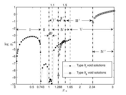
Figure 4: The relation between isothermal void boundary $x_{0}$ and the sonic point $x_{*}$ at SCL. The ‘solid circle curve’ and the ‘open circle curve’ are the $\log(x_{0})$ versus $x_{*}$ curves of type $\mathcal{X}_{\rm I}$ and type $\mathcal{X}_{\rm II}$ void solutions. The key numerals dividing the positive real $x-$axis into several ranges are indicated by the dash vertical lines with numerals marked along or at $x-$axis. In regions I, II, III, and IV, we have four branches for type $\mathcal{X}_{\rm I}$ void solutions. In regions II’ and IV’, we have two branches for type $\mathcal{X}_{\rm II}$ ISSV solutions.

The void edge $x_{0}$ is the reduced radius in the self-similar description and $ax_{0}$ is the expansion speed of the void boundary. We adjust the $x_{*}$ value at the SCL to search for void solutions and there exists a certain relationship between $x_{*}$ and $x_{0}$ as expected. Figure 4 shows these relationships for types $\mathcal{X}_{\rm I}$ and $\mathcal{X}_{\rm II}$ ISSV solutions.

Under conditions I, II, III and given $x_{*}$, the corresponding $x_{0}$ runs from $0$ to a maximum value and then back to $0$. The maximum values of conditions I, II and III are $x_{0}=0.042$, $x_{0}=8\times 10^{-4}$ and $x_{0}=0.9\times 10^{-4}$ which correspond to $x_{*}\approx 0.5$, $x_{*}\approx 0.89$ and $x_{*}\approx 1.04$, respectivly. For $x_{*}$ under conditions IV or II’, the corresponding $x_{0}$ increases with $x_{*}$ and the intervals of $x_{0}$ are $[0^{+},0.027]$ and $[0^{+},0.022]$, respectively. Under condition IV’, $x_{0}$ increases with $x_{*}$ from $[0^{+},+\infty)$ monotonically. However, when $x_{*}$ is under condition IV’, the corresponding $x_{0}$ is usually very large (at least 100 times larger) compared to other type $\mathcal{X}$ ISSV solutions unless $x_{*}$ is near $2.34$. Physically under condition IV’, isothermal voids usually expand at a relatively high speed. Based on the value and meaning of $x_{0}$, type $\mathcal{X}$ ISSV solutions can be divided into two classes: rapid and slow ISSV expansion solutions. All type $\mathcal{X}_{\rm I}$ ISSV solutions and type $\mathcal{X}_{\rm II}$ ISSV solutions under condition II’ belong to slow void expansion solutions. Type $\mathcal{X}_{\rm II}$ ISSV solutions under condition IV’ belong to rapid void expansion solutions.

Parameter $\alpha_{0}$ represents the reduced density $\alpha$ at the void boundary. Figures 2 and 3 and Tables 2 and 3 clearly indicate that isothermal voids, described by type $\mathcal{X}$ ISSV solutions, are all surrounded by dense mass shells and the gas density around voids attenuates monotonically with increasing radius. So there are classes of voids that evolve with fairly sharp edges but without shocks. Nevertheless, sharp edge around voids is not a general property of all void solutions. Expanding voids with shocks can be surrounded by quasi-smooth edges (never smooth edges as shown in Appendix A). In Section 4, we will show that $\alpha_{0}$ is an important parameter which may reveal the mechanism that generates and sustains a void. Large $\alpha_{0}$ requires very energetic mechanisms against the high inward pressure across the boundary. So type $\mathcal{X}$ voids may be difficult to form because all type $\mathcal{X}$ voids have dense boundaries.

Figures 2 and 3 and Tables 2 and 3 clearly show that all type $\mathcal{X}_{\rm II}$ void solutions and type $\mathcal{X}_{\rm I}$ ISSV solutions under conditions III and IV describe isothermal voids surrounded by gas envelopes in expansion (i.e. velocity parameter $V$ at $x\rightarrow\infty$ are positive). Astrophysical void phenomena are usually coupled with outflows (i.e. winds). Our ISSV solutions indicate that rapidly expanding voids must be surrounded by outflows.

Type $\mathcal{X}_{\rm I}$ ISSV solutions under conditions I and II describe voids surrounded by contracting envelopes, although under these two conditions the voids expand very slowly ($\leq 0.042a$, see subsection 3.3.1) and are surrounded by very dense shells (see Table 2).

Outflows and inflows are possible as indicated by type $\mathcal{X}$ ISSV solutions, but no static shell is found in type $\mathcal{X}$ ISSV solutions. In the following section, we show voids with shocks being surrounded by static envelopes.

A clarification deems appropriate here that division of the $x>0$ axis in subsection 3.3.1 is actually not precise. In subsection 3.3.1, we divide $(0,+\infty)$ into six intervals by five points $x_{1}$ to $x_{5}$ and $x_{1}$, $x_{3}$ and $x_{4}$ are the cross points at the SCL of Lou & Shen type2-type1 solution. We note that they are only the first three examples of an infinite number of discrete solutions that cross the SCL smoothly twice via type 2 derivative first at a smaller $x$ and then type 1 derivative at a larger $x$ (Lou & Shen 2004). Our numerical computations show that the fourth type2-type1 solution will pass the SCL smoothly at $x_{*}(1)\approx 4\times 10^{-8}$ and $x_{*}(2)=0.97$, so there should be another regime of $0.97<x<1=x_{2}$ inside condition II. The first four right cross points of type2-type1 solutions are $1.65$, $0.743$, $1.1$ and $0.97$. By inference, the cross points of the fifth and following type2-type1 solutions will be narrowly located around $x=1$. When the infinite number of type2-type1 solutions are taken into account, there will be fine structures around $x=1$ in subsection 3.3.1 and Figure 4. However, the solution behaviours of crossing the SCL smoothly under condition of fine structure are like those under conditions II, III and IV near $x=1$.

3.4 Type $\mathcal{Z}$ Voids: ISSV Solutions with Shocks

Shock phenomena are common in various astrophysical flows, such as planetary nebulae, supernova remnants, and even galaxy clusters gas (e.g. Castor et al. 1975; McNamara et al. 2005). In this subsection, we present type $\mathcal{Z}$ ISSV solutions, namely, self-similar void solutions with shocks. Equations (16) and (17) are mass and momentum conservations. The isothermality is a strong energy requirement. In our isothermal model, an example of polytropic process, the energy process is simplified. This simplification gives qualitative or semi-quantitative description of the energy process for a shock wave. By introducing parameter $\tau$ for the temperature difference after and before a shock, we can describe more classes of shocks (Bian & Lou 2005).

The basic procedure to construct a spherical ISSV solution with shocks is as follows. Given $(x_{0},\ v_{0}=x_{0},\ \alpha_{0})$ at the void boundary, we can integrate ODEs (8) and (9) outwards from $x_{0}$; in general, numerical solutions cannot pass through the SCL smoothly (if they do, they will be referred to as type $\mathcal{X}$ ISSV solutions); however, with an outgoing shock, solutions can readily cross the SCL (e.g. Tsai & Hsu 1995; Shu et al. 2002; Shen & Lou 2004; Bian & Lou 2005); finally global ($x_{0}<x<+\infty$) solutions can be constructed by a combination of integration from $x_{0}$ to $x_{ds}$, shock jump and integration from $x_{us}$ to $+\infty$, where $x_{ds}$ and $x_{us}$ are defined in subsection 2.2 as the radial expanding velocity of a shock on the downstream and upstream sides, respectively.

A typical ISSV solution with a shock has four degrees of freedom (DOF) within a sensible parameter regime. For example, we need independent input of $x_{0}$, $\alpha_{0}$, $x_{ds}$ and $\tau$ to determine an ISSV solution with a shock, while the degree of freedom for type $\mathcal{X}$ solutions is one (i.e. $x_{*}$ plus the type of eigen-derivative crossing the SCL are enough to make a type $\mathcal{X}$ ISSV solution). When we consider the simplest condition that $\tau=1$, the DOF of a void solution with shocks is three. So infinite void shock solutions exist. By fixing one or two parameters, we can enumerate all possible values of the other parameter to obtain all possible ISSV solutions. For example, by fixing velocity parameter $V$, we can adjust mass parameter $A$ and $x_{us}$ to explore all void solutions (see equation 15); following this procedure, $x_{0}$, $\alpha_{0}$ and $x_{ds}$ are determined by $V$, $A$ and $x_{us}$. There is a considerable freedom to set up an ISSV solution with shocks. In astrophysical flows, we would like to learn the expansion speed of a void, the density surrounding a void and the radial speed of gas shell at large radii. We then choose one or two parameters in $x_{0}$, $\alpha_{0}$ and $V$ as given parameters to search for ISSV solutions by changing other parameters such as $x_{us}$.

In Section 3.4.1, we will first consider the simple case: equi-temperature shock void (i.e. $\tau=1$), and refer to as void solutions with equi-temperature shocks or type $\mathcal{Z}_{\rm I}$ ISSV solutions. Several type $\mathcal{Z}_{\rm I}$ voids with different behaviours near void boundaries and outer envelopes (a static envelope, outflows and inflows) will be presented. Phase diagram matching method will be described and extended to the so-called ‘phase net’, with the visual convenience to search for ISSV solutions with more DOF. Section 3.4.2 presents type $\mathcal{Z}_{\rm II}$ ISSV solutions: void solutions with two-soundspeed shocks (i.e. $\tau>1$).

3.4.1 Type $\mathcal{Z}_{\rm I}$ Void Solutions: Voids
    with Same-Soundspeed Shocks

For an equi-temperature shock, we have $\tau=1$ and thus $x_{ds}=x_{us}=x_{s}$ (see Section 2.2). As already noted, the DOF of $\mathcal{Z}_{\rm I}$ void solutions is three. We can use $\{x_{0},\ \alpha_{0}$, $\ x_{s}\}$ to construct type $\mathcal{Z}_{\rm I}$ ISSV solutions.

We have freedom to set the condition $(x_{0},\ \alpha_{0})$ at the void edge to integrate outwards. Before reaching the SCL, we set an equi-temperature shock at a fairly arbitrary $x_{s}$ to cross the SCL. We then combine the integrations from $x_{0}$ to $x_{s}^{-}$ and from $x_{s}^{+}$ to $+\infty$ by a shock jump to form a type $\mathcal{Z}_{\rm I}$ ISSV solution with a shock.

We emphasize that under type $\mathcal{Z}_{\rm I}$ condition, the insertion of an equi-temperature shock does assure that void solutions jump across the SCL. Physics requires that at every point $(x,\ v(x),\ \alpha(x))$ of any void solution, there must be $x>v(x)$ for a positive mass. Equation (21) indicates that across the equi-temperature shock front, the product of two negative $v_{d}-x_{s}$ and $v_{u}-x_{s}$ makes 1. In our model, $x_{s}-v_{d}<1$ so $x_{s}-v_{u}$ must be larger than $1$. So the downstream and upstream are separated by the SCL. However, in type $\mathcal{Z}_{\rm II}$ condition with $\tau>1$, this special property may not always hold on. We shall require such a separation across the SCL as a necessary physical condition.

Figure 5 shows several type $\mathcal{Z}_{\rm I}$ ISSV shock solutions with void expansion at half sound speed and $0.03$ times sound speed. From this figure, we know that even the voids expand at the same speed, with different density $\alpha_{0}$ near the void edge and the radial velocities of the shock wave ($x_{s}$), they can have outer envelopes of various dynamic behaviours. From values of $v(x)$ and $\alpha(x)$ at large $x$ (say 10), we can estimate $V$ and $A$. Different from type $\mathcal{X}$ ISSV solutions, some type $\mathcal{Z}_{\rm I}$ ISSV shock solutions have outer envelopes with a negative $V$ (e.g. curves $1^{\prime}$ and $2^{\prime}$ in Fig. 5), that is, contracting outer envelopes. Numerical calculations show that voids with contracting envelopes usually expand very slowly (voids $1^{\prime}$ and $2^{\prime}$ in Fig. 5 expand at $0.03a$).

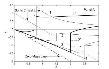
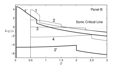
Figure 5: We show six type $\mathcal{Z}_{\rm I}$ void shock solutions. Four of them have same $x_{0}=0.5$ but different values of $\alpha_{0}$ marked by numbers $1,2,3,4$. The other two have same $x_{0}=0.03$ but different values of $\alpha_{0}$ marked by number $1^{\prime},2^{\prime},3^{\prime},4^{\prime}$. Panel A above presents $-v(x)$ versus $x$ profiles and panel B below shows $\log\alpha$ versus $x$ profiles. Values of the two free parameters $(\alpha_{0},\ x_{s})$ are $(50,\ 0.8)$, $(5,\ 1.5)$, $(1,\ 2.3)$, $(0.1,\ 2.5)$ for curves $1,2,3,4$, respectively; and $(100,\ 0.7)$, $(0.01,\ 2)$ for curves $1^{\prime}$ and $2^{\prime}$, respectively. The dotted curves in both panels are Sonic Critical Line.

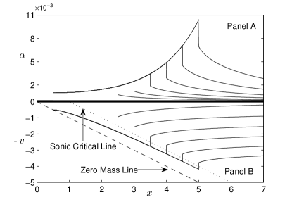
Figure 6: Several type $\mathcal{Z}_{I}$ ISSV solutions with quasi-smooth edges in light solid curves with the same values of $x_{0}=0.5$ and $\alpha_{0}=10^{-3}$ but different shock speed $x_{s}$ from $2.5$ to $5.0$ every $0.5$ in step. Panel A presents $\alpha(x)$ versus $x$ profiles and panel B shows $-v(x)$ versus $x$ profiles. The dotted and dash lines in panel B are the SCL and the ZML, respectively.

In addition to shocks and outer envelope dynamics, another important difference between type $\mathcal{Z}_{I}$ and type $\mathcal{X}$ ISSV solutions lies in behaviours of shells surrounding the void edge. From Section 3.3 (see Fig. 2), we have known that the reduced mass density of type $\mathcal{X}$ void solutions must encounter a sharp jump and decrease monotonically with increasing $x$. However, Fig. 5 (curves $4$ and $2^{\prime}$ with the y-axis in logarithmic scales) and Fig. 6 indicate that with shocks involved, the density of shells near void edges can increase with increasing $x$. Under these conditions, density jumps from a void to gas materials around voids appear not to be very sharp. Voids described by solutions like curves in Figure 6 and curves $4$ and $2^{\prime}$ in Figure 5 have such ‘quasi-smooth’ edges. These solutions can approximately describe a void with a smooth edge, whose outer shell gradually changes from vacuum in the void to gas materials, without sharp density jump. Or, they describe a void with a quasi-smooth edge, whose outer shell gradually changes from vacuum in the void to gas materials, with a small density jump. Figure 6 clearly shows that the faster a shock moves relative to void edge expansion, the higher density rises from void edge to shock.

Type $\mathcal{Z}_{\rm I}$ Voids with a SIS Envelope

Void phenomena in astrophysics indicate an expanding void in the centre and static gas medium around it in the outer space. For example, a supernova explodes and ejects almost all its matter into space. If the shock explosion approximately starts from the central core of the progenitor star, the remnant of the supernova is then approximately spherically symmetric and a void may be generated around the explosion centre (e.g. Lou & Cao 2008). If the gravity of the central compact object may be ignored, we then describe this phenomenon as an expanding spherical void surrounded by a static outer envelope. The analysis of Section 3.3.3 indicates that all type $\mathcal{X}$ ISSV solutions cannot describe this kind of phenomena. However with rebound shocks, it is possible to construct a model for an expanding void surrounded by a static SIS envelope.

Shu (1977) constructed the expansion-wave collapse solution (EWCS) to describe a static spherical gas with an expanding region collapsing towards the centre. In fact, EWCS outer envelope with $x>1$ is the outer part of a SIS solution (see equation 11). We now construct several ISSV solutions with an outer SIS envelope. An outer SIS envelope has fixed two DOF of a type $\mathcal{Z}_{\rm I}$ ISSV solution, that is, $V=0$ and $A=2$, so there is only one DOF left. A simple method is to introduce a shock at a chosen point $x_{s}$ of EWCS solution except $(x=1,\ v=0,\ \alpha=1)$ (we emphasize that only one point $(x=1,\ v=0,\ \alpha=1)$ of the EWCS solution is at the SCL and all the other points lay on the upper right to the SCL in the $-v(x)$ versus $x$ profile) and make the right part of EWCS solution the upstream of a shock, then we can obtain $(v_{ds},\ \alpha_{ds})$ on the downstream side of a shock. If the integration from $(x_{s},\ v_{ds},\ \alpha_{ds})$ leftward touches the ZML at $x_{0}$, a type $\mathcal{Z}_{\rm I}$ ISSV solution with a static outer envelope is then constructed.

We introduce the $\alpha-v$ phase diagram to deal with the relationship among the free parameters and search for eigensolutions of ODEs (8) and (9). Hunter (1977) introduced this method to search for complete self-similar eigensolutions of two ODEs. Whitworth & Summer (1985) used this method to combine free-fall solutions and LP solutions in the centre with certain asymptotic solutions at large radii. Lou & Shen (2004) applies this method to search for eigensolutions of ODEs (8) and (9) which can cross the SCL twice smoothly. In the case of Lou & Shen (2004), the DOF is 0. So there is an infinite number of discrete eigensolutions.

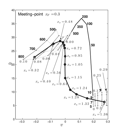
Figure 7: The phase diagram of $\alpha$ versus $v$ at a chosen meeting point $x_{F}=0.3$ for match of the SIS solution (e.g., Shu 1977) and type $\mathcal{Z}$ void shock solutions. Each open circle symbol joint by a heavy solid curve denotes an integration from a chosen $x_{s}$ (marked besides each open circle) towards $x_{F}<x_{s}$. We impose the equi-temperature shock conditions at $x_{s}$ from $0.32$ to $1.36$ for the outer SIS solution and then integrate from $x_{s}$ back to $x_{F}$ to get $[v(x_{F}),\ \alpha(x_{F})]$ as marked in the phase diagram. The change of $x_{s}$ naturally leads to a phase curve shown here by the heavy solid curve. We choose the range of $x_{s}$ to be $[0.32,\ 1.36]$ because $x_{s}$ must be larger than $x_{F}$ and a larger $x_{s}$ than $1.36$ will give rise to solution curves encountering the SCL at $x\geq x_{F}=0.3$. Meanwhile, two “phase nets”, made of the light solid curves and dotted curves and connected by a medium heavy solid curve, are actually generated by integrations from chosen $(x_{0},\ v_{0}=x_{0},\ \alpha_{0})$. Each solid curve in the two nets (including the connecting medium heavy solid curve) is an equal$-x_{0}$ curve, that is, every point in the same solid curve corresponds to the same value of $x_{0}$ noted besides each equal$-x_{0}$ curve; and each dotted curve in the two nets is an equal$-\alpha_{0}$ curve with the value of $\alpha_{0}$ in boldface noted besides each curve. For the lower right net, the points in the net correspond to an initial condition of $(x_{0},\ \alpha_{0})\in\{x_{0}|x_{0}\in[0,0.29]\}\times\{\alpha_{0}|\alpha_{0}\in[5,10]\}$; the value of $x_{0}$ is $0$, $0.15$, $0.2$, $0.25$, $0.29$ respectively from the left equal-$x_{0}$ solid curve to the right one and the value of $\alpha_{0}$ is $5$, $7$, $9$, $10$ respectively from the bottom equal-$\alpha_{0}$ dotted curve to the top one. For the upper left net, the points in the net correspond to an initial condition of $(x_{0},\ \alpha_{0})\in\{x_{0}|x_{0}\in[0,0.1]\}\times\{\alpha_{0}|\alpha_{0}\in[500,800]\}$; the value of $x_{0}$ is $0$, $0.04$, $0.06$, $0.08$, $0.10$ respectively from the right equal-$x_{0}$ solid curve to the left one and the value of $\alpha_{0}$ is $500$, $600$, $700$, $800$ respectively from the top equal-$\alpha_{0}$ dotted curve to the bottom one. The medium solid curve is an equal-$x_{0}$, too, with $x_{0}=0$ and $\alpha_{0}=10$, $50$, $100$, $200$, $350$ and $500$ from lower right to left. This medium solid curve shows the trend of phase curves as we increase $\alpha_{0}$ value in large steps.

For type $\mathcal{Z}_{\rm I}$ ISSV shock solutions with a static SIS outer envelope, the DOF is one. We insert a shock at $x_{s}$ in the SIS and then integrate inwards from $x_{s}$ to a fixed meeting point $x_{F}$. Adjusting the value of $x_{s}$ will lead to a phase curve $[v(x_{F})^{+},\ \alpha(x_{F})^{+}]$ in $\alpha$ versus $v$ phase diagram. Meanwhile, an outward integration from a chosen void boundary condition $(x_{0},\ v_{0}=x_{0},\ \alpha_{0})$ reaches a phase point $[v(x_{F})^{-},\ \alpha(x_{F})^{-}]$ at $x_{F}$. Varying values of $x_{0}$ or $\alpha_{0}$ will lead to another phase curve $[v(x_{F})^{-},\ \alpha(x_{F})^{-}]$ in the $\alpha$ versus $v$ phase diagram. We note that changing both values of $x_{0}$ and $\alpha_{0}$ will result in a “phase net” (i.e. a two-dimensional mesh of phase curves) in $\alpha$ versus $v$ diagram (see Fig. 7). If such a “phase net” of $(x_{0},\ \alpha_{0})$ and the phase curve of $x_{s}$ share common points (usually, there will be an infinite number of common points continuously as such “phase net” is two dimensional), type $\mathcal{Z}_{\rm I}$ ISSV shock solutions with a static SIS envelope can be constructed.

Figure 7 presents the phase diagram at a meeting point $x_{F}=0.3$ to search for type $\mathcal{Z}_{\rm I}$ ISSV shock solutions with an outer SIS envelope. Note that part of the phase curve falls into the phase net, revealing that an infinite number of type $\mathcal{Z}_{\rm I}$ ISSV shock solutions with outer SIS envelope indeed exist continuously. Shown by Figure 7, numerical results suggest that when shock position $x_{s}>0$ is less than $0.62$ or larger than $1.335$, there is at least one type $\mathcal{Z}_{\rm I}$ ISSV that can exist in the downstream side of a shock. However, if a shock expands at a radial velocity between $0.62a$ and $1.335a$, it is impossible for a type $\mathcal{Z}_{\rm I}$ ISSV to exist inside a shock with a SIS envelope. Table 4 contains values of $x_{0}$, $\alpha_{0}$ and $x_{s}$ of some typical type $\mathcal{Z}_{\rm I}$ ISSV shock solutions with a SIS envelope. Figure 8 is a phase diagram showing how $x_{0}$ and $\alpha_{0}$ are evaluated with $x_{s}$ changing to construct a type $\mathcal{Z}_{\rm I}$ ISSV shock solutions with an outer SIS envelope.

Table 4: Values of $x_{0}$, $\alpha_{0}$ and $x_{s}$ for several type $\mathcal{Z}_{\rm I}$ void shock solutions with an outer static SIS envelope are summarized here

  $x_{0}$ $\alpha_{0}$ $x_{s}$ $0.018$ $4.3\times 10^{6}$ $0.02$ $0.063$ $1.5\times 10^{4}$ $0.1$ $0.09$ $1.1\times 10^{3}$ $0.26$ $0.077$ $5.9\times 10^{2}$ $0.4$ $0.01$ $9.5\times 10^{2}$ $0.62$ $<0.005$ $7.9$ $1.335$ $0.12$ $7.5$ $1.338$ $0.27$ $6.3$ $1.36$ $0.65$ $4.1$ $1.5$ $2.65$ $2.3$ $3.00$  

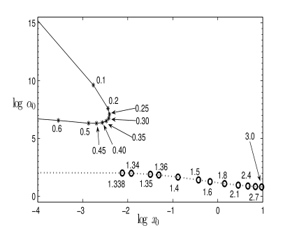
Figure 8: The phase diagram of $\log\alpha_{0}$ versus $\log x_{0}$ shows the relationship among $x_{s}$, $x_{0}$ and $\alpha_{0}$ of type $\mathcal{Z}_{\rm I}$ void shock solutions with a static SIS envelope. The DOF of these three parameters is only one; i.e. given arbitrary one of the three, the other two parameters are determined in constructing a type $\mathcal{Z}_{\rm I}$ void shock solutions with a static SIS envelope. For any point in the two curves, $x_{0}$ and $\alpha_{0}$ indicated by its $x$ and $y$ coordinates with $x_{s}$ marked, correspond to a type $\mathcal{Z}_{\rm I}$ void shock solution. The upper left solid curve with its data points in asterisk symbol corresponds to the condition $x_{s}<0.62$ and the lower dotted curve with its data points in open circle corresponds to the condition $x_{s}>1.335$. The first condition referred to as Class I gives its largest $x_{0}=0.09$ when $x_{s}=0.26$. Although $x_{0}$ for the second condition referred to as Class II ranges along the entire real axis, it usually takes a relative large value; moreover, in Class II solutions, the reduced density $\alpha_{0}$ at the void boundary is in the order of unity.

All of Fig. 7, Fig. 8 and Table 4 clearly indicate type $\mathcal{Z}_{\rm I}$ ISSV shock solutions with a SIS envelope can be generally divided into two classes according to $x_{s}$. Class I type $\mathcal{Z}_{\rm I}$ void shock solutions with an outer static SIS envelope have $x_{s}<0.62$ usually with a smaller value of $x_{0}$ and a higher value of $\alpha_{0}$. Class II solutions have $x_{s}>1.335$ usually with a larger value of $x_{0}$ and a medium value of $\alpha_{0}$. By a numerical exploration, the maximum of $x_{0}$ of Class I solutions is $\sim 0.09$ for $x_{s}=0.26$ and $\alpha_{0}=1.1\times 10^{3}$; these voids expand at a low speed of $<0.1a$; and the reduced density $\alpha_{0}$ at the void boundary is usually $>10^{2}$, indicating a sharp edge density peak. Finally, we note that Class I voids involve shocks expanding at subsonic speeds. In this situation, the outer region $x>x_{s}$ is not completely static. The SIS envelope only exists at $x\geq 1$, and the region between $x_{s}$ and $1$ is a collapse region (see two class I ISSV shock solutions 1 and 2 in Fig. 9). While in Class II ISSV shock solutions, shock expands supersonically and with $x_{0}$ usually relatively large. So the upstream side of a shock in Class II ISSV solutions is static (see two class II ISSV solutions 3 and 4 shown in Fig. 9). In rare situations, $x_{0}$ can be small (e.g. $x_{s}<1.4$) and $\alpha_{0}$ neither large nor small, indicating that Class II voids have moderately sharp edges.

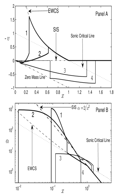
Figure 9: Four typical type $\mathcal{Z}_{\rm I}$ void shock solutions with static SIS envelope. The two heavy solid curves in both panels are the Class I type $\mathcal{Z}_{\rm I}$ void solutions with a SIS envelope and a subsonic shock (i.e., $x_{s}<1$), and the two light solid curves in both panels are the Class II type $\mathcal{Z}_{\rm I}$ void solutions with an outer SIS envelope and a supersonic shock (i.e., $x_{s}>1$). Panel A presents $-v(x)$ versus $x$ profiles. Panel B presents $\alpha$ versus $x$ profiles using a logarithmic scale along the $y-$axis. The key data $(x_{0},\ \alpha_{0},\ x_{s})$ of these solutions are $(0.09,\ 1.1\times 10^{3},\ 0.26)$, $(0.01,\ 9.5\times 10^{2},\ 0.62)$, $(0.12,\ 7.5,\ 1.338)$, and $(0.65,\ 4.1,\ 1.50)$ for curves 1, 2, 3, and 4, respectively. The dash curves in both panels are part of the EWCS solution.

Type $\mathcal{Z}_{\rm I}$ voids with expanding envelopes: breezes, winds, and outflows

In our ISSV model, we use parameters $V$ and $A$ to characterize dynamic behaviours of envelopes. Equation (15) indicates that $V>0$ describes an expanding envelope at a finite velocity of $Va$, and a larger $A$ corresponds to a denser envelope. For $V=0$, the expansion velocity vanishes at large radii, corresponding to a breeze; a smaller $A$ than $2$ is required to make sure an outer envelope in breeze expansion. For $V>0$, the outer envelope is a wind with finite velocity at large radii.

We apply the similar method to construct type $\mathcal{Z}_{\rm I}$ voids with expanding envelopes as we deal with type $\mathcal{Z}_{\rm I}$ voids with outer SIS envelopes. The difference between the two cases is that $V$ and $A$ are allowed to be different from $V=0$ and $A=2$. In this subsection, we usually choose a meeting point $x_{F}$ between $x_{0}$ and $x_{s}$. Then by varying $x_{0}$ and $\alpha_{0}$, we obtain a phase net composed by $[v(x_{F})^{-},\ \alpha(x_{F})^{-}]$. Given $V$, we adopt $A$ and integrate ODEs (8) and (9) from large $x$ towards $x_{s}$. After setting a shock at $x_{s}$, we integrate ODEs towards $x_{F}$. By varying $A$ and $x_{s}$, we obtain a phase net composed by $[v(x_{F})^{+},\ \alpha(x_{F})^{+}]$. The overlapped area of two phase nets reveals the existence of type $\mathcal{Z}_{\rm I}$ ISSV with dynamic envelopes characterized by $V$ and $A$.

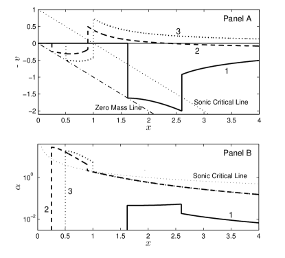
Figure 10: Three typical type $\mathcal{Z}_{\rm I}$ void shock solutions with different outer envelopes. Panel A presents $-v(x)$ versus $x$ profiles. Panel B presents $\alpha(x)$ versus $x$ profiles in a logarithmic scale along the $y-$axis. The heavy solid curve $1$ gives a type $\mathcal{Z}_{\rm I}$ void shock solution with a quite thin breeze outer envelope whose $(x_{0},\ \alpha_{0},\ x_{s},\ V,\ A)=(1.62,\ 0.046,\ 2.6,\ 0,\ 0.1)$. The heavy dash curve $2$ gives a type $\mathcal{Z}_{\rm I}$ void shock solution with a wind outer envelope whose $(x_{0},\ \alpha_{0},\ x_{s},\ V,\ A)=(0.25,\ 28.2,\ 0.90,\ 0.2,\ 2.5)$. The heavy dotted curve $3$ gives a type $\mathcal{Z}_{\rm I}$ void shock solution with an accretion outer envelope whose $(x_{0},\ \alpha_{0},\ x_{s},\ V,\ A)=(0.50,\ 18.8,\ 1.00,\ 0,\ 2.50)$. The monotonic dotted curves in both panels stand for the SCL.

Figure 10 gives two examples of type $\mathcal{Z}_{\rm I}$ voids with breeze and wind. We emphasize that $A>2$ is required in such ISSV solutions with an outer envelope wind and subsonic shock. Actually, the larger the velocity parameter $V$ is, the smaller the mass parameter $A$ is needed. Large $A$ is required to guarantee that the upstream region of a global solution is on the upper right part of the SCL when the shock moves subsonically (i.e. $x_{s}<1$). Physically, if an ISSV is surrounded by a subsonic shock wave, the wind outside needs to be dense enough.

Type $\mathcal{Z}_{\rm I}$ voids with contracting outer envelopes: accretions and inflows

We explore ISSV with contracting envelopes, such as accretion envelopes. Type $\mathcal{X}_{\rm I}$ voids under conditions I and II have contracting envelopes. These type $\mathcal{X}_{\rm I}$ voids are all surrounded by very dense shells with density decreasing with increasing radius. With shocks involved, central voids can have envelopes of various properties. Type $\mathcal{Z}_{\rm I}$ voids with contracting outer envelopes are also studied. To have a contracting envelope, the velocity parameter $V$ should be negative or approach $0^{-}$. A negative $V$ and a positive $A$ describe an outer envelope inflowing at a velocity of $aV$ from large radii. For $V=0$ and $A>2$, an outer envelope has an inflow velocity vanishing at large radii (Lou & Shen 2004; Bian & Lou 2005). Figure 10 gives examples of type $\mathcal{Z}_{\rm I}$ voids with accreting outer envelopes.

3.4.2 Type $\mathcal{Z}_{\rm II}$ ISSV Solutions: Voids Surrounded by Two-Soundspeed Shocks in Envelopes

In the previous section, we explored type $\mathcal{Z}_{\rm I}$ ISSV solutions featuring the equi-temperature shock. There, $\tau=1$ indicates the same sound speed $a$ across a shock. The isothermal sound speed $a$ can be expressed as

$$a=\left(\frac{p}{\rho}\right)^{1/2}=\left[\frac{(Z+1)k_{B}}{\mu}T\right]^{1/2}\ ,$$ (23)

where $k_{B}$ is Boltzmann’s constant, $\mu$ is the mean atomic mass and $Z$ is the ionization state. $Z=0$ corresponds to a neutral gas and $Z=1$ corresponds to a fully ionized gas. In various astrophysical processes, shock waves increase the downstream temperature, or change the proportion of gas particles; moreover, the ionization state may change after a shock passage (e.g. champagne flows in H_II regions, Tsai & Hsu 1995; Shu et al. 2002; Bian & Lou 2005; Hu & Lou 2008). Such processes lead to two-soundspeed shock waves with $\tau>1$. In this section, we consider $\tau>1$ for type $\mathcal{Z}_{\rm II}$ ISSV shock solutions with two-soundspeed shocks. Global $\mathcal{Z}_{\rm II}$ void solutions have temperature changes across shock waves while both downstream and upstream sides remain isothermal, separately. With a range of $\tau>1$, it is possible to fit our model to various astrophysical flows.

For $\tau>1$, the DOF of type $\mathcal{Z}_{\rm II}$ ISSV shock solutions is four, i.e. one more than that of type $\mathcal{Z}_{\rm I}$ ISSV shock solutions with $\tau=1$. We will not present details to construct type $\mathcal{Z}_{\rm II}$ ISSV shock solutions as they differ from the corresponding type $\mathcal{Z}_{\rm I}$ ISSV shock solution only in the quantitative sense. General properties such as the behaviours near the void boundary and the outer envelope of type $\mathcal{Z}_{\rm II}$ ISSV shock solutions remain similar to those of type $\mathcal{Z}_{\rm I}$ ISSV shock solutions. We present examples of typical type $\mathcal{Z}_{\rm II}$ ISSV shock solutions in Figure 11.

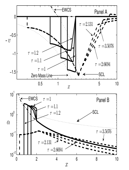
Figure 11: Six type $\mathcal{Z}$ ISSV solutions with shocks. Panel A presents $-v(x)$ versus $x$ profiles and panel B presents $\alpha(x)$ versus $x$ profiles. The heavy solid curves labelled by their corresponding $\tau$ in both panels are type $\mathcal{Z}$ ISSV shock solutions with $x_{s}=2$ and $\tau=1,\ 1.1,\ 1.2$ respectively. The $\tau=1$ case is a type $\mathcal{Z}_{\rm I}$ ISSV shock solution and the latter two with $\tau>1$ are type $\mathcal{Z}_{\rm II}$ ISSV shock solutions. The heavy dash curves labelled by their corresponding $\tau$ in both panels are solutions with reduced velocity $V=0$ and $A=1,\ 1.5,\ 2.5$ respectively. The one with $A=2.5$ has an envelope accretion and the other two have envelope breezes. The relevant data of these six solutions are summarized in Table 5. Shock jumps of type $\mathcal{Z}_{\rm II}$ ISSV solutions do not appear vertical as those of type $\mathcal{Z}_{\rm I}$ ISSV shock solutions (e.g. Bian & Lou 2005) because of different sound speeds across a shock front and thus different scales of reduced radial $x\equiv r/(at)$.

Table 5: Parameters of several type $\mathcal{Z}_{\rm I}$ and $\mathcal{Z}_{\rm II}$ ISSV shock solutions shown in Figure 11

  $x_{0}$ $\alpha_{0}$ $x_{ds}$ $x_{us}$ $\tau$ $V$ $A$ $1.45$ $2.72$ $2$ $2$ $1$ $0$ $2$ $1.12$ $2.81$ $1.82$ $2$ $1.1$ $0$ $2$ $0.74$ $3.51$ $1.67$ $2$ $1.2$ $0$ $2$ $2.65$ $2.26$ $3$ $3$ $1$ $0$ $2$ $1.21$ $1.87$ $2$ $3$ $1.5$ $0$ $2$ $0.3$ $0.1$ $2.2303$ $4.7528$ $2.131$ $0$ $1$ $0.3$ $0.1$ $2.2064$ $5.8898$ $2.6694$ $0$ $1.5$ $0.3$ $0.1$ $2.1886$ $7.6767$ $3.5076$ $0$ $2.5$  

4 Astrophysical Applications

4.1 The role of self-gravity in gas clouds

Earlier papers attempted to build models for hot bubbles and planetary nebulae (e.g. Weaver et al. 1977; Chevalier 1997a) without including the gas self-gravity. In reference to Chevalier (1997a) and without gravity, our nonlinear ODEs (8) and (9) would then become

$$\left[(x-v)^{2}-1\right]\frac{dv}{dx}=-\frac{2}{x}(x-v)\ ,$$ (24)

$$\left[(x-v)^{2}-1\right]\frac{1}{\alpha}\frac{d\alpha}{dx}=-\frac{2}{x}(x-v)^{2}\ .$$ (25)

ODEs (24) and (25) allow both outgoing and inflowing outer envelopes around expanding voids. Self-similar solutions of ODEs (24) and (25) cannot be matched via shocks with a static solution of uniform mass density $\rho$. For comparison, the inclusion of self-gravity can lead to a static SIS. In some circumstances, there may be no apparent problem when ODEs (24) and (25) are applied to describe planetary nebulae because AGB wind outer envelope may have finite velocity at large radii. However, in the interstellar bubbles condition, a static ISM should exist outside the interaction region between stellar wind and ISM. In Weaver et al. (1977), a static uniformly distributed ISM surrounding the central bubble was specifically considered. In our ISSV model, a single solution with shock is able to give a global description for ISM shell and outer region around an interstellar bubble. Naturally, our dynamic model with self-gravity is more realistic and can indeed describe expanding voids around which static and flowing ISM solutions exist outside an expanding shock front (Figs. 9 and 11; Tables 4 and 5).

For gas dynamics, another problem for the absence of gravity is revealed by asymptotic solution (15), where the coefficient of $x^{-4}$ term in $\alpha(x)$ differs by a factor of $1/2$ between models with and without self-gravity, and the expression for $v(x)$ at large radii differs from the $x^{-1}$ term. These differences lead to different dynamic evolutions of voids (see Section 2.1 for details).

Under certain circumstances, the subtle difference between the shell behaviours with and without gas self-gravity may result in quite different shell profiles around void regions. We illustrate an example for such differences in Fig. 12 with relevant parameters for the two solutions therein being summarized in Table 6. Given the same asymptotic condition of $V=0.2$ and $A=1$ at large radii (Chevalier 1997a shows only $A=1$ case), the behaviours of such voids differ from each other significantly with and without self-gravity, although both of them fit asymptotic condition (15) well. With gravity, the given boundary condition and shock wave lead to a thin, very dense shell with a sharp void edge while the same condition leads to a quasi-smooth edge void without gravity. In Section 4.2, we will show that these two types of voids reveal different processes to generate and maintain them. In certain situations, void models without gravity might be misleading.

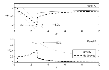
Figure 12: A comparison of ISSV solutions from different ODEs. Panel A presents $-v(x)$ versus $x$ profiles and panel B presents $\alpha(x)$ versus $x$ profiles. The light solid curves is a solution of ODEs (8) and (9) with self-gravity. The heavy dashed curves represent a solution of ODEs (24) and (25) without self-gravity. An equi-temperature shock with $\tau=1$ is introduced in both solutions at $x_{s}=2.7025$. The dotted curves in both panels represent the SCL. Other relevant parameters are contained in Table 6.

Table 6: Parameters for two ISSV solutions shown in Fig. 12

  Gravity $x_{0}$ $\alpha_{0}$ $x_{s}$ $V$ $A$ With $2.1$ $0.675$ $2.7025$ $0.2$ $1$ Without $0.37$ $0.191$ $2.7025$ $0.2$ $1$  

4.2 Formation of ISSV Edge

In our model, the central void region is simply treated as a vacuum with no materials inside. We need to describe astrophysical mechanisms responsible for creating such voids and for their local evolution. On the right side of the void edge $x_{0}^{+}$, the gas density $\alpha(x)>0$ for $x>x_{0}$, while $\alpha(x)=0$ for $x<x_{0}$. If no materials exist within the void edge, there would be no mechanism to confine the gas against the inward pressure force across the void edge. We offer two plausible astrophysical scenarios to generate and maintain such voids.

4.2.1 Energetics and Pressure Balance

If we allow a tenuous gas to exist within a ‘void’ region to counterbalance the pressure across the ‘void’ edge for a certain time $t$, transformation (5) gives the edge density $\rho_{0}$ as

$$\rho_{0}(t)=7.16\times 10^{8}\alpha_{0}\left(\frac{10^{3}\hbox{ yr}}{t}\right)^{2}m_{p}\ \ \hbox{cm}^{-3},$$ (26)

where $\alpha_{0}\equiv\alpha(x_{0})$ is the reduced mass density at ISSV edge and $m_{p}$ is the proton mass. For a gas temperature $T$, the isothermal sound speed $a$ is

$$a=2.87\times 10^{7}\bigg{(}\frac{T}{10^{7}\hbox{ K}}\bigg{)}^{1/2}\ \hbox{cm s}^{-1},$$ (27)

where the mean particle mass is that of hydrogen atom. Then the gas pressure $p_{0}$ just on the outer side of the ISSV edge is

$$p_{0}(t)=\rho_{0}a^{2}=0.99\alpha_{0}\left(\frac{10^{3}\hbox{ yr}}{t}\right)^{2}\frac{T}{10^{7}\hbox{ K}}\hbox{ dyne cm}^{-2},$$ (28)

where $\rho_{0}$ is the mass density at the ISSV edge. Here, we take the proton mass as the mean particle mass. Equation (28) gives a pressure scaling $p_{0}\propto t^{-2}T$ governed by self-similar hydrodynamics.

Within a ‘void’, we may consider that a stellar wind steadily blows gas outwards with a constant speed. Various astrophysical systems can release energies at different epochs. For an early evolution, massive stars steadily blow strong winds into the surrounding ISM (e.g. Mathews 1966; Dyson 1975; Falle 1975; Castor et al. 1975; Weaver et al. 1977). In the late stage of evolution, compact stars can also blow fast winds to drive the surrounding gas (e.g. Chevalier 1997a; Chevalier 1997b). As a model simplification, we assume that a tenuous gas moving outwards at constant speed $v_{w}$ with temperature $T_{w}$ (we refer to this as a central wind) may carve out a central ‘void’ and can provide a pressure against the pressure gradient across the ‘void’ boundary; suppose that this central wind begins to blow at time $t=0$. Then after a time $t$, the radius $r$ of the central wind front is at $r_{w}=v_{w}t$. By the mass conservation in a spherically symmetric flow, the mass density of the central wind front at time $t$ is then

$$\rho_{w,front}=\frac{\dot{M}}{4\pi v_{w}^{3}t^{2}}\ ,$$ (29)

where $\dot{M}$ is the mass loss rate of the central wind. For a contact discontinuity the ISSV edge between the inner stellar wind front and outer slower wind, the plasma pressure $p_{w,front}$ of this central fast wind is

$$p_{w,front}=\frac{k_{B}T_{w}}{m}\frac{\dot{M}}{4\pi v_{w}^{3}t^{2}}\ ,$$ (30)

which can be estimated by

$$\frac{4.16\times 10^{-6}\dot{M}}{10^{-6}M_{\odot}\hbox{ yr}^{-1}}\left(\frac{10\hbox{km s}^{-1}}{v_{w}}\right)^{3}\left(\frac{10^{3}\hbox{yr}}{t}\right)^{2}\frac{T_{w}}{10^{7}\hbox{K}}\hbox{dyne\ cm}^{-2},$$ (31)

where $M_{\odot}$ is the solar mass and the mean particle mass is that of hydrogen atom. We adopt the parameters based on estimates and numerical calculations (see Section 4.3). By expressions (30) and (31), the plasma pressure at the central wind front also scales as $p_{w,front}\propto t^{-2}T_{w}$. By a contact discontinuity between the central wind front and the ISSV edge with a pressure balance $p_{w,front}=p_{0}$, our self-similar ‘void’ plus the steady central wind can sustain an ISSV evolution as long as the central stellar wind can be maintained. Across such a contact discontinuity, the densities and temperatures can be different on both sides. Equations (31) and (28) also show that, while pressures balance across a contact discontinuity, the reduced density at ISSV edge $\alpha_{0}$ is determined by the mass loss rate $\dot{M}$ and central wind radial velocity $v_{w}$. Back into this steady central stellar wind of a tenuous plasma at a smaller radius, it is possible to develope a spherical reverse shock. This would imply an even faster inner wind inside the reverse shock (i.e. closer to the central star); between the reverse shock and the contact discontinuity is a reverse shock heated downstream part of the central stellar wind. Physically, the downstream portion of the central stellar wind enclosed within the contact discontinuity is expected to be denser, hotter and slower as compared with the upstream portion of the central stellar wind enclosed within the reverse shock.

The above scenario may be also adapted to supernova explosions. At the onset of supernova explosions, the flux of energetic neutrinos generated by the core collapse of a massive progenitor star could be the main mechanism to drive the explosion and outflows. This neutrino pressure, while different from the central wind plasma pressure discussed above, may be able to supply sufficient energy to drive rebound shocks in a dense medium that trigger supernova explosions (e.g. Chevalier 1997b; Janka et al. 2007; Lou & Wang 2006, 2007; Lou & Cao 2007; Arcones et al. 2008; Hu & Lou 2009). Under certain conditions, such neutrino pressure may even counterbalance the strong inward pressure force of an extremely dense gas and generate central ‘voids’. We will apply this scenario and give examples in Section 4.3.

4.2.2 Diffusion Effects

For astrophysical void systems with timescales of sufficient energy supply or pressure support being shorter than their ages, there would be not enough outward pressure at void edges to balance the inward pressure of the gas shell surrounding voids after a certain time. In such situations, the gas shell surrounding a central void will inevitably diffuse into the void region across the void edge or boundary. This diffusion effect will affect behaviours of void evolution especially in the environs of void edge and gradually smear the ‘void boundary’. However, because the gas shell has already gained a steady outward radial velocity before the central energy supply such as a stellar wind pressure support fails, the inertia of a dense gas shell will continue to maintain a shell expansion for some time during which the gas that diffuses into the void region accounts for a small fraction of the entire shell and outer envelope. As a result, it is expected that our ISSV solutions remain almost valid globally to describe void shell behaviours even after a fairly long time of insufficient central support.

We now estimate the gas diffusion effect quantitatively. We assume that a void boundary expands at $ax_{0}$ and the void is surrounded by a gas envelope whose density profile follows a $\rho(r)\propto r^{-2}$ fall-off (asymptotic solution 15). The gas shell expands at radial velocity $ax$ for $x>x_{0}$. The central energy supply mechanism has already maintained the void to a radius $r_{0}$ and then fails to resist the inward pressure across the void edge. We now estimate how many gas particles diffuse into void region in a time interval of $\Delta t=r_{0}/(ax_{0})$, during which the void is supposed to expand to a radius $2r_{0}$. We erect a local Cartesian coordinate system in an arbitrary volume element in gas shell with the $x-$axis pointing radially outwards. The Maxwellian velocity distribution of thermal particles gives the probability density of velocity $\overrightarrow{v}=(v_{x},v_{y},v_{z})$ as

$$p_{v}(\overrightarrow{v})\propto\exp{\left[-\frac{(v_{x}-ax_{0})^{2}+v_{y}^{2}+v_{z}^{2}}{2a^{2}}\right]}\ .$$ (32)

Define $l$ as the mean free path of particles in the gas shell near void edge. If a gas particle at radius $r$ can diffuse into radius $\tilde{r}$ without collisions, its velocity is limited by $(r+v_{x}\Delta t)^{2}+(v_{y}\Delta t)^{2}+(v_{z}\Delta t)^{2}<\tilde{r}^{2}$ and its position is limited by $r-\tilde{r}<l$. We simplify the velocity limitation by slightly increasing the interval as $(r+v_{x}\Delta t)^{2}<\tilde{r}^{2}$ and $v_{y}^{2}+v_{z}^{2}<(\tilde{r}/\Delta t)^{2}$. We first set $\tilde{r}=r_{0}$ and integrate the ratio of particles that diffuse into radius $r_{0}$ during $\Delta t$ to total gas shell particles within radius $r_{0}+l$ as

$$\!\!\!\!\frac{\int_{r_{0}}^{r_{0}+l}4\pi r^{2}\rho(r)dr\int_{\|r+v_{x}\Delta t\|<r_{0}\&v_{y}^{2}+v_{z}^{2}<(r_{0}/\Delta t)^{2}}p_{v}d^{3}v}{\int_{r_{0}}^{r_{0}+l}4\pi r^{2}\rho(r)dr\int p_{v}d^{3}v}\\ =\frac{1-\exp{\left[-r_{0}^{2}/(2a^{2}\Delta t^{2})\right]}}{(2\pi)^{1/2}l}\\ \qquad\qquad\times\int_{r_{0}}^{r_{0}+l}dr\int_{-\frac{r+r_{0}}{a\Delta t}-x_{0}}^{-\frac{r-r_{0}}{a\Delta t}-x_{0}}\exp{(-\tilde{v}^{2}/2)}d\tilde{v}\\ =\frac{1-\exp{(-x_{0}^{2}/2)}}{(2\pi)^{1/2}}\frac{r_{0}}{l}\\ \qquad\ \times\int_{1}^{1+l/r_{0}}d\tilde{x}\int_{-\tilde{x}-2x_{0}}^{-\tilde{x}}\exp{\left(-\tilde{v}^{2}/2\right)}d\tilde{v}\ ,$$ (33)

where both $\tilde{x}$ and $\tilde{v}$ are integral elements. We simply set $x_{0}=1$ and present computational results in Table 7. It is clear that even the inner energy supply fails to sustain inward pressure for a fairly long time, there are only very few particles that diffuse into the original void region, namely, a void remains quite empty.

In the context of PNe, the particle mean free path $l$ may be estimated for different species under various situations. For an example of PN to be discussed in Section 4.3.1, $l=1/(n\sigma)=3\times 10^{20}$ cm, where $n\approx 5000$ cm^-3 is the proton (electron) number density in the H II region and $\sigma=6.65\times 10^{-25}$ cm² is the electron cross section in Thomson scattering. One can also estimate cross section of coulomb interaction between two protons as $\sim 10^{-17}\hbox{ cm}^{2}$ and thus the mean free path for proton collisions is $\sim 10^{1}3$cm. A PN void radius is $\sim 5\times 10^{17}$ cm. If no inner pressure is acting further as a void expands to radius $\sim 10^{18}$ cm, gas particles that diffuse into $r\;\lower 4.0pt\hbox{${\buildrel\displaystyle<\over{\sim}}$}\;5\times 10^{17}$ cm only take up $\sim 6\times 10^{-5}$ of those in the gas shell. However, at the onset of a supernova explosion, the particle mean free path in the stellar interior is very small. If the density at a void edge is $\sim 1.2\times 10^{8}$ g cm^-3 (see Section 4.3.2), and the scattering cross section is estimated as the iron atom cross section $4.7\times 10^{-18}$ cm², the particle mean free path is only $l\sim 10^{-13}$ cm. Under this condition, particle that diffuse into a void region can account for $6.2\%$ of those in the total gas shell.

In short, while diffusion effect inevitably occurs when the inner pressure can no longer resist the inward gas pressure across a void edge, it usually only affects the gas behaviour near the void edge but does not alter the global dynamic evolution of gas shells and outer envelopes over a long time. However, we note that for a very long-term evolution, there will be more and more particles re-entering the void region when no sufficient pressure is supplied, and eventually the diffusion effect will result in significant changes of global dynamical behaviours of voids and shells. These processes may happen after supernova explosions. When neutrinos are no longer produced and rebound shocks are not strong enough to drive outflows, a central void generated in the explosion will gradually shrink in the long-term evolution of supernova remnants (SNRs).

Table 7: Ratio of molecules that diffuse into radius $r_{0}$ during $\Delta t$ to total gas shell molecules within radius $r_{0}+l$ under different ratio $l/r_{0}$. We take $x_{0}=1$.

  $l/r_{0}$ $+\infty$ $10$ $1$ $0.1$ $<<1$ ratio $3.6\%r_{0}/l$ $0.34\%$ $2.9\%$ $5.8\%$ $6.2\%$  

4.2.3 Applications of ISSV Model Solutions

In formulating the basic model, we ignore the gravity of the central void region. By exploring the physics around the void boundary, a tenuous gas is unavoidable inside a ‘void’ region for either an energy supply mechanism leading to an effective pressure or that diffused across the void boundary. As long as the gravity associated with such a tenuous gas inside the ‘void’ is sufficiently weak, our ISSV model should remain valid for describing the large-scale dynamic evolution of void shells, shocks, and outer envelopes.

In a planetary nebula or a supernova remnant, there is usually a solar mass compact star at the centre (e.g. Chevalier 1997a). For outgoing shells at a slow velocity of sound speed $\sim 10$ km s^-1, the Parker-Bondi radius of a central star of $10M_{\odot}$ is $\sim 10^{15}$ cm (i.e. $\sim 10^{-3}$ light year or $\sim 3\times 10^{-4}$ pc). The typical radius of a planetary nebula is about $10^{18}$ cm (see Section 4.3.1). Even the youngest known supernova remnant G1.9+0.3 in our Galaxy, estimated to be born $\sim 140$ yr ago, has a radius of $\sim 2$ pc (e.g. Reynolds 2008; Green et al. 2008). Thus the central star only affects its nearby materials and has little impact on gaseous remnant shells.

For a stellar wind bubble (e.g. Rosette Nebula), there usually are several, dozens or even thousands early-type stars blowing strong stellar winds in all directions. For example, the central ‘void’ region of Rosette Nebula contains the stellar cluster NGC 2244 of $\sim 2000$ stars (e.g. Wang et al. 2008). Conventional estimates show that the thick nebular shell has a much large mass of around $10$,$000-16$,$000$ solar masses (e.g. Menon 1962; Krymkin 1978). For a sound speed of $\sim 10$ km s^-1, the Parker-Bondi radius of a central object of $2000M_{\odot}$ is then $\sim 0.08$ pc, which is again very small compared to the $\sim 6$ pc central void in Rosette Nebula (e.g. Tsivilev et al. 2002). For a typical interstellar bubble consdiered in Weaver et al. (1977), the total mass inside the bubble, say, inside the dense shell, is no more than $50$ solar masses, which is significantly lower than that of the $2000$ solar mass dense shell.

We thus see that the dynamical evolution of flow systems on scales of planetary nebulae, supernova remnants and interstellar bubbles are only affected very slightly by central stellar mass objects (e.g. early-type stars, white dwarfs, neutron stars etc). Based on this consideration, we regard the grossly spherical region inside the outer dense shells in those astrophysical systems as a void in our model formulation, ignore the void gravity, emphasize the shell self-gravity and invoke the ISSV solutions to describe their dynamic evolution.

4.3 Astrophysical Applications

Our ISSV model is adaptable to astrophysical flow systems such as planetary nebulae, supernova explosions, supernova remnants, bubbles and hot bubbles on different scales.

4.3.1 Planetary Nebulae

In the late phase of stellar evolution, a star with a main-sequence mass $\;\lower 4.0pt\hbox{${\buildrel\displaystyle<\over{\sim}}$}\;8M_{\odot}$ makes a transition from an extended, cool state where it blows a slow dense wind to a compact, hot state where it blows a fast wind. The interaction between the central fast wind with the outer slow wind results in a dense shell crowding the central region which appears as a planetary nebula (e.g. Kwok, Purton & Fitzgerald 1978). The hot compact white dwarf star at the centre is a source of photoionizing radiation to ionize the dense shell (e.g. Chevalier 1997a). When the fast wind catches up the slow dense wind, a forward shock and a reverse shock will emerge on outer and inner sides of a contact discontinuity, respectively. As shown in Section 4.2.3, the gravity of central white dwarf and its fast steady wind is negligible for the outer dense wind. Practically, the region inside the contact discontinuity may be regarded approximately as a void. Meanwhile, the photoionizing flux is assumed to be capable of ionizing and heating the slow wind shell to a constant temperature (Chevalier 1997a), and the outer envelope, the cool AGB slow wind that is little affected by the central wind and radiation, can be also regarded approximately as isothermal. The constant temperatures of dense photoionized shell and outer envelope are usually different from each other which can be well characterized by the isothermal sound speed ratio $\tau$ (see Section 2.2). Thus the dynamic evolution of dense shell and outer AGB wind envelope separated by a forward shock is described by a type $\mathcal{Z}$ ISSV solution.

Within the contact discontinuity spherical surface, there is a steady downstream wind blowing outside the reverse shock front (e.g. Chevalier & Imamura 1983). Consistent with Section 4.2.1, we define $r_{w}$ as the radius where the downstream wind front reaches and $r_{r}$ as the radius of reverse shock. Within the radial range of $r_{r}<r<r_{w}$, i.e. in the downstream region of the reverse shock, we have a wind mass density

$$\rho_{w}(r,\ t)=\frac{\dot{M}}{4\pi v_{w}r^{2}}\ .$$ (34)

We define $a_{w,d(u)}$ and $T_{w,d(u)}$ as the sound speed and gas temperature on the downstream (upstream) side of the reverse shock and ratio $\tau_{w}\equiv a_{w,d}/a_{w,u}$ $=(T_{w,d}/T_{w,u})^{1/2}$ to characterize the reverse shock. For a reverse shock in the laboratory framework of reference given by shock conditions (16) and (17), we have in dimensional forms

$$\!\!\!\!\!\!\!u_{u,rs}-u_{rs}=\frac{1}{2}\left(v_{w}-u_{rs}+\frac{a_{w,d}^{2}}{v_{w}-u_{rs}}\right)\\ \!\!\!+\frac{1}{2}\left\{\left[\frac{(v_{w}-u_{rs})^{2}-a_{w,d}^{2}}{v_{w}-u_{rs}}\right]^{2}+4a_{w,d}^{2}\frac{\tau_{w}^{2}-1}{\tau_{w}^{2}}\right\}^{1/2}\!\!,\\ \!\!\!\!\!\!\!v_{w}-u_{rs}=\frac{1}{2}\left(u_{u,rs}-u_{rs}+\frac{a_{w,u}^{2}}{u_{u,rs}-u_{rs}}\right)\\ \!\!\!-\frac{1}{2}\left\{\left[\frac{(u_{u,rs}-u_{rs})^{2}-a_{w,u}^{2}}{u_{u,rs}-u_{rs}}\right]^{2}+4a_{w,u}^{2}(1-\tau_{w}^{2})\right\}^{1/2}\!\!,\\ \!\!\!\!\!\!\!\rho_{u,rs}=\frac{v_{w}-u_{rs}}{u_{u,rs}-u_{rs}}\rho_{d,rs}\ ,\\$$ (35)

where $u_{rs}$ is the outgoing speed of the reverse shock, $u_{u,rs}$ is the upstream wind velocity, $\rho_{u(d),rs}$ is the upstream (downstream) mass density, respectively. The first and second expressions in equation (35) are equivalent: the first expresses the upstream flow velocity in terms of the downstream parameters, while the second expresses the downstream flow velocity in terms of the upstream parameters. In solving the quadratic equation, we have chosen the physical solution, while the unphysical one is abandoned. Normally, in the downstream region $r_{r}<r<r_{w}$, the plasma is shock heated by the central faster wind with $\tau_{w}>1$. In the regime of an isothermal shock for effective plasma heating, we take $\tau_{w}=1$ (i.e. $a_{w,d}=a_{w,u}=a_{w}$) for a stationary reverse shock in the laboratory framework of reference, shock conditions (35) and (34) reduce to

$$\rho_{u,rs}=\frac{\dot{M}}{4\pi u_{u,rs}r_{r}^{2}}\ ,\qquad u_{u,rs}=\frac{a_{w}^{2}}{v_{w}}\ ,\qquad u_{rs}=0\ .$$ (36)

In this situation, the reverse shock remains stationary in space and this may shed light on the situation that an inner fast wind encounters an outer dense shell of slow speed. While a reverse shock always moves inwards relative to both upstream and downstream winds, either outgoing or incoming reverse shocks are physically allowed in the inner wind zone in the laboratory framework of reference. In the former situation, the reverse shock surface, contact discontinuity surface and forward shock surface all expand outwards steadily, with increasing travelling speeds, respectively. In the latter situation, the downstream wind zone, namely, the shocked hot fast wind zone expands both outwards and inwards, and eventually fills almost the entire spherical volume within the dense shell. The reverse shock here plays the key role to heat the gas confined within a planetary nebula to a high temperature, which is thus referred to as a hot bubble. In all situations, between the reverse shock and the contact discontinuity, the downstream wind has a constant speed, supplying a wind plasma pressure to counterbalance the inward pressure force across the contact discontinuity.

Here, type $\mathcal{Z}$ ISSV solutions are utilized to describe the self-similar dynamic evolution of gas shell outside the outgoing contact discontinuity. An outgoing forward shock propagates in the gas shell after the central fast wind hits the outer dense shell. According to properties of type $\mathcal{Z}$ ISSV solutions, there may be outflows (i.e. winds and breezes), static ISM or inflows (i.e. accretion flows and contractions) in the region outside the forward shock. The spatial region between the contact discontinuity and the forward shock is the downstream side of the forward shock.

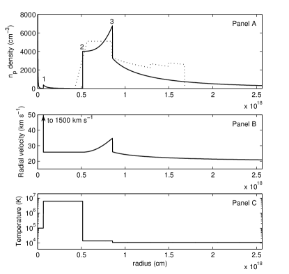
Figure 13: A type $\mathcal{Z}$ ISSV shock model with an inner fast wind to fit the planetary nebula NGC 7662. Panels A, B and C show our model results for proton number density $n_{\rm p}$, radial flow velocity and temperature of NGC 7662 in solid curve, respectively. Numerals $1$, $2$ and $3$ in Panel A mark reverse shock, contact discontinuity and forward shock surface, respectively. The dashed curve in Panel A is the estimate of proton number density by Guerrero et al. (2004). The inner fast wind blows at $1500$ km s^-1 inside the reverse shock, which is not shown in Panel B.

We now provide our quantitative model PN estimates for a comparison. Guerrero et al. (2004) probed the structure and kinematics of the triple-shell planetary nebula NGC 7662 based on long-slit echelle spectroscopic observations and Hubble Space Telescope archival narrowband images. They inferred that the nebula with a spatial size of $\sim 4\times 10^{18}$ cm consists of a central cavity surrounded by two concentric shells, i.e. the inner and outer shells, and gave a number density $n_{\rm p}$ distribution (the dotted curve in panel A of Figure 13). The temperatures of the inner and outer shells were estimated as $\sim 1.4\times 10^{4}$ K and $\sim 1.1\times 10^{4}$ K, respectively. No information about the inner fast wind is given in Guerrero et al. (2004). In our model consideration, the planetary nebula NGC 7662 may be described by our type $\mathcal{Z}$ ISSV model with a shocked inner fast wind. In our scenario for a PN, the central cavity in the model of Guerrero et al. (2004) should actually involve an inner fast wind region with a reverse shock. The inner and outer shells correspond to the downstream and upstream dense wind regions across a forward shock, respectively. Thus the inner boundary of the inner shell is the contact discontinuity in our model scenario. Physically, we suppose that the central star stops to blow a dense slow wind of $\sim 10$ km s^-1 about $\sim 1000$ years ago and the inner fast wind of $10^{5}$ K began to blow outwards from a white dwarf at $u_{u,rs}=1500$ km s^-1 about $\sim 600$ years ago. When the inner fast wind hits the dense slow wind $\sim 4$ years after its initiation, a reverse shock and a forward shock are generated on the two sides of the contact discontinuity. The reverse shock moves inwards at a speed $\sim 10$ km s^-1. The best density fit to the estimate of Guerrero et al. (2004) is shown in Figure 13. In our model, the inner fast wind has a mass loss rate from the compact star as $\sim 2\times 10^{-8}$M_⊙ yr^-1 (consistent with earlier estimates of Mellema 1994 and Perinotto et al. 2004) and the reverse shock is able to heat the downstream wind to a temperature of $\sim 6.4\times 10^{6}$ K. The downstream wind of the reverse shock has an outward speed of $\sim 25.9$ km s^-1, corresponding to a kinematic age (i.e. the time that a shocked fast wind at that velocity blows from the central point to its current position) of $\sim 630$ years. In Guerrero et al. (2004), the kinematic age is estimated to be $\sim 700$ years. In Guerrero et al. (2004), the inner shell density is $\sim 5\times 10^{3}$ $m_{\rm p}$ cm^-3 and our model shows a density variation from $\sim 4\times 10^{3}$ $m_{\rm p}$ cm^-3 to $\sim 7\times 10^{3}$ $m_{\rm p}$ cm^-3 with a comparable mean. The forward shock travels outwards at a speed $\sim 43.0$ km s^-1, consistent with an average outward velocity of the inner shell at $\sim 44$ km s^-1. The total mass of the inner shell is $\sim 8.5\times 10^{-3}$M_⊙, and the mass of the outer shell within a radius of $2.5\times 10^{18}$ cm is $\sim 0.036$M_⊙, which are all consistent with estimates of Guerrero et al. (2004). However, Guerrero et al. inferred that the outer shell has an outward velocity of around $50$ km s^-1 and a proton number density of $\sim 3000$ cm^-3. Our model estimates indicate that the outer shell has a proton number density from $3200$ cm^-3 at the immediate upstream side of the forward shock to $\sim 400$ cm^-3 at $2.5\times 10^{18}$ cm, and the outward velocity varies from $\sim 26$ km s^-1 at the upstream point of the forward shock to $\sim 20$ km s^-1 at $2.5\times 10^{18}$ cm. And thus the dense slow wind mass loss rate is $0.68\times 10^{-5}$M_⊙yr^-1, which is consistent with earlier numerical simulations (e.g. Mellema 1994; Perinotto et al. 2004), but is lower by one order of magnitude than $\sim 10^{-4}$M_⊙yr^-1 estimated by Guerrero et al. (2004). In summary, our ISSV model appears consistent with observations of the NGC 7662, and a combination of hydrodynamic model with optical and X-ray observations would be valuable to understand the structure and dynamic evolution of planetary nebulae.

4.3.2 Supernova Explosions and Supernova Remnants

At the onset of a type II supernova (or core-collapse supernova) for a massive progenitor, extremely energetic neutrinos are emitted by the neutronization process to form a ‘neutrino sphere’ that is deeply trapped by the nuclear-density core and may trigger a powerful rebound shock breaking through the heavy stellar envelope. At that moment, the central iron core density of a $\sim 15M_{\odot}$ progenitor star can reach as high as $\sim 7.3\times 10^{9}$ g cm^-3 and the core temperature could be higher than $\sim 7.1\times 10^{9}$ K. The density of the silicon layer is $\sim 4.8\times 10^{7}$ g cm^-3 with a temperature of $\sim 3.3\times 10^{9}$ K. The tremendous pressure produced by relativistic neutrinos may drive materials of such high density to explosion (e.g. Woosley & Janka 2005). During the first $\sim 10$ s of the core collapse, a power of about $\sim 10^{53}$ erg s^-1 is released as high-energy neutrinos within a radius of $\sim 10^{5}$ km (e.g. Woosley & Janka 2005). The neutrino-electron cross section was estimated to be $\sim 10^{-42}$(E/GeV)cm² with $E$ being the neutrino energy (e.g. Marciano & Parsa 2003). During the gravitational core collapse of a SN explosion, a typical value of E would be E$\sim$20MeV (e.g. Hirata et al. 1987; Arcones et al. 2008). Therefore, the neutrino-electron cross section is estimated to be $\sim 2\times 10^{-44}\hbox{ cm}^{2}$. If we adopt the neutrino luminosity $L=10^{53}\hbox{ erg s}^{-1}$, the ratio of neutrino pressure to one electron and the iron-core gravity on one silicon nucleus is $\sim 10^{-6}$. By these estimates, neutrino pressure is unable to split the silicon layer from the iron core. A pure vacuum void is unlikely to appear during the gravitational core collapse and the rebound process to initiate a SN.

During the subsequent dynamic evolution, diffusion effects would gradually smooth out any sharp edges and the inner rarefied region will be dispersed with diffused gaseous materials. Behaviour of this gas may be affected by the central neutron star. For example, a relativistic pulsar wind is able to power a synchrotron nebula referred to as the pulsar wind nebula, which is found within shells of supernova remnants (e.g. Gaensler et al. 1999). Pulsar winds relate to the magnetic field of pulsars and are not spherically symmetric. However, if the angle between magnetic and spin axes of a pulsar is sufficiently large and the pulsar is rapidly spinning, the averaged pressure caused by a pulsar wind may appear grossly spherical. This pulsar wind pressure may also counterbalance the inward pressure of outer gas and slow down the diffusion process. We offer a scenario that a supernova remnant makes a transition from a sharp-edged ‘void’ to a quasi-smooth one due to combined effects of diffusion and pulsar wind.

4.3.3 Interstellar Bubbles

Our ISSV model solutions may also describe large-scale nebula evolution around early-type stars or Wolf-Rayet stars. Here our overall scenario parallels to the one outlined in Section 4.3.1 for PNe but is different at the ambient medium surrounding the flow systems. For an interstellar bubble, a central stellar wind collides with the ISM (i.e. no longer a dense wind) and gives rise to a reverse shock that heats the downstream stellar wind zone, and a forward shock that propagates outwards in the ISM. Meanwhile, by inferences of radio and optical observations for such nebulae (e.g. Carina Nebula and Rosette Nebula), the central hot stars are capable of ionizing the entire swept-up shell and thus produce huge H II regions surrounding them (e.g. Menon 1962; Gouguenheim & Bottinelli 1964; Dickel 1974). The temperature of a H II region is usually regarded as weakly dependent on plasma density, thus an isothermal H II region should be a fairly good approximation (e.g. Wilson, Rohlfs & Hüttemeister 2008). As the ISM outside the forward shock is almost unaffected by the central wind zone, we may approximate the static ISM as isothermal and the dynamic evolution of gas surrounding interstellar bubbles can be well characterized by various ISSV solutions. Several prior models that describe ISM bubble shells in adiabatic expansions without gravity, might encounter problems. For example, the self-similar solution of Weaver et al. (1977) predicts a dense shell with a thickness of only $\sim 0.14$ times the radial distance from the central star to the shell boundary, which is indeed a very thin shell. However, observations have actually revealed many ISM bubbles with much thicker shells (e.g. Dorland, Montmerle & Doom 1986). The Rosette Nebula has a H II shell with a thickness of $\sim 20$ pc while the radius of central void is only $\sim 6$ pc (e.g. Tsivilev et al. 2002). The shell thickness thus accounts for $\sim 70\%$ of the radius of shell outer boundary, which is much larger than the computational result of Weaver et al. (1977). In our ISSV solutions, there are more diverse dynamic behaviours of gas shells and outer envelopes. For example in Figure 9, four ISSV solutions with static outer envelope indicate that the ratio of shell thickness to the radius of the forward shock covers a wide range. For these four solutions, this ratio is $0.65$, $0.98$, $0.91$ and $0.57$ respectively.

A type $\mathcal{Z}_{I}$ void shock solution with $x_{0}=0.58$, $\alpha_{0}=0.014$ and an isothermal shock at $x_{s}=2.2$ may characterize gross features of Rosette Nebula reasonably well. This ISSV solution indicates that when the constant shell temperature is $7000$ K (somewhat hotter than $6400$ K as inferred by Tsivilev et al. 2002) and the entire nebula system has evolved for $\sim 10^{6}$ years, the central void has a radius of $\sim 6.0$ pc; the forward shock outlines the outer shell radius as $\sim 22.8$ pc; the electron number density in the HII shell varies from $\sim 8.5$ cm^-3 to $\sim 12.9$ cm^-3; the contact discontinuity surface expands at a speed of $\sim 6.1$ km s^-1 and the forward shock propagates into the ISM at a speed of $\sim 16.4$ km s^-1; the surrounding ISM remains static at large radii. In the above model calculation, an abundance He$/$H ratio of $0.1/0.9$ is adopted. Various observations lend supports to our ISSV model results. For example, Tsivilev et al. (2002) estimated a bit higher shell electron number density as $15.3$ cm^-3 and an average shell expanding velocity of about $8.5$ km s^-1. Dorland et al. (1986) gave an average shell electron number density as $11.3$ cm^-3. Our calculation also gives a shell mass of $\sim 1.55\times 10^{4}M_{\odot}$, which falls within $10$,$000M_{\odot}$ and $16$,$000M_{\odot}$ as estimated by Menon (1962) and Krymkin (1978), respectively.

To study these inner voids embedded in various gas nebulae, diagnostics of X$-$ray emissions offers a feasible means to probe hot winds. The thermal bremsstrahlung and line cooling mechanisms can give rise to detectable X$-$ray radiation from optically thin hot gas (e.g. Sarazin 1986) and the high temperature interaction fronts of stellar winds with the ISM and inner fast wind with the void edge can produce X$-$ray photons (e.g. Chevalier 1997b). We will provide the observational properties of different types of voids and present diagnostics to distinguish the ISSV types and thus reveal possible mechanisms to generate and maintain such voids by observational inferences in a companion paper (Lou & Zhai 2009 in preparation).

5 Conclusions

We have explored self-similar hydrodynamics of an isothermal self-gravitating gas with spherical symmetry and shown various void solutions without or with shocks.

We first obtain type $\mathcal{X}$ ISSV solutions without shocks outside central voids in Section 3.3. Based on different behaviours of eigen-derivatives across the SCL, type $\mathcal{X}$ void solutions are further divided into two subtypes: types $\mathcal{X}_{\rm I}$ and $\mathcal{X}_{\rm II}$ ISSV solutions. All type $\mathcal{X}$ ISSV solutions are characterized by central voids surrounded by very dense shells. Both types $\mathcal{X}_{\rm I}$ and $\mathcal{X}_{\rm II}$ ISSV solutions allow envelope outflows but only type $\mathcal{X}_{\rm I}$ ISSV solutions can have outer envelopes in contraction or accretion flows.

We then consider self-similar outgoing shocks in gas envelopes surrounding central voids in Section 3.4. Type $\mathcal{Z}_{\rm I}$ void solutions are referred to as the equi-temperature shock solutions with a constant gas temperature across a shock front (this is an idealization; see Spitzer 1978). We also investigate various cases of shocks in type $\mathcal{Z}_{\rm II}$ void solutions (always a higher downstream temperature for the increase of specific entropy). In Section 3.4, we have developed the ‘phase net’ matching procedure to search for type $\mathcal{Z}$ ISSV solutions with static, expanding, contracting and accreting outer envelopes. ISSV solutions with quasi-smooth edges exist only when gas flows outwards outside the shock; all other types of voids are surrounded by fairly dense shells or envelopes.

We have systematically examined voids with sharp or quasi-smooth edges for various ISSV solutions. There must be some energetic processes such as supernova explosions or powerful stellar winds (including magnetized relativistic pulsar winds) that account for the appearance of sharp-edge voids. The denser the nebular shell is, the more difficult the void formation is. In other words, voids of quasi-smooth edges might be easier to form in the sense of a less stringent requirement for the initial energy input. In Section 4.1, we point out that the gas self-gravity can influence the void evolution significantly, especially for the property of regions near void edge as shown in Fig. 12. With the same boundary condition of outer medium, ISSV models with and without self-gravity can lead to different types of voids, e.g. quasi-smooth edge or sharp-edge voids. We suggest that these two types of voids may have different mechanisms to generate and sustain. Thus the inclusion of gas self-gravity is both physically realistic and essential. Besides, we show that all voids with quasi-smooth edges are type $\mathcal{Z}$ voids, that is, with shocks surrounding voids. This indicates that shock and expanding outer envelope may well imply a likely presence of a central void. In fact, observations on hot gas flows in clusters of galaxies might also be relevant in this regard. For example, McNamara et al. (2006) reported giant cavities and shock fronts in a distant ($z=0.22$) cluster of galaxies caused by an interaction between a synchrotron radio source and the hot gas around. Such giant X-ray cavities were reported to be left behind large-scale shocks in the galaxy cluster MS0735.6+7421.

Another point to note is that ISSV solutions we have constructed are physically plausible with special care taken for the expanding void boundary $x_{0}$. Void boundary $x_{0}$ involves density and velocity jumps not in the sense of a shock; local diffusion processes should happen to smooth out such jumps in a non-self-similar manner. Nonlinear ODEs (8) and (9) are valid in intervals $(0,\ x_{0}^{-})$ and $(x_{0}^{+},\ +\infty)$. We have indicated this property in Section 3.2 when introducing the concept of ISSV and discuss this issue in Section 4.2. There, several plausible mechanisms are noted such as powerful stellar winds and energetic neutrino driven supernova explosion. More specifically, we apply the ISSV solutions to grossly spherical planetary nebulae, supernova explosions or supernova remnants and interstellar bubbles.

Our model for planetary nebulae involve three characteristic interfaces: reverse shock, contact discontinuity surface, and forward shock. Steady inner stellar winds of different speeds blow on both sides of the inner reverse shock and a contact discontinuity surface confines the slower downstream wind zone outside the inner reverse shock. This reverse shock may be stationary or moving (either inwards or outwards) in the laboratory framework of reference. The contact discontinuity surface between the steady downstream wind zone (on the downstream side of the inner reverse shock) and the outer expanding gas shell moves outwards at a constant radial speed. Behaviours of outer shocked gas shell outside the contact discontinuity are described by type $\mathcal{Z}$ ISSV shock solutions with quasi-smooth edges. Stellar core collapses prior to supernova explosions lead to neutrino bursts during a short period of time, which might momentarily stand against the inward pressure force across the ‘void’ edge and give rise to a sharp-edge ‘void’ structure. In the long-term evolution after the escape of neutrinos, diffusion effect and outer forward shocks will dominate the behaviours of supernova remnants and the sharp edge will be smoothed out eventually. In other situations when central magnetized relativistic pulsar winds begin to resist diffusion effects, a quasi-smooth void with shocked shell (i.e. type $\mathcal{Z}$ ISSV) might also form.

Similar to PNe, interstellar bubbles may originate from strong stellar winds of early-type stars on larger scales. We invoke type $\mathcal{Z}$ ISSV solutions with quasi-smooth void edge to describe the structure and evolution of dense shell and outer ISM envelope. In our model, the hot shocked stellar wind zone, which is located between the reverse shock and the contact discontinuity surface, is filled with steady shocked wind plasma. In Weaver et al. (1977), the standard Spitzer conduction was included to study the shocked stellar wind and shell gas that diffuse into the shocked stellar wind region. However, the stellar magnetic field is predominantly transverse to the radial direction at large radii, which will suppress the thermal conduction through the hot interstellar bubble gas (e.g., Chevalier & Imamura 1983). As a weak magnetic field can drastically reduce this thermal conduction coefficient (e.g. Narayan & Medvedev 2001; Malyshkin 2001) and a weak magnetic field has little effects on behaviours of the gas shells and nebulae (e.g. Avedisova 1972; Falle 1975), we do not include thermal conduction effect in our model but present a dynamic evolution model for interstellar bubbles in terms of a self-similar nebular shell sustained by a central steady stellar wind. We would note that the existence of a random magnetic field may reduce the density ’wall’ around a void and make the formation of a void easier (Lou & Hu 2009). We do not include magnetic field in our model for simplicity.

Recent observations of ultraluminous X-ray sources (ULXs) show that ULXs may blow very strong winds or jets into the surrounding ISM and generate hot bubbles. For instance, ULX Bubble MH9-11 around Holmberg IX X-1 has experienced an average inflating wind/jet power of $\sim 3\times 10^{39}$ erg s^-1 over an age of $\sim 10^{6}$ years. The shock of the bubble travels outwards at $\sim 100$ km s^-1 at radius $\sim 100$ pc. The particle density around the shock is $\sim 0.3$ cm^-3 (e.g. Pakull & Grisé 2008). Approximately, this bubble corresponds to a type $\mathcal{Z}$ ISSV solution with $\alpha_{0}\approx 3.8\times 10^{-4}$, $x_{0}=0.4$ and $x_{s}=1$, and the temperature of gas shell is $\sim 10^{7}$ K. Our ISSV model predicts a contact discontinuity surface, or interaction surface of ULX wind with the ISM, at a radius $\sim 40$ pc.

Finally, to diagnose voids observationally, we would suggest among others to detect X$-$ray emissions from hot gas. In a companion paper), we shall adapt our ISSV solutions for hot optically thin X$-$ray gas clouds or nebulae, where we advance a useful concept of projected self-similar X$-$ray brightness. It is possible to detect ISSVs and identify diagnostic features of ISSV types which may in turn to reveal clues of ISSV generation mechanisms. We will also compare our ISSV model with observational data on more specific terms. Moreover, projected self-similar X$-$ray brightness is a general concept which can be useful when we explore other self-similar hydrodynamic or magnetohydrodynamic processes (e.g. Yu et al. 2006; Wang & Lou 2008).

Appendix A Jump of $\alpha$ from zero to
    nonzero value across the ZML

Let us assume that the reduced mass density $\alpha(x)$ can transit from zero to nonzero across the ZML and $x_{0}$ is the transition point. For this, we require $v(x_{0})=x_{0}$, $\alpha(x_{0})=0$ and when $x<x_{0}$, $\alpha(x)$ and $v(x)$ vanish. For an arbitrarily small real number $\varepsilon>0$, we also require $\alpha(x_{0}+\varepsilon)>0$ for a positive mass such that there exists a positive integer $n$ for which

$$\frac{d^{n}\alpha}{dx^{n}}\bigg{|}_{x_{0}}\neq 0\ .$$ (37)

We now cast equation (9) in the form of

$$\frac{d\alpha}{dx}=\alpha\frac{[\alpha-2(x-v)/x](x-v)}{(x-v)^{2}-1}\equiv\alpha{\cal F}(x)\ ,$$ (38)

where ${\cal F}(x)\equiv[\alpha-2(x-v)/x](x-v)/[(x-v)^{2}-1]$.

At $x=x_{0}$, the denominator of ${\cal F}(x)$ does not vanish because $v(x_{0})=x_{0}$. So ${\cal F}(x)$ is a finite continuous analytic function near $x_{0}$. An arbitrary order derivative of ${\cal F}(x)$ at $x_{0}$ should be finite as well.

The $k$th-order derivative of equation (A2) by the Leibnitz rule reads

$$\frac{d^{k+1}\alpha}{dx^{k+1}}=\sum_{i=0}^{k}C_{k}^{i}\frac{d^{i}\alpha}{dx^{i}}\frac{d^{k-i}{\cal F}(x)}{dx^{k-i}}\ ,$$ (39)

where $C_{k}^{i}$ stands for $k!/[i!(k-i)!]$ and $!$ is the standard factorial operation.

Because $\alpha(x_{0})=0$, equation (A3) yields $\alpha^{\prime}(x_{0})=0$, $\alpha^{\prime\prime}(x_{0})=0$ and so forth. That is, $\alpha(x_{0})=0$ and equation (9) determine that the arbitrary order derivative of $\alpha(x)$ at $x_{0}$ is zero, which is contrary to presumption (A1) based on the former assumption that $\alpha(x)$ can transit from zero to nonzero across $x_{0}$ of the ZML. Therefore $\alpha$ cannot transit from zero to nonzero across the ZML for an isothermal gas. For properties of void boundary in a polytropic gas, the interested reader is referred to Hu & Lou (2008) and Lou & Hu (2008).

Appendix B Proof of inequality $\alpha^{\prime\prime}(x_{0})<0$

Equation (9) can be written in the form of

$$\big{[}(x-v)^{2}-1\big{]}\alpha^{\prime}=\alpha\big{[}\alpha-2(1-v/x)\big{]}(x-v)\ ,$$ (40)

whose first-order derivative $d/dx$ is simply

$$\!\!\!\!\!\!\!\!\!2(x-v)(1-v^{\prime})\alpha^{\prime}+\big{[}(x-v)^{2}-1\big{]}\alpha^{\prime\prime}\\ \!\!\!\!\!\!\!\!\!=\{\alpha^{\prime}\big{[}\alpha-2(1-v/x)\big{]}+\alpha\big{[}\alpha^{\prime}+2v^{\prime}/x-2v/x^{2}\big{]}\}(x-v)\\ +\alpha\big{[}\alpha-2(1-v/x)\big{]}(1-v^{\prime})\ .$$ (41)

We have $v(x_{0})=x_{0}$ and thus both $v^{\prime}(x_{0})=0$ and $\alpha^{\prime}(x_{0})=0$ at $x_{0}$ by equation (22). Therefore at $x_{0}^{+}$, equation (B2) becomes

$$\alpha^{\prime\prime}(x_{0})=-\alpha(x_{0})^{2}<0\$$ (42)

for a positive density $\alpha(x_{0})>0$ as a physical requirement.

References

- (1) Abell G. O., 1966, ApJ, 144, 259
- (2) Alvarez M. A., Bromm V., Shapiro P. R., 2006, ApJ, 639, 621
- (3) Arcones A., Martínez-Pinedo G., O’Connor E., Schwenk A., Janka H.-Th., Horowitz C. J. Langanke K., 2008, Phys. Rev. C, 78, 015806
- (4) Avedisova V. S., 1972, Soviet Astr.-AJ, 15, 708
- (5) Band D. L., Liang E. P., 1988, ApJ, 334, 266
- (6) Bian F.-Y., Lou Y.-Q., 2005, MNRAS, 363, 1315
- (7) Castor J., McCray R., and Weaver R., 1975, ApJ, 200, L107
- (8) Chevalier R. A., 1982, ApJ, 259, 302
- (9) Chevalier R. A., Imamura J. N., 1983, ApJ, 270, 554
- (10) Chevalier R. A., 1997a, ApJ, 488, 263
- (11) Chevalier R. A., 1997b, Science, 276, 1374
- (12) Dorland H., Montmerle T., Doom C., 1986, A & A, 160, 1
- (13) Courant R., Friedrichs K. O., 1976, Supersonic Flow and Shock Waves. Springer-Verlag, New York
- (14) Dickel H. R., 1974, A&A, 31, 11
- (15) Dyson J. E., 1974, ApSS, 35, 299
- (16) Dyson J. E., Williams D. A., 1997, The Physics of the Interstellar Medium. IOP, Bristol and Philadelphia
- (17) Falle S. A. E. G., 1975, A&A, 43, 323
- (18) Fillmore J. A., Goldreich P., 1984, ApJ, 281, 9
- (19) Gaensler B. M., Gotthelf E. V., Vasisht G., 1999, ApJ, 526, L37
- (20) Goldreich P., Weber S. V., 1980, ApJ, 233, 991
- (21) Gouguenheim L., Bottinelli L., 1964, Ann. Astrophys, 27, 685
- (22) Green D. A., Reynolds S. P., Borkowski K. J., Hwang U., Harrus I., Petre R., 2008, MNRAS, 387, L54
- (23) Guerrero M. A., Jaxon E. G., Chu Y-H, 2004, ApJ, 128, 1705
- (24) Hirata K., et al., 1987, Phys. Rev. Lett, 58, 1490
- (25) Hu R.-Y., Lou Y.-Q., 2008, MNRAS, 390, 1619
- (26) Hu R.-Y., Lou Y.-Q., 2009, MNRAS, in press
- (27) Hunter C., 1977, ApJ, 218, 834
- (28) Hunter C., 1986, MNRAS, 223, 391
- (29) Janka H.-Th., Marek Andreas, Kitaura Francisco-Shu, 2007, Supernova 1987A: 20 Years After: Supernovae and Gamma-Ray Bursters. AIP Conference Proceedings, 937, 144
- (30) Kamper K. W., van den Bergh S., 1978, ApJ, 224, 851
- (31) Krymkin V. V., 1978, ApSS, 54, 187
- (32) Kwok S., Purton C. R., Fitzgerald P. M., 1978, ApJ, 219, L125
- (33) Kwok S., Volk K., 1985, ApJ, 299, 191
- (34) Landau L. D., Lifshitz E. M., 1987, Fluid Mechanics, 2nd ed., Pergamon Press, New York
- (35) Larson R. B., 1969a, MNRAS, 145, 271
- (36) Larson R. B., 1969b, MNRAS, 145, 405
- (37) Lou Y.-Q., Cao Y., 2008, MNRAS, 384, 611
- (38) Lou Y.-Q., Shen Y., 2004, MNRAS, 348, 717
- (39) Lou Y.-Q., Wang W.-G., 2006, MNRAS, 372, 885
- (40) Lou Y.-Q., Wang W.-G., 2007, MNRAS, 378, L54
- (41) Lou Y.-Q., Hu R.-Y., 2009, submitted
- (42) Malyshkin L., 2001, ApJ, 554, 561
- (43) Marciano W. J., Parsa Z., 2003, J. Phys. G: Nucl. Part. Phys. 29, 2629
- (44) Mathews W. G., 1966, ApJ, 144, 206
- (45) McNamara B. R., Nulsen P. E. J., Wise M. W., Rafferty D. A., Carilli C., Sarazin C. L., Blanton E. L., 2005, Nature, 433, 45
- (46) Mellema G., 1994, A&A, 290, 915
- (47) Menon T. K., 1962, ApJ, 135, 394
- (48) Meyer F., 1997, MNRAS, 285, L11
- (49) Narayan R., Medvedev M. V., 2001, ApJ, 562, L129
- (50) Pakull M. W., Grisé F., 2008, A Population Explosion: The Nature and Evolution of X-ray Binaries in Diverse Environments. AIP Conference Proceedings, Vol 1010, pp. 303-307 (arXiv:0803.4345v1 [astro-ph])
- (51) Penston M. V., 1969a, MNRAS, 144, 425
- (52) Penston M. V., 1969b, MNRAS, 145, 457
- (53) Perinotto M., Schönberner D., Steffen M., Calonaci C., 2004, A&A, 414, 993
- (54) Reynolds S. P., Borkowski K. J., Green D. A., Hwang U., Harrus I., Peter R., 2008, ApJ, 680, L41
- (55) Pikel’ner S. B., Shcheglov P. V., 1969, Soviet Astro.-AJ, 12, 757
- (56) Sarazin C. L., 1986, Review of Modern Physics, 58, 1
- (57) Shen Y., Lou Y.Q., 2004, ApJ, 611, L117
- (58) Shu F. H., 1977, ApJ, 214, 488
- (59) Shu F. H., Lizano S., Galli D., Cant J., Laughlin G., 2002, ApJ, 580, 969
- (60) Spitzer L., 1978, Physical Processes in the Interstellar Medium. Wiley, New York
- (61) Tsai J. C., Hsu J. J. L., 1995, ApJ, 448, 774
- (62) Tsivilev A. P., Poppi S., Cortiglioni S., Palumbo G. G. C., Orsini M., Maccaferri G., 2002, New Astronomy, 7, 449
- (63) Wang J., Townsley L. K., Feigelson E. D., Broos P., Getman K., Román-Zúñiga C. G., Lada E., 2008, ApJ, 675, 464
- (64) Wang W.-G., Lou Y.-Q., 2007, ApSS, 311, 363
- (65) Wang W.-G., Lou Y.-Q., 2008, ApSS, 315, 135
- (66) Weaver R., McCray R., Castor J., 1977, ApJ, 218, 377
- (67) Werner K., Rauch T., Kruk J. W., 2008, A&A, 492, L43
- (68) Whitworth A., Summers D., 1985, MNRAS, 214, 1
- (69) Wilson T. L., Rohlfs K., Hüttemeister S., 2008, Tools of Radio Astronomy, 5th ed., Springer Press
- (70) Woosley S., Janka T., 2005, Nature Physics, 1, 147
- (71) Yu C., Lou Y.-Q., 2005, MNRAS, 364, 1168
- (72) Yu C., Lou Y.-Q., Bian F.-Y., Wu Y., 2006, MNRAS, 370, 121