Superdeformed and hyperdeformed states in Z=122 isotopes

Abstract

We calculate the binding energy, root-mean-square radius and quadrupole deformation parameter for the recent, possibly discovered superheavey element Z=122, using the axially deformed relativistic mean field (RMF) and non-relativistic Skyrme Hartree-Fock (SHF) formalisms. The calculation is extended to include various isotopes of Z=122 element, strarting from A=282 to A=320. We predict highly deformed structures in the ground state for all the isotopes. A shape transition appears at about A=290 from a highly oblate to a large prolate shape, which may be considered as the superdeformed and hyperdeformed structures of Z=122 nucleus in the mean field approaches. The most stable isotope (largest binding energy per nucleon) is found to be ³⁰²122, instead of the experimentally observed ²⁹²122.

I Introduction

The stability of nuclei in superheavy mass region was predicted in mid sixties myers65 ; sobi66 ; mosel69 when shell correction was added to the liquid drop binding energy and the possible shell closure was pointed out at Z=114 and N=184. Myers and Swiatecki myers66 concluded that the half-lives of nuclei near the shell closures must be long enough to get observed. In other words, nuclei with zero shell effects would not be stable and decay immediately, as was predicted by macroscopic liquid drop models for Z$>$100 nuclides. Recentally, however, the spectroscopic studies of the nuclei beyond Z=100 have become possible herz04 , and the heaviest nucleus studied so far in this series of experiments herz06 is ²⁵⁴No (Z=102, N=152). Thus, the progress in experimental techniques has drawn our attention and opened up the field once again for further theoretical investigations in structure physics of nuclei in the superheavy mass region.

Even though, experimentally, the elements upto Z=118 have been synthesized to-date, with half-lives varying from few minutes to milliseconds hof00 ; oga07 , the above mentioned theoretically predicted center of island of stability could not be located precisely. Recently, more microscopic theoretical calculations have predicted various other regions of stability, namely, Z=120, N=172 or 184 rutz97 ; gupta97 ; patra1 and Z=124 or 126, N=184 cwiok96 ; kruppa00 . Apparently, there is a need to design the new experiments to solve the outstanding problem of locating the precise island of stability for superheavy elements. In an effort in this direction, using inductively coupled plasma-sector field mass spectroscopy, Marinov et al. marinov07 have observed some neutron-deficient Th isotopes in naturally occuring Thorium substances. Long-lived isomeric states, with estimated half-lives $T_{1/2}\geq$10⁸ y, have been identified in the neutron-deficient ^{211,213,217,218}Th isotopes, which are associated with the superdeformed (SD) or hyperdeformed (HD) states (minimma) in potential energy surfaces (PES). In a similar search for long-lived, trans-actinides in natural materials, more recently, these authors marinov09 obtained a possible evidence for the existence of a long-lived superheavy nucleus with mass number A=292 and atomic number Z=122 in natural Thorium. The half life is again estimated to be the same as above, i.e. $T_{1/2}\geq$10⁸ y and abundance (1-10)$\times$10^-12 relative to ²³²Th. This possibility of an extremely heavey Z nucleus motivated us to see the structures of such nuclei in an isotopic mass chain. Therefore, based on the relativistic mean-field (RMF) and non-relativistic Skyrme Hartree-Fock (SHF) methods, we calculated the bulk proporties of Z=122 nucleus in an isotopic chain of mass A=282-320. This choice of mass range covers both the predicted neutron magic numbers N=172 and 184.

The paper is organised as follows: Section II gives a brief description of the relativistic and non-relativistic mean-field formalisms. The effects of pairing for open shell nuclei, included in our calculations, are also discussed in this section. The results of our calculations are presented in Section III, and a summary of the results obtained, together with concluding remarks, are given in the last Section IV.

II Theoretical framework

II.1 The Skyrme Hartree-Fock (SHF) method

The general form of the Skyrme effective interaction, used in the mean-field models, can be expressed as an energy density functional $\cal H$, given as a function of some empirical parameters cha97 ; stone07 , as

$${\mathcal{H}}={\mathcal{K}}+{\mathcal{H}}_{0}+{\mathcal{H}}_{3}+{\mathcal{H}}_{eff}+\cdots$$ (1)

where ${\cal K}$ is the kinetic energy term, ${\cal H}_{0}$ the zero range, ${\cal H}_{3}$ the density dependent and ${\cal H}_{eff}$ the effective-mass dependent terms, which are relevant for calculating the properties of nuclear matter. These are functions of 9 parameters $t_{i}$, $x_{i}$ ($i=0,1,2,3$) and $\eta$, given as

$${\mathcal{H}}_{0} = \frac{1}{4}t_{0}\left[(2+x_{0})\rho^{2}-(2x_{0}+1)(\rho_{p}^{2}+\rho_{n}^{2})\right],$$ (2)

$${\mathcal{H}}_{3} = \frac{1}{24}t_{3}\rho^{\eta}\left[(2+x_{3})\rho^{2}-(2x_{3}+1)(\rho_{p}^{2}+\rho_{n}^{2})\right],$$ (3)

$${\mathcal{H}}_{eff} = \frac{1}{8}\left[t_{1}(2+x_{1})+t_{2}(2+x_{2})\right]\tau\rho$$

$$+\frac{1}{8}\left[t_{2}(2x_{2}+1)-t_{1}(2x_{1}+1)\right](\tau_{p}\rho_{p}+\tau_{n}\rho_{n}).$$

The kinetic energy ${\cal K}=\frac{\hbar^{2}}{2m}\tau$, a form used in the Fermi gas model for non-interacting fermions. Here, $m$ is the nucleon mass. The other terms, representing the surface contributions of a finite nucleus with $b_{4}$ and $b^{\prime}_{4}$ as additional parameters, are

$${\mathcal{H}}_{S\rho} = \frac{1}{16}\left[3t_{1}(1+\frac{1}{2}x_{1})-t_{2}(1+\frac{1}{2}x_{2})\right](\vec{\nabla}\rho)^{2}$$ (5)

$$-\frac{1}{16}\left[3t_{1}(x_{1}+\frac{1}{2})+t_{2}(x_{2}+\frac{1}{2})\right]$$

$$\times\left[(\vec{\nabla}\rho_{n})^{2}+(\vec{\nabla}\rho_{p})^{2}\right],\text{ and}$$

$${\mathcal{H}}_{S\vec{J}} = -\frac{1}{2}\left[{b_{4}}\rho\vec{\nabla}\cdot\vec{J}+{b^{\prime}_{4}}(\rho_{n}\vec{\nabla}\cdot\vec{J_{n}}+\rho_{p}\vec{\nabla}\cdot\vec{J_{p}})\right].$$ (6)

Here, the total nucleon number density $\rho=\rho_{n}+\rho_{p}$, the kinetic energy density $\tau=\tau_{n}+\tau_{p}$, and the spin-orbit density $\vec{J}=\vec{J}_{n}+\vec{J}_{p}$. The subscripts $n$ and $p$ refer to neutron and proton, respectively. The $\vec{J}_{q}=0$, $q=n$ or $p$, for spin-saturated nuclei, i.e., for nuclei with major oscillator shells completely filled. The total binding energy (BE) of a nucleus is the integral of the energy density functional $\cal H$.

At least eighty-seven parametrizations of the Skyrme interaction are published since 1972 (see, e.g., stone03 ). In most of the Skyrme parameter sets, the coefficients of the spin-orbit potential $b_{4}=b^{\prime}_{4}=W_{0}$ rei92 , but we have used here the Skyrme SkI4 set with $b_{4}\neq b^{\prime}_{4}$ rei95 . This parameter set is designed for considerations of proper spin-orbit interaction in finite nuclei, related to the isotope shifts in Pb region.

II.2 The relativistic mean-field (RMF) method

The relativistic Lagrangian density for a nucleon-meson many-body system sero86 ; ring90 ,

$${\cal L} = \overline{\psi_{i}}\{i\gamma^{\mu}\partial_{\mu}-M\}\psi_{i}+{\frac{1}{2}}\partial^{\mu}\sigma\partial_{\mu}\sigma-{\frac{1}{2}}m_{\sigma}^{2}\sigma^{2}$$ (7)

$$-{\frac{1}{3}}g_{2}\sigma^{3}-{\frac{1}{4}}g_{3}\sigma^{4}-g_{s}\overline{\psi_{i}}\psi_{i}\sigma-{\frac{1}{4}}\Omega^{\mu\nu}\Omega_{\mu\nu}$$

$$+{\frac{1}{2}}m_{w}^{2}V^{\mu}V_{\mu}+{\frac{1}{4}}c_{3}(V_{\mu}V^{\mu})^{2}-g_{w}\overline{\psi}_{i}\gamma^{\mu}\psi_{i}V_{\mu}$$

$$-{\frac{1}{4}}\vec{B}^{\mu\nu}.\vec{B}_{\mu\nu}+{\frac{1}{2}}m_{\rho}^{2}{\vec{R}^{\mu}}.{\vec{R}_{\mu}}-g_{\rho}\overline{\psi}_{i}\gamma^{\mu}\vec{\tau}\psi_{i}.\vec{R^{\mu}}$$

$$-{\frac{1}{4}}F^{\mu\nu}F_{\mu\nu}-e\overline{\psi}_{i}\gamma^{\mu}\frac{\left(1-\tau_{3i}\right)}{2}\psi_{i}A_{\mu}.$$

All the quantities have their usual well known meanings. From the above Lagrangian we obtain the field equations for the nucleons and mesons. These equations are solved by expanding the upper and lower components of the Dirac spinors and the boson fields in an axially deformed harmonic oscillator basis with an initial deformation $\beta_{0}$. The set of coupled equations is solved numerically by a self-consistent iteration method. The centre-of-mass motion energy correction is estimated by the usual harmonic oscillator formula $E_{c.m.}=\frac{3}{4}(41A^{-1/3})$. The quadrupole deformation parameter $\beta_{2}$ is evaluated from the resulting proton and neutron quadrupole moments, as $Q=Q_{n}+Q_{p}=\sqrt{\frac{16\pi}{5}}(\frac{3}{4\pi}AR^{2}\beta_{2})$. The root mean square (rms) matter radius is defined as $\langle r_{m}^{2}\rangle={1\over{A}}\int\rho(r_{\perp},z)r^{2}d\tau$, where $A$ is the mass number, and $\rho(r_{\perp},z)$ is the deformed density. The total binding energy and other observables are also obtained by using the standard relations, given in ring90 . We use the well known NL3 parameter set lala97 . This set not only reproduces the properties of stable nuclei but also well predicts for those far from the $\beta$-stability valley. As outputs, we obtain different potentials, densities, single-particle energy levels, radii, deformations and the binding energies. For a given nucleus, the maximum binding energy corresponds to the ground state and other solutions are obtained as various excited intrinsic states.

II.3 Pairing Effect

Pairing is a crucial quantity for open shell nuclei in determining the nuclear properties. The constant gap, BCS-pairing approach is reasonably valid for nuclei in the valley of $\beta$-stability line. However, this approach breaks down when the coupling of the continum becomes important. In the present study, we deal with nuclei on the valley of stability line since the superheavy elements, though very exotic in nature, lie on the $\beta$-stability line. These nuclei are unstable, because of the repulsive Coulomb force, but the attractive nuclear shell effects come to their resque, making the superheavy element possible to be synthesized, particularly when a combination of magic proton and neutron number happens to occur (largest shell correction). In order to take care of the pairing effects in these nuclei, we use the constant gap for proton and neutron, as given in madland81 : $\triangle_{p}=RB_{s}e^{sI-tI^{2}}/Z^{1/3}$ and $\triangle_{n}=RB_{s}e^{-sI-tI^{2}}/A^{1/3}$, with $R$=5.72, $s$=0.118, $t$= 8.12, $B_{s}$=1, and $I=(N-Z)/(N+Z)$. This type of prescription for pairing effects, both in RMF and SHF, has already been used by us and many others authors patra01 . For this pairing approach, it is shown patra01 ; lala99 that the results for binding energies and quadrople deformations are almost identical with the predictions of relativistic Hartree-Bogoliubov (RHB) approach.

III Results and Discussion

Ground state properties using the SHF and RMF models:
There exists a number of parameter sets for solving the standard SHF Hamiltonians and RMF Lagrangians. In many of our previous works and of other authors patra1 ; ring90 ; lala97 ; patra2 ; patra3 ; patra4 the ground state properties, like the binding energies (BE), quadrupole deformation parameters $\beta_{2}$, charge radii ($r_{c}$), and other bulk properties, are evaluated by using the various non-relativistic and relativistic parameter sets. It is found that, more or less, most of the recent parameter sets reproduce well the ground state properties, not only of stable normal nuclei but also of exotic nuclei which are far away from the valley of $\beta$-stability. This means that if one uses a reasonably acceptable parameter set, the predictions of the model will remain nearly force independent.

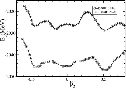
Figure 1: The potential energy surfaces for ²⁹²122 nucleus as a function of quadrupole deformation parameter. The circles with solid-line is for SHF using SkI4 parameter set, and the squares with dash-line is for RMF calculations using NL3 parameter set.

III.1 Potential energy surface

In this subsection, we first calculate the potential energy surfaces (PES) by using both the RMF and SHF theories in a constrained calculation patra4 ; flocard73 ; koepf88 ; reinhard89 ; hirata88 , i.e., instead of minimizing the $H_{0}$, we have minimized $H^{\prime}=H_{0}-\lambda Q_{2}$, with $\lambda$ as a Lagrange multiplier and $Q_{2}$, the quadrupole moment. Thus, we calculate the binding energy corresponding to the solution at a given quadrupole deformation. Here, $H_{0}$ is the Dirac mean field Hamiltonian (the notations are standard and its form can be seen in Refs. ring90 ; koepf88 ; hirata88 ) for RMF model and it is a Schrödinger mean field Hamiltonian for SHF model. In other words, we get the constrained binding energy from $E_{c}=\sum_{ij}\frac{<\psi_{i}|H_{0}-\lambda Q_{2}|\psi_{j}>}{<\psi_{i}|\psi_{j}>}$ and the “free energy” from $BE=\sum_{ij}\frac{<\psi_{i}|H_{0}|\psi_{j}>}{<\psi_{i}|\psi_{j}>}$. In our calculations, the free energy solution does not depend on the initial guess value of the basis deformation $\beta_{0}$ as long as it is nearer to the minimum in PES. However it converges to some other local minimum when $\beta_{0}$ is drastically different, and in this way we evaluate a different isomeric state for a given nucleus.

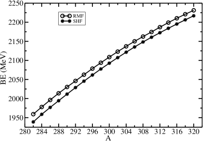
Figure 2: The total binding energy for ^282-320122 nuclei in SHF(SkI4) and RMF(NL3) calculations.

The PES, i.e., the potential energy as a function of quadrupole deformation parameter $\beta_{2}$, for the superheavy nucleus ²⁹²122, is shown in Fig. 1. Both the RMF and SHF results are given for comparisons. The calculated PES is shown for a wide range of oblate to prolate deformations. We notice from this figure that in RMF, minima appear at around $\beta_{2}$= -0.436, -0.032 and 0.523. The energy differences between the ground and the isomeric states are found to be 0.48 and 1.84 MeV for the nearest consucative minimas. For SHF, the minima appear at around $\beta_{2}$= -0.459,-0.159 and 0.511. The intrinsic excited state energy differences are 1.30 and 0.48 MeV. From the figure it is clear that the mimima and the maxima in both the RMF and SHF are qualitatively similar. The absolute value differ by a constant factor from one another, i.e., if we scale the lower curve by, say, a scaling factor c= 1.0075 then both the curves will coincide with each other. This difference in energy is also reflected in the binding energy calculations of this nucleus in an isotopic chain, which will be discussed in the following subsection.

Table 1: The SHF(SkI4) and the RMF(NL3) results for binding energy BE, two-neutron separation energy $S_{2n}$ and the quadrupole deformation parameter $\beta_{2}$, compared with the Finite Range Droplet Model (FRDM) data moll97 . The energy is in MeV.

	SHF(SkI4 parameter set)			RMF(NL3 parameter set)			FRDM results
Nucleus	BE	$S_{2n}$	$\beta_{2}$	BE	$S_{2n}$	$\beta_{2}$	BE	$S_{2n}$	$\beta_{2}$
294	2062.49	16.29	0.534	2045.52	16.71	0.530	2053.16		-0.155
296	2078.46	15.94	0.529	2061.74	16.21	0.527	2068.99	15.84	-0.130
298	2093.81	15.34	0.526	2077.44	15.70	0.536	2084.26	15.26	-0.096
300	2108.67	14.81	0.526	2092.62	15.18	0.548	2099.64	15.38	0.009
302	2123.01	14.34	0.529	2107.30	14.68	0.562	2113.98	14.34	0.418
304	2136.83	13.82	0.545	2121.47	14.17	0.603	2126.87	12.89	0.000
306	2150.03	13.20	0.556	2135.23	13.76	0.608	2139.43	12.56	0.000
308	2162.49	12.45	0.560	2148.30	13.08	0.618	2150.84	11.41	0.001
310	2174.49	12.00	0.571	2160.66	12.35	0.641	2162.05	11.22	0.003
312	2187.10	12.62	0.584	2172.58	11.92	0.742	2173.42	11.36	0.005
314	2199.12	12.02	0.594	2184.17	11.59	0.739	2184.67	11.25	0.006
316	2210.49	11.37	0.595	2195.39	11.22	0.736	2195.74	11.07	0.007
318	2221.02	10.65	0.588	2206.30	10.91	0.722	2214.11	18.37	0.541
320	2231.23	10.21	0.575	2216.96	10.67	0.728	2224.88	10.76	0.543

III.2 Binding energy and Two-neutron separation energy

Fig. 2 shows the calculated binding energy, obtained in both the SHF and RMF formalisms. We notice that, similar to the PES, the binding energy obtained in the RMF model also over-estimates the SHF result by a constant factor. In other words, here also the multiplication by a constant factor ’c’ will make the two curves overlap with one another. This means that a slight modification of the parameter set of one formalism can predict the binding energy similar to that of the other.

Table I shows a comparison of the calculated binding energies with the Finite Range Droplet Model (FRDM) predictions of Ref. moll97 , wherever possible. The two-neutron separation energy $S_{2n}$(N,Z)=BE(N,Z)-BE(N-2,Z) is also listed in Table I. From the table, we find that the microscopic binding energies and the $S_{2n}$ values agree well with the macro-microscopic FRDM calculations.

The comparison of $S_{2n}$ for the SHF and RMF with the FRDM result are further shown in Fig. 3, which shows clearly that the two $S_{2n}$ values coincide remarkably well, except at mass A=318 which seems spurious due to some error somewhere in the case of FRDM. Apparently, the $S_{2n}$ decrease gradually with increase of neutron number, except for the noticeable kinks at A=294 (N=172) and 312 (N=190) in RMF, and at A=304 (N=182) and 308 (N=186) in FRDM. Interestingly, these neutron numbers are close to either N=172 or 184 magic numbers. However, the SHF results are smooth.

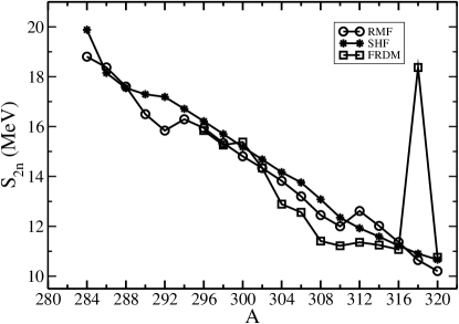
Figure 3: The two-neutron separation energy ${S_{2}n}$ for ^282-320122 nuclei, obtained from SHF(SkI4) and RMF(NL3) formalisms, and compared with the FRDM results moll97 , whereever available.

The binding energy per particle for the isotopic chain is also plotted in Fig. 4. We notice that here again the SHF and RMF curves could be overlapped with one another through a constant scaling factor, and the FRDM calculation lie in between these two calculations. This means, qualitatively, all the three curves show a similar behavior. However, unlike the BE/A curve for SHF or RMF, the FRDM results do not show the regular behaviour. In general, the BE/A start increasing with the increase of mass number A, reaching a peak value at A=302 for all the three formalisms. This means that ³⁰²122 is the most stable element from th binding energy point of view. Interestingly, ³⁰²122 is situated towards the neutron deficient side of the isotopic series of Z=122, and could be taken as a suggestion to synthesize this superheavy nucleus experimently.

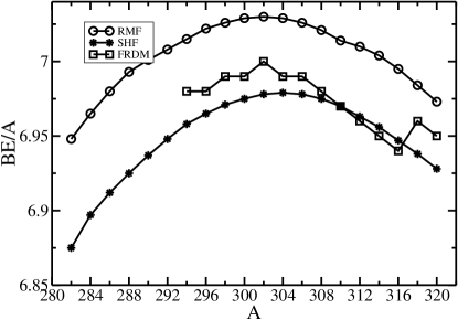
Figure 4: The binding energy per particle BE/A for the superheavy isotopes ^282-320122, obtained in SHF(SkI4) and RMF(NL3) formalisms, compared with the FRDM results moll97 , whereever available.

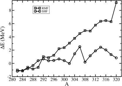
Figure 5: The energy difference between the ground state and the first excited state both in nonrelativistic SHF(SkI4) and relativistic RMF(NL3) formalisms.

Also, we have calculated the ”free solutions” for the whole isotopic chain, both in prolate and oblate deformed configurations. In many cases, we find low lying excited states. As a measure of the energy difference between the ground band and the first excited state, we have plotted in Fig. 5 the binding energy difference $\triangle E$ between the two solutions, noting that the maximum binding energy solution refers to the ground state and all other solutions to the intrinsic excited state(s). From Fig. 5, we notice that in RMF calculations, the energy difference $\triangle E$ is small for neutron-deficient isotopes, but it increases with the increase of mass number A in the isotopic series. On the other hand, in SHF formalism, $\triangle E$ value remains small throughout the isotopic chain. This later result means to suggest that the ground state can be changed to the excited state and vice-versa by a small change in the input, like the pairing strength, etc., in the calculations. In any case, such a phenomenon is known to exist in many other regions of the periodic table.

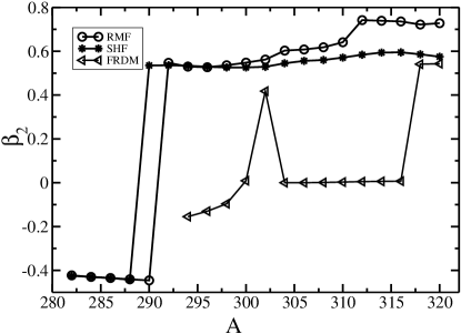
Figure 6: Comparision of quadrupole deformation parameter obtained from nonrelativistic SHF(SkI4) and relativistic mean field formalism RMF(NL3), compared with the FRDM results moll97 , whereever available.

III.3 Quadrupole deformation parameter

The quadrupole deformation parameter $\beta_{2}$, for both the ground and first excited states, are also determined within the two formalisms. In some of the earlier RMF and SHF calculations, it was shown that the quadrupole moment obtained from these theories reproduce the experimental data pretty well patra1 ; cha97 ; rei95 ; sero86 ; ring90 ; lala97 ; patra2 ; cha98 ; brown98 . We have seen in Fig. 1 that both the ground-state and intrinsic excited quadrupole deformation parameters for SHF and RMF results agree well with each other (the same is true for “free solutions”, not shown here). However, the ground-state (g.s.) quadrupole deformation parameter $\beta_{2}$ plotted in Fig. 6 for SHF and RMF, and compared with FRDM results moll97 , show that the FRDM results differ strongly. Both in the SHF and RMF results, we find highly deformed oblates solutions in the g.s. confuguration for isotopes near the low mass region. Then, with increase of mass number there is a shape change from highly oblate to highly prolate in both SHF and RMF models. Interestingly, most of the isotopes are superdeformed in their g.s. confugurations, and due to the shape co-existance proporties of these isotopes, some time it is possible that the g.s. could be the hyperdeformed solution.

Table 2: The $Q_{\alpha}$ and $T_{\alpha}$ calculated on the SHF(SkI4) and the RMF(NL3) models, and compared with the Finite Range Droplet Model (FRDM) results moll97 , whereever available. The energy is in MeV.

		SHF(SkI4 parameter set)			RMF(NL3 parameter set)			FRDM results
Nucleus	Z	BE	$Q_{\alpha}$	$T_{\alpha}$	BE	$Q_{\alpha}$	$T_{\alpha}$	BE	$Q_{\alpha}$	$T_{\alpha}$
292	122	2028.81	14.31	$10^{-7.23}$	2046.19	13.83	$10^{-6.35}$
288	120	2014.82	13.13	$10^{-5.49}$	2031.75	12.35	$10^{-3.85}$	2023.06	13.98	$10^{-6.07}$
284	118	1999.65	14.86	$10^{-9.11}$	2015.80	12.87	$10^{-5.48}$	2008.69	12.70	$10^{-4.08}$
280	116	1986.21	13.89	$10^{-7.93}$	2000.37	12.92	$10^{-6.10}$	1993.49	12.42	$10^{-5.10}$
276	114	1971.80	12.30	$10^{-5.37}$	1984.99	11.82	$10^{-4.33}$	1977.62	12.33	$10^{-5.44}$
272	112	1955.80	12.33	$10^{-5.97}$	1968.51	11.45	$10^{-4.07}$	1961.66	11.61	$10^{-4.45}$
268	110	1939.83	11.86	$10^{-5.54}$	1951.66	10.92	$10^{-3.41}$	1944.97	10.94	$10^{-3.47}$
264	108	1923.39	10.25	$10^{-2.34}$	1934.28	10.19	$10^{-2.19}$	1927.62	10.57	$10^{-3.18}$
260	106	1905.34	9.59	$10^{-1.10}$	1916.17	9.98	$10^{-2.27}$	1909.90	9.93	$10^{-2.15}$
256	104	1886.63	9.71	$10^{-2.20}$	1897.85	7.53	$10^{4.95}$	1891.53	8.75	$10^{0.59}$
252	102	1868.04	8.71	$10^{0.02}$	1877.08	8.02	$10^{2.32}$	1871.98	8.35	$10^{1.19}$
248	100	1848.45	7.34	$10^{4.08}$	1856.80	7.18	$10^{4.72}$	1852.03	7.64	$10^{2.91}$
244	98	1827.49	7.37	$10^{3.14}$	1835.68	6.85	$10^{5.26}$	1831.38	6.90	$10^{5.01}$
240	96	1806.56	6.63	$10^{3.34}$	1814.23	5.91	$10^{8.82}$	1809.98	6.52	$10^{5.81}$
236	94	1784.89	6.10	$10^{5.90}$	1791.84	5.64	$10^{9.26}$	1788.21	5.77	$10^{8.54}$
232	92	1762.69	6.09	$10^{5.98}$	1768.19	5.54	$10^{8.82}$	1754.15	5.14	$10^{11.18}$

III.4 Nuclear radii

The root mean square (rms) radius for proton ($r_{p}$), neutron ($r_{n}$) and matter distribution ($r_{m}$), both in SHF and RMF formalisms, is shown in Fig. 7. The upper pannel is for the SHF and the lower one for the RMF calculations. As expected, the neutron and matter distribution radius increases with increase of the neutron number. Although, the proton number Z=122 is constant in the isotopic series, the value of $r_{p}$ also increase as shown in the figure. This trend is similar in both the formalisms. A minute inspection of the figure shows that, in RMF calculation, the radii show a jump at A=312 (N=190) after the monotonous increase of radii till A=310. Note that a similar trend was observed in RMF calculations for $S_{2n}$ (see, Fig. 3).

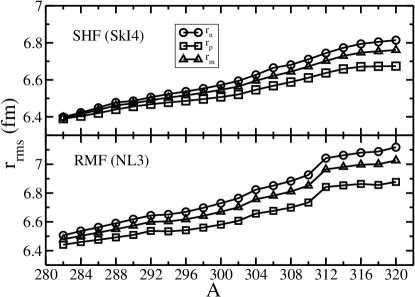
Figure 7: The rms radii of proton ($r_{p}$), neutron ($r_{n}$) and matter ($r_{m}$) distribution for ^282-320122 nuclei using nonrelativistic SHF(SkI4) and relativistic mean field formalism RMF(NL3).

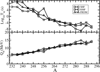
Figure 8: The half-life time $T_{\alpha}$ and the $Q_{\alpha}$ energy for ²⁹²122 nucleus, using the non-relativistic SHF(SkI4), the relativistic mean field formalism RMF(NL3), and the FRDM data moll97 .

III.5 The $Q_{\alpha}$ energy and the decay half-life $T_{\alpha}$

We choose the nucleus ²⁹²122 (Z=122, N=170) for illustrating our calculations of the $\alpha$-decay chain and the half-life time $T_{\alpha}$. The $Q_{\alpha}$ energy is obtained from the relation patra23 :

$$Q_{\alpha}(N,Z)=BE(N,Z)-BE(N-2,Z-2)-BE(2,2).$$

Here, $BE(N,Z$)is the binding energy of the parent nucleus with neutron number $N$ and proton number $Z$, $BE(2,2)$ is the binding energy of the $\alpha$-particle (${}^{4}He$) and $BE(N-2,Z-2)$ is the binding energy of the daughter nucleus after the emission of an $\alpha$-particle.

The binding energy of the parent and daughter nuclei are obtained by using both the RMF and SHF formalisms. Our predicted results are compared in Table II with the finite range droplet model (FRDM) calculation of Ref. moll97 . The $Q_{\alpha}$ values are then calculated, also shown in Table II and in lower panel of Fig. 8. Then, the half-life $Log_{10}T_{\alpha}(s)$ are estimated by using the phenomenological formulla of Viola and Seaborg viol01 :

$$Log_{10}T_{\alpha}(s)=\frac{aZ-b}{\sqrt{Q_{\alpha}}}-(cZ+d)$$

where Z is the atomic number of parent nucleus, $a$=1.66175, $b$=8.5166, $c$=0.20228 and $d$=33.9069. The calculated $Log_{10}T_{\alpha}(s)$ are also given in Table II and in upper panel of Fig. 8.

From Fig. 8, we notice that the calculated values for both $Q_{\alpha}$ and $T_{\alpha}(s)$ agree quite well with the FRDM predictions. For example, the value of $T_{\alpha}$, in both the FRDM and RMF coincides for the ${}^{264}Hs$ nucleus. Similarly, for ${}^{276}114$, the SHF prediction matches the FRDM result. Possible shell structure effects in $Q_{\alpha}$, as well as in $T_{\alpha}(s)$, are noticed for the daughter nucleus A=256 (Z=104, N=152) and 284 (Z=118, N=166) in SHF and for A=256 (A=104, N=152) and 288 (Z=120, N=168) in RMF calculations. Note that some of these proton or neutron numbers refer to either observed or prediced magic numbers.

IV Summary

Concluding, we have calculated the binding energy, rms radius and quadrupole deformation parameter for the possibly discovered Z=122 superheavy element recently. From the calculated binding energy, we also estimated the two-neutron separation energy for the isotopic chain. We have employed both the SHF and RMF formalisms in order to see the formalism dependence of the results. We found qualitatively similar predictions in both the techniques. A shape change from oblate to prolate deformation is observed with increase of isotopic mass number at A=290. The ground-state structures are highly deformed which are comparable to superdeformed or hyperdeformed solutions, in agreement with the observations of Ref. marinov09 for the superheavy region. From the binding energy analysis, we found that the most stable isotope in the series is ³⁰²122, instead of the observed ²⁹²122, consideed to be a neutron-deficient nucleus. Our predicted $\alpha$-decay energy $Q_{\alpha}$ and half-life time $T_{\alpha}$ agree nicely with the FRDM calculations. Some shell structure is also observed in the calculated quantities at N=172 or 190 for RMF and at N=182-186 for SHF calculations for the various isotopes of Z=122 nucleus.

References

- (1) W. D. Myers and W. J. Swiatecki, Report UCRL 11980 (1965).
- (2) A. Sobiczewski, F. A. Gareev, and B. N. Kalinkin, Phys. Lett. 22, 500 (1966).
- (3) U. Mosel and W. Greiner, Z. Phys. 222, 261 (1969).
- (4) W. D. Myers, W. J. Swiatecki, Nucl. Phys. 81, 1 (1966).
- (5) R. D. Herzberg, J. Phys. G 30, 123(R) (2004); M. Leino and F. P. Hessberger, Annu. Rev. Nucl. Part. Sc. 54, 175 (2004).
- (6) R. D. Herzberg, et al., Nature 442, 896 (2006).
- (7) S. Hofmann and G. Münzenberg, Rev. Mod. Phys. 72, 733 (2000).
- (8) Yu. Oganessian, J. Phys. G: Nucl. Part. Phys. 34, R165 (2007).
- (9) K. Rutz, M. Bender, T. Bürvenich, T. Schilling, P. -G. Reinhardt, J. A. Maruhn, and W. Greiner, Phys. Rev. C 56, 238 (1997).
- (10) R. K. Gupta, S. K. Patra, and W. Greiner, Mod. Phys. Lett. A 12, 1727 (1997);
- (11) S. K. Patra, C. -L. Wu, C. R. Praharaj, and R. K. Gupta, Nucl. Phys. A 651, 117 (1999).
- (12) S. Cwiok, J. Dobaczewski, P. -H. Heenen, P. Magierski , and W. Nazarewicz, Nucl. Phys. A 611, 211 (1996); S. Cwiok, W. Nazarewicz, and P. H. Heenen, Phys. Rev. Lett. 83, 1108 (1999).
- (13) A. T. Kruppa, M. Bender, W. Nazarewicz, P. -G. Reinhard, T. Vertse, and S. Cwiok, Phys. Rev. C 61, 034313 (2000).
- (14) A. Marinov, I. Rodushkin, Y. Kashiv, L. Halicz, I. Segal. A. Pape, R. V. Gentry, H. W. Miller, D. Kolb, and R. Brandt, Phys. Rev. C 76, 021303(R) (2007).
- (15) A. Marinov, I. Rodushkin, D. Kolb, A. Pape, Y. Kashiv, R. Brandt, R. V. Gentry, and H. W. Miller, arXiv: 0804.3869v1 (nucl-ex), and to be published in Int. J. Mod. Phys. E (2009).
- (16) E. Chabanat, P. Bonche, P. Hansel, J. Meyer, and R. Schaeffer, Nucl. Phys. A 627, 710 (1997).
- (17) J. R. Stone and P. -G. Reinhard, Prog. Part. Nucl. Phys. 58, 587 (2007).
- (18) J. R. Stone, J. C. Miller, R. Koncewicz, P. D. Stevenson, and M.R. Strayer, Phys. Rev. C 68, 034324 (2003).
- (19) P. -G. Reinhard, Ann. Phys. (Leipzig) 1, 632 (1992).
- (20) P. -G. Reinhard and H. Flocard, Nucl. Phys. A 584, 467 (1995).
- (21) B. D. Serot and J. D. Walecka, Adv. Nucl. Phys. 16, 1 (1986).
- (22) Y. K. Gambhir, P. Ring, and A. Thimet, Ann. Phys. (N.Y.) 198, 132 (1990).
- (23) G. A. Lalazissis, J. König, and P. Ring, Phys. Rev. C 55, 540 (1997).
- (24) D. G. Madland and J. R. Nix, Nucl. Phys. A 476, 1 (1981); P. Möller and J.R. Nix, At. Data and Nucl. Data Tables 39, 213 (1988).
- (25) S. K. Patra, M. Del Etal, M. Centelles, and X. Vinas, Phy. Rev. C 63, 024311 (2001); T. R. Werner, J. A. Sheikh, W. Nazarewicz, M. R. Strayer, A. S. Umar, and M. Mish, Phys. Lett. B 335, 259 (1994); T. R. Werner, J. A. Sheikh, M. Mish, W. Nazarewicz, J. Rikovska, K. Heeger, A. S. Umar, and M. R. Strayer, Nucl. Phys. A 597, 327 (1996).
- (26) G. A. Lalazissis, D. Vretenar, P. Ring, M. Stoitsov, and L.M. Robledo, Phys. Rev. C 60, 014310 (1999).
- (27) P. Arumugam, B. K. Sharma, S. K. Patra, and R. K. Gupta, Phys. Rev. C 71, 064308 (2005).
- (28) S. K. Patra, R. K. Gupta, B. K. Sharma, P. D. Stevenson, and W. Greiner, J. Phys. G: nucl. Part. Phys. 34, 2073 (2007).
- (29) S. K. Patra, F. H. Bhat, R. N. Panda, P. Arumugam, and R. K. Gupta, Phys. Rev. C 79, 044303 (2009)
- (30) H. Flocard, P. Quentin, and D. Vautherin, Phys. Lett. B 46, 304 (1973).
- (31) W. Koepf and P. Ring, Phys. Lett. B 212, 397 (1988).
- (32) J. Fink, V. Blum, P. -G. Reinhard, J. A. Maruhn, and W. Greiner, Phys. Lett. B 218, 277 (1989).
- (33) D. Hirata, H. Toki, I. Tanihata, and P. Ring, Phys. Lett. B 314, 168 (1993).
- (34) P. Möller, J. R. Nix, W. D. Wyers, and W. J. Swiaterecki, At. Data and Nucl. Data Tables 59, 185 (1995); P. Möller, J. R. Nix, and K. -L. Kratz, At. Data and Nucl. Data Tables 66, 131 (1997).
- (35) E. Chabanat, P. Bonche, P. Hansel, J. Meyer, and R. Schaeffer, Nucl. Phys. A 635, 231 (1998).
- (36) B. A. Brown, Phys. Rev. C 58, 220 (1998).
- (37) S. K. Patra and C. R. Praharaj, J. Phys. G 23, 939 (1997).
- (38) V. E. Viola, Jr. and G. T. Seaborg, J. Inorg. Nucl. Chem. 28, 741 (1966)