Understanding chemical reactions within a generalized Hamilton-Jacobi framework

Abstract

Reaction paths and classical and quantum trajectories are studied within a generalized Hamilton-Jacobi framework, which allows to put on equal footing topology and dynamics in chemical reactivity problems. In doing so, we show how high-dimensional problems could be dealt with by means of Carathéodory plots or how trajectory-based quantum-classical analyses reveal unexpected discrepancies. As a working model, we consider the reaction dynamics associated with a Müller-Brown potential energy surface, where we focus on the relationship between reaction paths and trajectories as well as on reaction probability calculations from classical and quantum trajectories.

I Introduction

One of the most outstanding problems in theoretical Chemical Physics is studying and determining the mechanisms that underly chemical reactions faradaydisc . Traditionally, a full theoretical study of chemical reactions involves two steps: (1) determining a potential energy surface (PES) and (2) the analysis of the associated dynamics. This has given rise to two types of comparative schemes. Within the first scheme, comparisons are established between the topological properties of PESs and the dynamics ruled by them. Because most of the energy exchange is carried by electrons in the reactants-to-products transition, chemical reactions are usually studied neglecting the (tinny) contribution of the nuclei energy. This has led to the ‘static’, topological analysis of chemical reactions, and also to an endless debate between two communities: PES explorers and dynamicists. The second scheme is based on quantum-classical correspondence, i.e., on comparing the differences displayed by an observable when computed classically and quantum-mechanically. Any deviation between these two calculations is then regarded as a signature of ‘quantumness’, this being a standard criterion to discern whether the observable is affected or not by quantum effects. This argument, however, can be misleading: the classical and quantum values could be quite similar, but the dynamics leading to them could be very different. Therefore, analyzing quantum effects in terms of individual events (trajectories) would be highly desirable, which can be achieved within a theoretical framework based on the Hamilton-Jacobi (HJ) formalism.

In the analysis of PESs, molecular processes are described by means of reaction paths (RPs), which are continuous curves on the PES connecting two minima through a saddle point (first-order maximum) and usually associated with steepest-descent curves fukui . The minima are usually related to the reactants and products states, while the saddle point describes the reaction transition state. All these elements provide us with a mechanistic description where the chemical reaction consists of a sequence of RP points, each one related to a particular molecular geometry. However, molecular geometry changes as the reaction evolves in time cannot be explained satisfactorily, what has derived in dynamical approaches and, therefore, the first type of comparative scheme. In this regard, former connections between the RP formalism and the classical HJ equation can be found in bofill1 , for instance.

The second comparison scheme arises when we realize that the fundamental parameters characterizing chemical systems (masses, energies, density distributions, etc.) very often lie on the border between purely classical and quantum behaviors. Actually, many times, classifying such behaviors results a hard task and one has to resort to previous experience before labelling them as classical, quantum or ‘in between’. In this sense, both formal vleck ; schiller1 ; schiller2 and computational analyses can be found frequently in the literature, the latter usually considered simultaneously with the former miller1 ; miller2 . The problem is that the solutions obtained from classical and quantum evolution equations are formally and conceptually different. The classical output is a trajectory, a time-ordered list of positions and momenta; the quantum output, however, is a wave function and, therefore, a time-ordered list of probabilities covering the whole position or momentum space. Thus, before comparing classical and quantum outputs, some averaging of the former is required in order to approach the statistical nature of the latter (semiclassical mechanics constitutes a mixed approach, where a classical-like view of quantum effects is achieved after some quantization scheme is carried out). The calculation of reaction probabilities and/or cross sections in molecular collisions, or Franck-Condon factors in molecular spectra are well-known examples. Though classical-trajectory-based studies (and methodologies) are very common within the molecular reaction literature, similar quantum trajectory treatments can also be found but scarcely. For instance, Muga et al. muga1 ; muga2 have computed quantum moments from an averaging procedure and then compared with classical quantities. Within the framework of Quantum Hydrodynamics Madelung , i.e., treating the probability density as a quantum fluid, chemical reactions were formerly studied by McCullough and Wyatt MC-W1 ; MC-W2 ; MC-W3 . Similarly, in Bohmian mechanics bohm ; holland , the evolution of the system is described in terms of quantum trajectories, which can be obtained through any of two approaches wyatt-bk : synthetic wyatt-bk ; wyatt1 ; wyatt2 and analytic sanz-ssr ; sanz-pr ; bofill2 . Within the former, quantum trajectories are computed after solving simultaneously the quantum HJ equation and the continuity one, while in the latter (used in this work) one starts with Schrödinger’s equation and then the trajectories are obtained from the phase of the wave function.

In this work, we explore and discuss the connection between topology and dynamics in chemical reactions within a generalized HJ framework. This general scenario is introduced in Sec. II. Though the corresponding equations are conceptually different, their underlying common formal structure allows us to establish a connection among them. This is illustrated in Sec. III, where we study the dynamics associated with the Müller-Brown PES model muellerbrown ; gb-pccp , which can be used to simulate, for example, the passage from reactants to products in isomerization or enzymatic (e.g., Michaelis-Menten) reactions isaacs . Classical and quantum reaction probabilities are calculated from the corresponding trajectory statistics. Then, a comparative analysis between classical and quantum trajectories is presented, as well as the relationship between the latter and the RP through Carathéodory plots cara . Finally, the main conclusions from this work are summarized in Sec. IV.

II A common theoretical framework to analyze chemical reactions

The question of whether there exists a common theoretical ground to the geometric (topological), classical and quantum descriptions of chemical reactions emerges naturally when comparing the steps (1) and (2) above. A priori, they imply two distant mathematical frameworks faradaydisc : the PES description involves analyses strictly based on topology, while the dynamical ones (classical or quantum-mechanical) are grounded on the HJ formalism. However, a closer inspection shows that both frameworks are not so far one from another. As shown in the literature bofill , within the so-called reaction path models heidrich ; schlegel , PESs can be described by an expression similar to the classical HJ equation. Now, based on the fact that both the PES topology and classical dynamics are endowed with a HJ equation, it was suggested long time ago courant the possibility to associate a wave propagation within the HJ formalism, this establishing a link with quantum mechanics. Therefore, it should be possible to understand the three frameworks on similar grounds, in particular, through the so-called Huyghens construction courant , very well known in Optics bornwolf , for instance. This construction is a geometric method for mapping the progress in terms of some parameter of surfaces of equal phase, which satisfy at each point a HJ-like equation. RPs in the topological case and trajectories in the dynamical one then constitute the set of solutions (characteristics) crossing transversally a family of such surfaces with the same phase (or equidistant).

To understand the analogy between RPs and trajectories, note that both can be obtained from similar variational principles. That is, consider the functional

$$I[{\bf x}(\tau)]=\int_{\tau_{0}}^{\tau}F({\bf x},\dot{\bf x},\tau^{\prime})d\tau^{\prime},$$ (1)

where ${\bf x}=(x_{1},x_{2},\ldots,x_{n})$ denotes a coordinate vector and $\dot{\bf x}=d{\bf x}/d\tau$ its derivative with respect to an independent parameter $\tau$ (physically, this parameter is related to the reaction coordinate, $s$, in the RP formalism and to the time, $t$, in the dynamical ones). RPs and trajectories are curves ${\bf x}(\tau)$ for which the integral (1) becomes an extremum (maximum or minimum) under small variations of the coordinates (i.e., $\delta I=0$). This gives rise to the well-known Euler-Lagrange equations,

$$\frac{\partial F}{\partial x_{i}}-\frac{d}{d\tau}\frac{\partial F}{\partial\dot{x}_{i}}=0,\qquad i=1,2,\ldots,n,$$ (2)

which are satisfied when $F({\bf x},\dot{\bf x},\tau)$ is evaluated along the solution ${\bf x}(\tau)$. Alternatively, by means of Legendre transformations, it can also be shown courant that any of these solutions is also a solution of a HJ-like equation,

$$G({\bf x},\nabla_{\bf x}I,\partial I/\partial\tau,\tau)\equiv\frac{\partial I}{\partial\tau}+\frac{1}{2}\ \!\nabla_{\bf x}^{T}I\cdot\nabla_{\bf x}I+\mathcal{V}({\bf x},\tau)=0,$$ (3)

where $\mathcal{V}({\bf x},t)$ is a general potential function. The intrinsic structure of $F({\bf x},\dot{\bf x},\tau)$ is different within each one of the three frameworks. However, some similar elements (characteristic equations) can still be found among them, as seen below.

In the RP formalism, the associated $F$ is a homogeneous functional of degree one with respect to $\dot{\bf x}$ bofill1 , i.e.,

$$F({\bf x},\dot{\bf x},s)=[{\bf g}^{T}({\bf x})\cdot{\bf g}({\bf x})]^{1/2}[\dot{\bf x}^{T}\cdot\dot{\bf x}]^{1/2},$$ (4)

where ${\bf g}({\bf x})$ is the PES gradient at ${\bf x}$ quapp and the superscript $T$ denotes the transpose vector. The corresponding HJ-like equation (3) can then be expressed bofill1 as

$$\frac{1}{2}\ \!\nabla_{\bf x}^{T}V({\bf x})\cdot\nabla_{\bf x}V({\bf x})-\frac{1}{2}\ \!{\bf g}^{T}({\bf x})\cdot{\bf g}({\bf x})=0,$$ (5)

where the term $\partial I/\partial s$ is lacking because the PES (here, playing the role of the surface $I$) does not depend explicitly on $s$, but only on ${\bf x}$. From (5),

$${\bf g}({\bf x})=\nabla_{\bf x}V({\bf x}),$$ (6)

which, after integration over $s$, gives the steepest-descent curve, ${\bf x}(s)$, describing the RP, the curve joining two PES minima through a saddle point. This equation is analogous to that found in Optics to determine the optical path followed by light in media with variable refraction indexes, according to Fermat’s principle bornwolf , or the geodesic equation in Gravitation landau .

In classical dynamics, Fermat’s principle translates into Hamilton’s principle, and the integrand of (1) is just the Lagrangian function goldstein , which reads as

$$F({\bf x},\dot{\bf x},t)=\frac{1}{2}\ \!\dot{\bf x}^{T}\cdot\dot{\bf x}-V({\bf x})$$ (7)

in reduced length units (i.e., ${\bf x}/\sqrt{m}\to{\bf x}$). The corresponding HJ equation (3) is

$$\frac{\partial S_{\rm cl}({\bf x},t)}{\partial t}+\frac{1}{2}\ \!\nabla_{\bf x}^{T}S_{\rm cl}({\bf x},t)\cdot\nabla_{\bf x}S_{\rm cl}({\bf x},t)+V({\bf x})=0,$$ (8)

where its solution, the classical action $S_{\rm cl}$, follows the Huyghens construction courant . Usually, in the kind of process that we are interested in, the total energy $E$ conserves and, therefore, $-\partial S_{\rm cl}/\partial t=E$. This allows to reexpress (8) as

$$\frac{1}{2}\ \!\nabla_{\bf x}^{T}S_{\rm cl}({\bf x},t)\cdot\nabla_{\bf x}S_{\rm cl}({\bf x},t)-[E-V({\bf x})]=0,$$ (9)

which has the same formal structure as Eq. (5). Similarly to RPs, classical trajectories are now obtained from

$$\dot{\bf x}={\bf p}(t)=\nabla_{\bf x}S_{\rm cl}({\bf x},t)$$ (10)

by integrating over time with initial conditions ${\bf x}_{0}$ and ${\bf p}_{0}$. Note that, from this relation and Eq. (9), we can readily derive the well-known Newtonian expression for the velocity

$$|\dot{\bf x}|=\sqrt{2[E-V({\bf x})]}.$$ (11)

Unlike the steepest-descent curve, given a PES there is an infinite number of associated classical trajectories, as many as initial ${\bf p}_{0}$ one can provide for a given ${\bf x}_{0}$ and $E$. Thus, in chemical reactivity problems, a single trajectory results meaningless by itself; in order to extract valuable information about the process, a distribution of them (i.e., a sampling over initial conditions) has to be considered. This statistical problem, equivalent to consider an ensemble of identical, non-interacting systems described initially by some pre-assigned density distribution, $\rho_{\rm cl}({\bf x},0)$, can be expressed in terms of a Lagrangian density holland as

$$F(\rho_{\rm cl},\nabla_{\bf x}\rho_{\rm cl},\dot{\rho}_{\rm cl},S_{\rm cl},\nabla_{\bf x}S_{\rm cl},\dot{S}_{\rm cl};{\bf x},t)=-\left[\frac{1}{2}\ \!\nabla^{T}S_{\rm cl}({\bf x},t)\cdot\nabla S_{\rm cl}({\bf x},t)-V({\bf x})\right]\rho_{\rm cl}({\bf x},t),$$ (12)

where the variables are now the fields $\rho_{\rm cl}$ and $S_{\rm cl}$, and the independent parameters are ${\bf x}$ and $t$. Applying the Euler-Lagrange equation to (12) with respect to the field variables yields (8) and

$$\frac{\partial\rho_{\rm cl}({\bf x},t)}{\partial t}+\nabla_{\bf x}^{T}\cdot[\rho_{\rm cl}({\bf x},t)\nabla_{\bf x}S({\bf x},t)]=0,$$ (13)

which is the classical Liouville equation describing a swarm of single, non-interacting particles each one evolving according to (8). From (13), note that the time evolution of trajectories is totally independent of the density distribution evolution. This can be inferred from Eq. (12), which is separable in $S_{\rm cl}$ and $\rho_{\rm cl}$. The only relationship between $\rho_{\rm cl}$ and individual trajectories is that the former is used to choose initial conditions for the latter, this being a statistical rather than a dynamical relation.

It is known holland ; goldstein that the wave formulation of quantum mechanics can be derived from a Lagrangian density

$$F(\Psi,\nabla_{\bf x}\Psi,\dot{\Psi},\Psi^{*},\nabla_{\bf x}\Psi^{*},\dot{\Psi}^{*};{\bf x},t) = \frac{i\hbar}{2}\left[\Psi^{*}({\bf x},t)\ \!\frac{\partial\Psi({\bf x},t)}{\partial t}-\frac{\partial\Psi^{*}({\bf x},t)}{\partial t}\ \!\Psi({\bf x},t)\right]$$

$$- \frac{\hbar^{2}}{2}\ \!\nabla_{\bf x}^{T}\Psi({\bf x},t)\cdot\nabla_{\bf x}\Psi^{*}({\bf x},t)-V({\bf x})\Psi({\bf x},t)\Psi^{*}({\bf x},t)$$

when we require the corresponding integral to be stationary with respect to variations in the complex-valued field variables $\Psi$ and $\Psi^{*}$. By applying the Euler-Lagrange equation with respect to $\Psi$, we obtain the time-dependent Schrödinger equation,

$$i\hbar\ \!\frac{\partial\Psi({\bf x},t)}{\partial t}=-\frac{\hbar^{2}}{2}\ \!\nabla_{\bf x}^{2}\Psi({\bf x},t)+V({\bf x})\Psi({\bf x},t)$$ (15)

(and its conjugate complex if $\Psi^{*}$ is considered), where $\nabla_{\bf x}^{2}\equiv\nabla_{\bf x}^{T}\cdot\nabla_{\bf x}$. However, there is an alternative way to proceed consisting of switching from $\Psi$ and $\Psi^{*}$ to the real-valued field variables $S$ and $\rho$ according to the transformation bohm ; takabayasi : $\Psi({\bf x},t)=\rho^{1/2}({\bf x},t)e^{iS({\bf x},t)/\hbar}$. Substituting this expression into (LABEL:eq-14) readily yields the new Lagrangian density takabayasi ,

$$F(\rho,\nabla_{\bf x}\rho,\dot{\rho},S,\nabla_{\bf x}S,\dot{S};{\bf x},t) = -\left[\frac{1}{2}\ \!\nabla_{\bf x}^{T}S({\bf x},t)\cdot\nabla_{\bf x}S({\bf x},t)-V({\bf x})\right]\rho({\bf x},t)$$ (16)

$$-\frac{\hbar^{2}}{8}\frac{\nabla_{\bf x}^{T}\rho({\bf x},t)\cdot\nabla_{\bf x}\rho({\bf x},t)}{\rho({\bf x},t)}.$$

Now, after inserting $F$ into the Euler-Lagrange equation, we obtain

$$\frac{\partial S({\bf x},t)}{\partial t} + \frac{1}{2}\ \!\nabla_{\bf x}^{T}S({\bf x},t)\cdot\nabla_{\bf x}S({\bf x},t)+V_{\rm eff}({\bf x},t)=0,$$ (17a)

$$\frac{\partial\rho({\bf x},t)}{\partial t} + \nabla_{\bf x}^{T}\cdot[\rho({\bf x},t)\nabla_{\bf x}S({\bf x},t)]=0,$$ (17b)

where the effective potential

$$V_{\rm eff}({\bf x},t)=V({\bf x})-\frac{\hbar^{2}}{4}\left[\frac{1}{2}\frac{\nabla_{\bf x}^{T}\rho({\bf x},t)}{\rho({\bf x},t)}\cdot\frac{\nabla_{\bf x}\rho({\bf x},t)}{\rho({\bf x},t)}-\frac{\nabla_{\bf x}^{2}\rho({\bf x},t)}{\rho({\bf x},t)}\right]$$ (18)

is a sum of the PES and the so-called quantum potential bohm . Equations (17a) and (b) are, respectively, the quantum HJ equation and the quantum Liouville equation, which are coupled, this being the origin of quantum effects. Note that, unlike their classical analogs, quantum trajectories undergo a (nonlocal) dependence on their distribution: though (17b) describes the evolution of an ensemble of non-interacting particles (there is no physical potential, like $V$, acting among them), the quantum potential mediates a sort of information exchange among them which strongly determines their dynamical evolution. Similarly to the classical case, quantum trajectories are obtained from

$$\dot{\bf x}={\bf p}(t)=\nabla_{\bf x}S({\bf x},t),$$ (19)

with initial conditions ${\bf x}_{0}$, $S({\bf x},0)$ and $\rho({\bf x},0)$; here, the initial momentum is predetermined by the initial phase of the wave function and, therefore, unlike classical trajectories, we cannot choose it arbitrarily. Although $S$ is a multivalued function (i.e., $S^{\prime}({\bf x},t)=S({\bf x},t)+2\pi n\hbar$, with $n$ being an integer), this does not affect the calculation of trajectories, since only its gradient is needed. Only when $\rho$ vanishes, this property plays a fundamental role, for it rules the appearance of vorticality holland ; sanz-ssr ; sanz-pr . Moreover, as before, $S({\bf x},t)$ and its gradient vector field, $\nabla_{\bf x}S({\bf x},t)$, constitute the basic elements for the Huyghens construction.

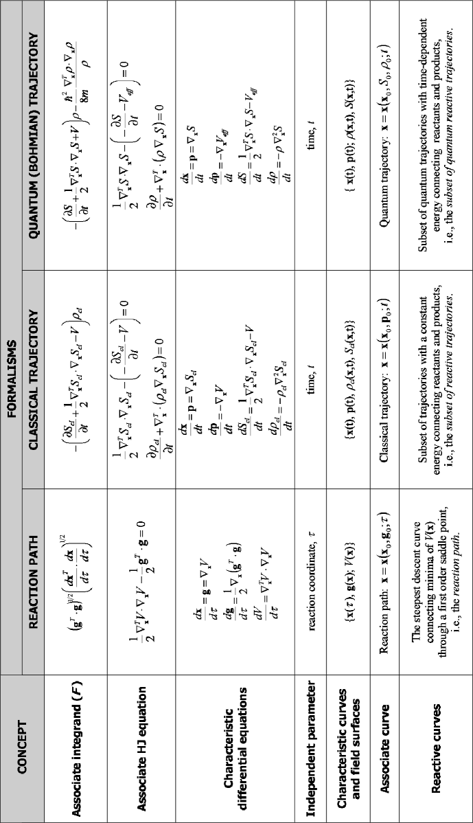
Figure 1: A schematic view of the generalized HJ framework presented in this work.

The generalized formulation discussed here is summarized in Fig. 1. As seen, mathematically RPs and classical/quantum trajectories are both characteristics coming from similar differential equations. However, important differences arise when the terms of the corresponding equations are identified. Thus, for a given PES, the RP follows a unique geodesic, steepest-descent curve, while there is an infinite set of classical/quantum trajectories solutions of the same differential equation (10)/(19), each one for an initial condition. Nonetheless, there is a common point: if one computes a set of steepest-descent curves for some given initial conditions ${\bf x}_{0}$ and ${\bf g}_{0}$, one fully ‘builds’ the PES. Similarly, from the set of classical trajectories for some given initial conditions $E$ and ${\bf x}_{0}$, one will then ‘build’ the action hypersurface $S_{cl}({\bf x},t)$ (the same for quantum trajectories). Formally, all the characteristics are obtained as solutions of (3), i.e., Eqs. (6), (10) and (19), which present similar functional forms. However, while $\tau$ represents the RP reaction coordinate and for each $\tau$ we have different values of the PES, it plays the role of time for a dynamical (classical or quantum) trajectory, which means that at every time we have a different value of the action hypersurface.

III Numerical simulations

III.1 The model

As a working model, we consider the Müller-Brown PES muellerbrown , which describes the reactants-to-products passage through an intermediate (pre-equilibrium) state,

$$R\rightleftharpoons I\rightharpoonup P.$$ (20)

This PES has three minima, $M_{1}(-0.558,1.442)$, $M_{2}(-0.050,0.467)$ and $M_{3}(0.623,0.028)$ (within this work, all magnitudes are given in atomic units), which describe the products, intermediate and reactants states, respectively. It has also two transition states, $TS_{1}(-0.822,0.624)$ and $TS_{2}(0.212,0.293)$, which separate products from pre-equilibrium and the latter from reactants, respectively. All these energies are indicated in Fig. 2a along the RP, which is described in terms of the arc-length

$$s(x,y)\approx\sum_{i=1}^{N}\sqrt{\Delta x_{i}^{2}+\Delta y_{i}^{2}}=\sum_{i=1}^{N}\sqrt{(x_{i}-x_{i-1})^{2}+(y_{i}-y_{i-1})^{2}},$$ (21)

where $(x_{0},y_{0})=M_{3}$, $(x_{N},y_{N})=(x,y)$, and the final point of the RP is $M_{1}$. Red circles represent the energies associated with minima ($V_{M_{1}}=-0.147$, $V_{M_{2}}=-0.081$ and $V_{M_{3}}=-0.108$) and blue ones with maxima ($V_{TS_{1}}=-0.041$ and $V_{TS_{2}}=-0.072$). A contour-plot of the Müller-Brown PES with the RP (green line) is displayed in the inset.

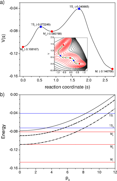
Figure 2: (a) Transition state energies ($TS$; blue circles) and reactants, pre-equilibrium and products energies ($M$; red circles) along the RP for the Müller-Brown PES. In the inset, a contour-plot of this PES with the RP (green line); black/red contours represent positive/negative equipotential contours. (b) Energy diagram as a function of the initial momentum (see text for details).

Regarding the dynamics, we have considered an initial Gaussian wave packet,

$$\Psi_{0}(x,y)=A_{0}\ \!e^{-(x-x_{0})^{2}/4\sigma_{x}^{2}-(y-y_{0})^{2}/4\sigma_{y}^{2}+ip_{x,0}(x-x_{0})/\hbar+ip_{y,0}(y-y_{0})/\hbar},$$ (22)

where $A_{0}=(2\pi\sigma_{x}\sigma_{y})^{-1/2}$, with $\sigma_{x}^{2}=\sigma_{y}^{2}=\sigma_{0}^{2}=0.0125$. This wave packet describes a proton transfer process and, hence, $m=1,836$ in the Schrödinger and Bohmian motion equations. In all calculations, the initial position of the wave-packet center is kept fixed at $(x_{0},y_{0})=M_{3}$, and only its initial momentum, chosen in all cases as $(p_{x,0},p_{y,0})=(-p_{0},p_{0})$, has been varied (indeed, the value of $p_{0}$). The initial conditions for the quantum trajectories are obtained randomly by sampling $\rho_{0}=|\Psi_{0}|^{2}\delta(p_{x}-p_{x,0})\delta(p_{y}-p_{y,0})$, while for classical trajectories we consider this distribution as well as the Wigner one associated with (22),

$$\rho_{W}(x,p_{x};y,p_{y})\propto e^{-(x-x_{0})^{2}/2\sigma_{x}^{2}-\sigma_{x}^{2}(p_{x}-p_{x,0})^{2}/\hbar^{2}-(y-y_{0})^{2}/2\sigma_{y}^{2}-\sigma_{y}^{2}(p_{y}-p_{y,0})^{2}/\hbar^{2}}.$$ (23)

Fig. 2b shows an energy diagram as a function of $p_{0}$, useful to understand the role played by the choice of initial momenta in classical/quantum trajectory simulations and, therefore, in the calculation of reaction probabilities (see Sec. III.2). In this diagram, the energy of the transition states and minima are indicated by color horizontal lines (blue and red, respectively). The black solid line represents the quantum expectation or average value of the energy, $\bar{E}=\langle\hat{H}\rangle$, which coincides with the classical average energy when the (classical) initial positions and momenta are chosen according to (23), since

$$\bar{E}=\int E(x,p_{x};y,p_{y})\rho_{W}(x,p_{x};y,p_{y})dxdydp_{x}dp_{y}=\frac{p_{0}^{2}}{m}+\bar{V}+\bar{\delta}\approx\frac{1}{N}\sum_{i=1}^{N}E_{i}(x_{0}^{i},y_{0}^{i}),$$ (24)

where $\bar{V}=\sum_{i=1}^{N}V_{i}(x_{0}^{i},y_{0}^{i})/N$, $\bar{\delta}=\hbar^{2}/4m\sigma^{2}$ is the spreading ratio sanz-jpa , and the last sum runs over all (classical/quantum) particles considered (with ($x_{0}^{i},y_{0}^{i}$) denoting their corresponding initial positions). The black dashed line is (24), but without $\bar{\delta}$, which coincides with a classical ensemble distributed initially according to $\rho_{0}$. In classical mechanics, the spreading ratio can be, therefore, related to the initial momentum distribution around $(p_{x,0},p_{y,0})$. Finally, the black dash-dotted line gives the energy of a classical particle initially located at $M_{3}$ and with initial momentum $(-p_{0},p_{0})$.

III.2 Trajectory ensemble analysis of reaction probabilities

The analysis of reaction probabilities can be carried out by defining the reaction probability in terms of the restricted norm sanz-jcp-sars

$$\mathcal{P}(t)\equiv\int_{\Sigma}|\Psi(x,y,t)|^{2}dxdy,$$ (25)

where $\Sigma$ denotes the space region above the line $y_{R\to P}(x)=0.8024x+1.2734$, here chosen as the frontier line separating products from the pre-equilibrium/reactants region (more refined choices could be considered, but no significant discrepancies are expected regarding products formation at this level). Apart from the amount of products in time, the initial slope of this function also provides information about the reaction velocity.

From a Bohmian viewpoint, (25) reads as the number of trajectories $N_{\Sigma}$ penetrating into $\Sigma$ at a time $t$ with respect to the total number $N$ of trajectories initially considered sanz-jcp-sars ,

$$\mathcal{W}(t)\equiv\frac{N_{\Sigma}(t)}{N},$$ (26)

which approaches $\mathcal{P}(t)$ when $N\to\infty$ and the initial conditions are sampled according to $\rho_{0}$. Classically, (26) can also be applied, but $\mathcal{W}_{\rm cl}(t)$ meaning a classical products fraction. Probability can flow backwards from products to reactants MC-W1 , which may lead to a multiple crossing of $y_{R\to P}(x)$ by the same quantum/classical trajectory. Hence, another interesting quantity is the fraction of trajectories going from reactants to products without taking into account their return to reactants,

$$\bar{\mathcal{W}}(t)\equiv\frac{\bar{N}_{\Sigma}(t)}{N},$$ (27)

which, at $t\to\infty$, provides the total amount of products for a given initial state. That is, assuming that one could extract the products formed during the reaction by some chemical or physical procedure, $\bar{\mathcal{W}}(t)$ would provide the maximum amount of products. Note that this information is only available when working with trajectories, since one can visualize each individual process and, therefore, detect when one reactive event has taken place.

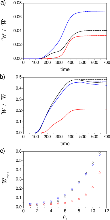
Figure 3: Reaction probabilities $\mathcal{W}$ (solid curve) and $\bar{\mathcal{W}}$ (dashed curve) for: (a) $p_{0}=4$ and (b) $p_{0}=10$, and three different initial distributions: quantum trajectories distributed according to $\rho_{0}$ (black) and classical trajectories distributed according to $\rho_{0}$ (red) and $\rho_{W}$ (blue). In panel (c), $\bar{\mathcal{W}}$ at $t\approx 700$ as a function of $p_{0}$: black circles denote $\bar{\mathcal{W}}_{\rm Bohm}$, red triangles, $\bar{\mathcal{W}}_{\rm Bohm}^{\rm cl}$, and blue inverted triangles, $\bar{\mathcal{W}}_{\rm Wigner}^{\rm cl}$.

In Figs. 3(a) and 3(b), we have plotted $\mathcal{W}$ (solid line) and $\bar{\mathcal{W}}$ (dashed line) for $p_{0}=4$ and $p_{0}=10$, respectively, and three different initial distributions: quantum trajectories distributed according to $\rho_{0}$ (black) and classical trajectories distributed according to $\rho_{0}$ (red) and $\rho_{W}$ (blue). Results from (25) have not been plotted since they are identical to those obtained from (26). In all cases, a total of $5\times 10^{4}$ trajectories has been considered and a propagation up to $t=700$, the asymptotic value at which $\bar{\mathcal{W}}$ stabilizes. As seen in Fig. 2b, for $p_{0}=4$, $\bar{E}-\bar{\delta}$ (dashed curve) is well below $TS_{2}$ and $TS_{1}$. Therefore, according to standard quantum mechanics, the actual dynamics in Fig. 3a should then proceed mainly via tunneling. We clearly observe that $\mathcal{W}_{\rm Bohm}$ is below $\mathcal{W}_{\rm Wigner}^{\rm cl}$ and closer to $\mathcal{W}_{\rm Bohm}^{\rm cl}$. This can be explained as follows. The classical distributions explore many initial conditions, which eventually may imply individual trajectory energies higher than the transitions states and therefore lead to the formation of products. This effect is more striking in the case of the Wigner distribution than in the classical Bohmian one, where the initial momentum is fixed. On the other hand, for Bohmian trajectories the dynamics is radically different: for low $p_{0}$, the wave packet spreads faster than it moves and, hence, the expected formation of ripples by interference is going to hinder the passage of Bohmian trajectories to products. Note that in Bohmian mechanics tunneling does not exist as it is commonly understood in standard quantum mechanics, but as an effect arising from the modification in time of the barrier due to the quantum potential; a time-dependent, effective barrier, given by (18), is what actually rules the trajectory dynamics. For $p_{0}=10$, however, $\bar{E}-\bar{\delta}$ is above $TS_{1}$ in Fig. 2b, which suggests (quantum-mechanically) a larger amount of products by direct passage rather than tunneling. This will cause that the classical Wigner distribution and the (quantum) Bohmian one will render much closer results, as it is observed in Fig. 3b, where $\mathcal{W}_{\rm Bohm}$ approaches $\mathcal{W}_{\rm Wigner}^{\rm cl}$, but is far from $\mathcal{W}_{\rm Bohm}^{\rm cl}$. In this case, though tunneling can still be active, the direct passage is going to control the dynamics in both cases, classical and quantum-mechanical. Observe that, in the second case, the translational motion is faster than the spreading of the wave packet and, therefore, more trajectories can be promoted to products before interference starts to influence the trajectory dynamics. Regarding $\bar{\mathcal{W}}$, we find a trend similar to $\mathcal{W}$, but the difference between the asymptotic values of these magnitudes increases with $p_{0}$, which is due to the larger amount of energy available and therefore the increase of recrossings (for the classical Bohmian distribution the effect is negligible, because of the less energy available after fixing $p_{0}$).

In Fig. 3c, the maximum amount of products, $\bar{\mathcal{W}}$, is plotted as a function of $p_{0}$ for the same distributions as above. As can be noticed, the formation of products is more efficient classically than quantum-mechanically until relatively large values of $p_{0}$; indeed, both classical distributions provide a larger amount of products for $p_{0}\lesssim 4$. As noticed in Fig. 2b, $\bar{E}$ crosses $TS_{2}$ at $p_{0}\approx 3.5$; in Fig. 3c, after this $p_{0}$ value, the Bohmian distribution provides larger reaction probabilities than its classical counterpart, the difference between them increasing with $p_{0}$. As $p_{0}$ is further increased, the Bohmian and Wigner distributions start to get closer, though the latter gives rise to a larger probability until $p_{0}\sim 8$-9, where the situation is reversed. Again, this coincides with $\bar{E}$ crossing a transition state, this time the one connecting the pre-equilibrium with products.

Summarizing, though an ensemble magnitude may have very similar values classically and quantum-mechanically, the underlying dynamics can be radically different, which arises from both the effects of the quantum potential and the mathematical structure of the corresponding motion equations (see Sec. II): in Bohmian mechanics the momentum readjusts at each instant in order to satisfy the statistical requirements of quantum mechanics, while in classical mechanics positions and momenta are not coupled. Next, we analyze in more detail the underlying dynamics in terms of common elements within the generalized HJ framework: RPs and classical/quantum trajectories.

III.3 Quantum-classical trajectory analysis

As seen in Fig. 2b, values of $p_{0}$ between 8 and 10 are critical, since the dynamics is developed around the $TS_{1}$ from the pre-equilibrium region. Thus, in Fig. 4, two pairs of trajectories for $p_{0}=9$ have been purposely chosen. In each panel, both members of the pair start exactly with the same initial conditions. However, in (a) the quantum trajectory (green) is reactive through two-dimensional tunneling, while its classical partner (blue) is inelastic, whereas in (b) both trajectories are inelastic. The different and richer behaviors displayed by quantum trajectories are due to their motion being ruled by the quantum potential (apart from the PES), which is lacking in classical dynamics.

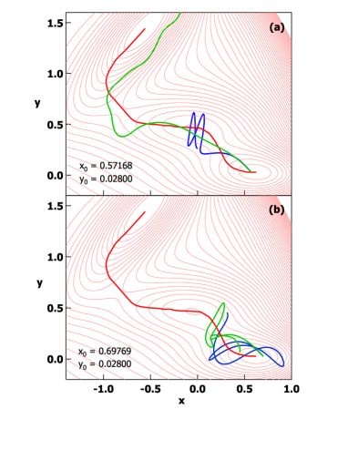
Figure 4: Classical (blue) and quantum (green) trajectories representative of the dynamics on a Müller-Brown PES (in red, the RP): (a) the quantum trajectory is reactive through two-dimensional tunneling, while its classical counterpart is inelastic; (b) both trajectories are inelastic. The classical and quantum trajectories are launched from the initial positions indicated at the lower left corner of each respective panel and with the same initial momentum, $p_{0}=9$.

In order to better understand these behaviors, we consider differences $\Delta A(t)=A_{q}(t)-A_{cl}(t)$, where $A_{q}(t)$ and $A_{cl}(t)$ denote the quantum magnitude and its classical counterpart, respectively. Thus, in Fig. 5, we show the differences in positions ($\Delta x$ and $\Delta y$) and momenta ($\Delta p_{x}$ and $\Delta p_{y}$) for the pairs of trajectories displayed in Fig. 4 up to the time when one member of the pair approaches the first saddle point ($t\approx 100$ a.u.). Moreover, the total energy, computed from the classical-like expression

$$E(t)=\frac{p_{x}^{2}(t)}{2m}+\frac{p_{y}^{2}(t)}{2m}+V(x(t),y(t)),$$ (28)

is also plotted along each classical (thinner)/quantum (thicker) trajectory (blue lines) taking into account the energy scale in the right vertical axes of both panels of the corresponding figure. At $t=0$, (28) is between $V_{TS_{2}}$ and $V_{TS_{1}}$ (see Fig. 2b) for both classical trajectories and, therefore, none of them will be able to overcome the barrier leading to products at any subsequent time since, classically, the energy conserves. Hence, they will remain wandering within the reactants and pre-equilibrium regions. Regarding the quantum dynamics, the trajectory in Fig. 4a basically follows the RP, thus reaching the products region. When compared with its classical counterpart, we note that, at the earlier stages of its time evolution, the separation of both types of trajectories is increasing. This fact suggests that the quantum trajectory is visiting a wider region of phase space than the corresponding classical one (termed as dynamical tunneling by Heller heller ), even before reaching the potential barrier (barrier tunneling). Thus we could say that we have a double contribution to tunneling. The main contribution to the reaction probability will come from the dynamical tunneling since, in two or higher dimensions, the trajectory can skip the barrier very easily by exploring new regions of phase space. On the contrary, the quantum trajectory of Fig. 4b is inelastic because there is no route to products mediated by tunneling. Arguing in topological terms, this trajectory is launched pointing towards a part of the PES with a stronger gradient (i.e., a more repulsive wall); the trajectory is not capable then to overcome the increasing bending and go backwards, so it remains trapped at the pre-equilibrium region. This dynamical picture of tunneling in two dimensions thus seems to be more demanding than in one dimension, since not only energy criteria, but also the initial momentum orientation should be taken into account.

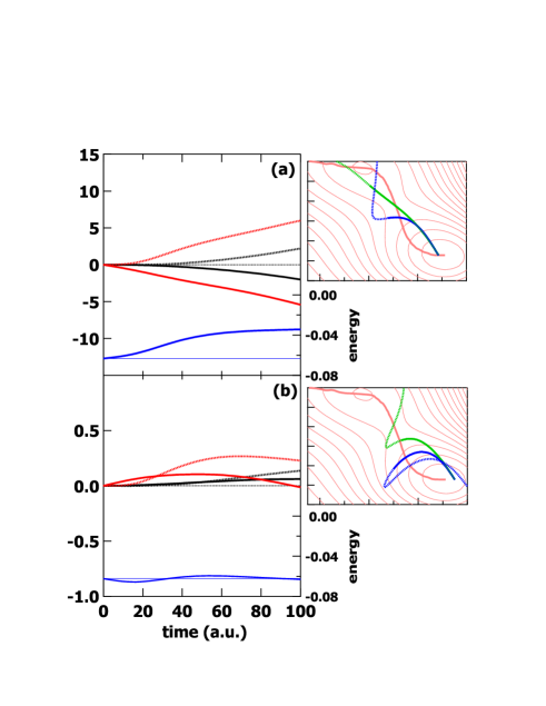
Figure 5: Quantum-classical differences for the pairs of trajectories displayed in Figs. 4(a) and 4(b): $\Delta x(t)$ (black solid), $\Delta y(t)$ (black dashed), $\Delta p_{x}(t)$ (red solid) and $\Delta p_{y}(t)$ (red dashed). The total energy (28) is also displayed (the scale is on the right side of each panel), with blue thinner/thicker line for classical/quantum trajectories (the classical energy is constant with time). In the aside plots, solid lines indicate the portion of the trajectories up to the time when one member of the pair approaches the first saddle point ($t\approx 100$ a.u.).

Energetically, quantum dynamics look so different from classical ones (for instance, we may observe reactivity quantum-mechanically, but not classically, as mentioned above) because (28) does not conserve along quantum trajectories. This can be appreciated in Fig. 5, when comparing the value of this magnitude for the two quantum trajectories along time. In Fig. 5a, there is a relatively fast initial expansion or ‘boost’ wyatt1 ; wyatt2 which leads to an increase of the energy and therefore enhances the possibility of tunneling though the initial energy was smaller than the barrier height. On the contrary, the second trajectory does not benefit from this expansion (its energy remains nearly conserved) and, therefore, no tunneling is expected.

III.4 Statics-dynamics analysis

Finally, we would like to provide some clues aimed to clarify the long-standing static-dynamic controversy, i.e., whether statics suffices to establish reaction mechanisms or, on the contrary, true reaction mechanisms are very different from the information provided by statics and, therefore, dynamics is compulsory. A direct approach to tackle this problem consists of studying the differences in configuration space between the RP and classical/quantum trajectories. In principle, any static-dynamic comparison might be hampered by the different physical meaning of the independent parameter characterizing each curve as well as the dimensionality of the problem. In order to avoid these difficulties, though at the expense of losing some dynamical details, one can consider projection schemes. For instance, trying to check the accuracy of the RP formalism, Taketsugu and Gordon gordon tackled such a problem using two distances, the perpendicular and the distance of closest approach. We propose a generalization of this approach by computing the whole set of distances between the RP and a given trajectory. This generates a matrix with elements

$$C_{ij}=|{\bf x}(t_{i})-{\bf x}_{\rm RP}(s_{j})|^{2},$$ (29)

where the $(i,j)$-element gives the distance between a (classical or quantum) trajectory, ${\bf x}(t_{i})$, at a time $t_{i}$, and the RP ${\bf x}_{\rm RP}(s_{j})$, at a value $s_{j}$ of the reaction coordinate (of course, the same division in segments is assumed for the trajectory and the RP), and whose visual display gives rise to the so-called Carathéodory plot cara . These plots have the property that they are always three-dimensional surfaces regardless of the number of degrees of freedom of the problem because they are based on the definition of distance (29). In Fig. 6, we present the Carathéodory plots associated with the quantum trajectories displayed in Figs. 4(a) and 4(b). The quantum trajectory of Fig. 4a is able to tunnel across the highest TS and reach the products region keeping its kinetic energy considerably lower than that of classical reactive trajectories. Hence, it remains reasonably close to the RP rather than oscillating around it (as it might be expected classically), this leading to a Carathéodory plot which displays a valley essentially along its diagonal (see Fig. 6a). On the contrary, the quantum trajectory in Fig. 4b is inelastic and, therefore, departs remarkably from the RP, this giving rise to a minimum valley out of the diagonal (see Fig. 6b).

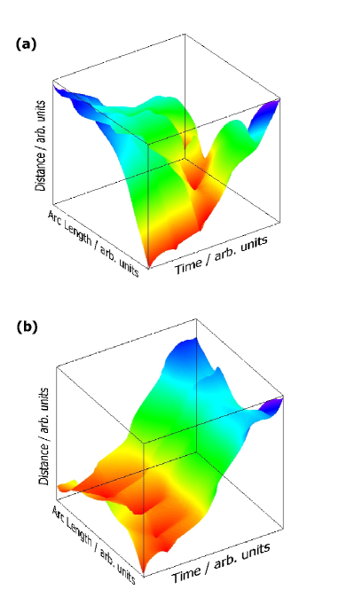
Figure 6: In panels (a) and (b), Carathéodory plots associated with the quantum trajectories displayed in Figs. 4(a) and 4(b), respectively. The transition from red to blue indicates an increasing distance between the RP and the respective quantum trajectory.

IV Conclusions

Here, we have shown the guidelines to carry out analyses of molecular reactions within a generalized HJ framework, which allows to encompass both topology and classical/quantum dynamics: static RPs arise when a variational kernel is associated with a PES gradient, whereas classical/quantum trajectories are obtained when it corresponds to properly defined classical/quantum Lagrangians. Specifically, the application of this scheme to the topology and dynamics in a Müller-Brown PES has shown outstanding features, such as a better understanding of the discrepancies found between classical and quantum statistical results. For instance, reaction probabilities have been computed with Bohmian and Wigner distributions of initial conditions. As seen, though both rates look pretty close for some values of $p_{0}$, their corresponding underlying dynamics are dramatically different because of the quantum-mechanical coupling between individual trajectories and their distribution. This leads to dynamics totally different from their classical analogs and, therefore, to effects not observable classically, such as dynamical tunneling. It is also worth stressing that computing $\bar{\mathcal{W}}$ and displaying its asymptotic value as a function of $p_{0}$ (or another parameter characterizing the initial state), can be of interest from an experimental viewpoint, for it constitutes a simple method to determine the maximum amount of products formed during a reaction. Since $\bar{\mathcal{W}}_{\rm max}$ provides an upper bound for the reaction probability, it could be used to establish some control mechanism on the reaction based on modifying one parameter in the initial state preparation (here, $p_{0}$, which could be varied by using laser pumping techniques, for instance). On the other hand, quantum-classical differences, obtained from a one-to-one comparison of classical and quantum trajectories with the same initial conditions, give evidence of dynamical tunneling at early time evolution stages, this contribution being mainly the responsible for the occurrence of reaction at certain initial conditions. Barrier tunneling is expected to be very small. Finally, the construction of Carathéodory plots has been shown to be an interesting tool to analyze static-dynamic differences (i.e., between RPs and classical/quantum trajectories). Depending on whether the trajectory is reactive or not, these plots show distinct topographical shapes: tunneling reactive trajectories lead to diagonally dominated valleys, whereas inelastic, non-reactive ones lead to a much more involved shape. Furthermore, since these plots do not depend on the problem dimensionality, they could result advantageous to analyze processes involving large molecules.

- (1) See, for instance: Faraday Discuss. Chem. Soc. 110 (1998).
- (2) K. Fukui, J. Phys. Chem. 74 (1970) 4161.
- (3) A. Aguilar-Mogas, X. Giménez, J.M. Bofill, J. Chem. Phys. 128 (2008) 104102.
- (4) J.H. van Vleck, Proc. Natl. Acad. Sci. US 14 (1928) 178.
- (5) R. Schiller, Phys. Rev. 125 (1962) 1100.
- (6) R. Schiller, Phys. Rev. 125 (1962) 1109.
- (7) W.H. Miller, Proc. Nat. Acad. Sci. 102 (2005) 6660.
- (8) W.H. Miller, J. Chem. Phys. 125 (2006) 132305.
- (9) J.G. Muga, R. Sala, R.F. Snider, Phys. Scr. 47 (1993) 732.
- (10) J.P. Palao, J.G. Muga, C.R. Leavens, Phys. Lett. A 253 (1999) 21.
- (11) E. Madelung, Z. Phys. 40 (1926) 322.
- (12) E.A. McCullough, R.E. Wyatt, J. Chem. Phys. 51 (1969) 1253.
- (13) E.A. McCullough, R.E. Wyatt, J. Chem. Phys. 54 (1971) 3578.
- (14) E.A. McCullough, R.E. Wyatt, J. Chem. Phys. 54 (1971) 3592.
- (15) D. Bohm, Phys. Rev. 85 (1952) 166.
- (16) P.R. Holland, The Quantum Theory of Motion, Cambridge University Press, Cambridge, 1993.
- (17) R.E. Wyatt, Quantum Dynamics with Trajectories, Springer, New York, 2005.
- (18) C.L. Lopreore, R.E. Wyatt, Phys. Rev. Lett. 82 (1999) 5190.
- (19) C.L. Lopreore, R.E. Wyatt, Chem. Phys. Lett. 325 (2000) 73.
- (20) R. Guantes, A.S. Sanz, J. Margalef-Roig, S. Miret-Artés, Surf. Sci. Rep. 53 (2004) 199.
- (21) A.S. Sanz, S. Miret-Artés, Phys. Rep. 451 (2007) 37.
- (22) M.F. González, X. Giménez, J. González-Aguilar, J.M. Bofill, J. Phys. Chem. A 111 (2007) 10226.
- (23) K. Müller, L.D. Brown, Theor. Chim. Acta 53 (1979) 75.
- (24) J. González, X. Giménez, J.M. Bofill, Phys. Chem. Chem. Phys. 4 (2002) 2921.
- (25) N. Isaacs, Physical Organic Chemistry, Longman Scientific & Technical, London, 1995 (2nd ed.).
- (26) C. Carathéodory, Calculus of Variations and Partial Differential Equations of the First Order, Chelsea Publishing Company, New York, 1982.
- (27) R. Crehuet, J.M. Bofill, J. Chem. Phys. 122 (2005) 234105.
- (28) D. Heidrich (ed.), The Reaction Path in Chemistry: Current Approaches and Perspectives, Kluwer, Dordrecht, 1995.
- (29) H.B. Schlegel, J. Comp. Chem. 24 (2003) 1415.
- (30) R. Courant, D. Hilbert, Methods in Mathematical Physics, Wiley, New York, 1953.
- (31) M. Born, E. Wolf, Principles of Optics, Cambridge University Press, Cambridge, 1999 (7th ed.).
- (32) W. Quapp, Theor. Chem. Account. 121 (2008) 227.
- (33) L.D. Landau, E.M. Lifshitz, The Classical Theory of Fields, Butterworth Heinemann, Amsterdam, 1947.
- (34) H. Goldstein, Classical Mechanics, Addison-Wesley, Reading, MA, 1980.
- (35) T. Takabayasi, Prog. Theor. Phys. 8 (1952) 143.
- (36) A.S. Sanz, S. Miret-Artés, J. Phys. A 41 (2008) 435303.
- (37) A.S. Sanz, S. Miret-Artés, J. Chem. Phys. 122 (2005) 014702.
- (38) E.J. Heller, J. Phys. Chem. A 103 (1999) 10433.
- (39) T. Taketsugu, M.S. Gordon, J. Chem. Phys. 103 (1995) 10042.