Tree Orbits under Permutation Group Action: Algorithm, Enumeration and Application to Viral Assembly

Abstract

This paper uses combinatorics and group theory to answer questions about the assembly of icosahedral viral shells. Although the geometric structure of the capsid (shell) is fairly well understood in terms of its constituent subunits, the assembly process is not. For the purpose of this paper, the capsid is modeled by a polyhedron whose facets represent the monomers. The assembly process is modeled by a rooted tree, the leaves representing the facets of the polyhedron, the root representing the assembled polyhedron, and the internal vertices representing intermediate stages of assembly (subsets of facets). Besides its virological motivation, the enumeration of orbits of trees under the action of a finite group is of independent mathematical interest. If $G$ is a finite group acting on a finite set $X$, then there is a natural induced action of $G$ on the set $\mathcal{T}_{X}$ of trees whose leaves are bijectively labeled by the elements of $X$. If $G$ acts simply on $X$, then $|X|:=|X_{n}|=n\cdot|G|$, where $n$ is the number of $G$-orbits in $X$. The basic combinatorial results in this paper are (1) a formula for the number of orbits of each size in the action of $G$ on $\mathcal{T}_{X_{n}}$, for every $n$, and (2) a simple algorithm to find the stabilizer of a tree $\tau\in\mathcal{T}_{X}$ in $G$ that runs in linear time and does not need memory in addition to its input tree.

2000 Mathematics Subject Classification: Primary 05C05, 05A15, 20B25, 92C50.

Key words: tree enumeration, generating function, group action, viral capsid assembly.

1 Introduction

Viral shells, called capsids, encapsulate and protect the fragile nucleic acid genome from physical, chemical, and enzymatic damage. Francis Crick and James Watson (1956) were the first to suggest that viral shells are composed of numerous identical protein subunits called monomers. For many viruses, these monomers are arranged in either a helical or an icosahedral structure. We are interested in those shells that possess icosahedral symmetry.

Icosahedral viral shells can be classified based on their polyhedral structure, facets corresponding to the monomers. The classical “quasi-equivalence theory” of Caspar and Klug [6] explains the structure of the polyhedral shell in the case where the monomers have very similar neighborhoods. According to the theory, the number of facets in the polyhedron is $60T$, where the $T$-number is of the form $h^{2}+hk+k^{2}$. Here $h$ and $k$ are non-negative integers. The icosahedral group acts simply on the set of facets of the polyhedron (monomers of the shell).

Although for many virus families the structure is fairly well understood and substantiated by crystallographic images, the viral assembly process - just like many other spontaneous macromolecular assembly processes - is not well-understood, even for $T=1$ viral shells. In many cases, the capsid self-assembles spontaneously, rapidly and quite accurately in the host cell, with or without enclosing the internal genomic material, and without the use of chaperone, scaffolding or other helper proteins. This is the type of assembly that we consider here. See Figure 1 for basic icosahedral structure and X-ray structure of a T=1 virus.

,

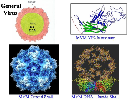
Figure 1: (Left) Basic Viral Structure. (Right) Minute virus of Mice X-ray and monomer structure courtesy [1]

.

Many mathematical models of viral shell assembly have been proposed and studied including [2, 4, 12, 14, 15, 16, 25, 26, 27]. Here we use the GT (geometry and tensegrity) model of [18]. In the GT model, information about the construction (or decomposition) of the viral shell is represented by an assembly tree. The vertices of the tree represent subassemblies that do not disintegrate during the course of the assembly process. In an assembly tree, these subassemblies are partially ordered by containment, with the root representing the complete assembled structure, and the leaves representing the monomers. That is, we only consider trees that represent successful assemblies. See Figure 2 for the nomenclature of a $T=1$ polyhedron, and Figures 3, 4 for examples of assembly trees. Besides being intuitive and analyzable, it was shown in [18] that the GT model’s rough predictions fit experimental and biophysical observations of known $T=1$ viral assemblies, specifically those of the viruses MVM (Minute Virus of Mice), MSV (Maize Streak Virus) and AAV4 (Human Adeno Associate Virus).

The GT model was developed to answer questions that concern only the influence of two quantities on the probability of each type of assembly tree. We call these quantities the geometric stability factor and the symmetry factor. The higher these quantities, the higher the probability.

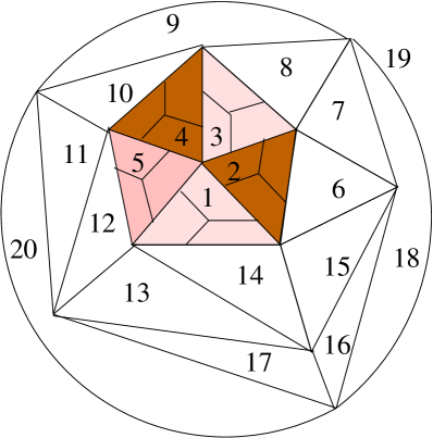
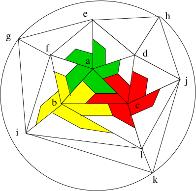
Figure 2: (Left) Face numbers: pentamer of trimers in a $T=1$ polyhedron. (Right) Vertex numbers: trimers of pentamers in a $T=1$ polyhedron.

The geometric stability factor is correlated with biochemical stability and influenced by assembly and disassembly energy thresholds and is defined using the effect of geometric constraints within monomers or between monomers. These constraints are distances, angles and forces between the monomer residues. These can be obtained either from X-ray or from cryo-electro-microscopic information on the complete viral shell. More specifically, the final viral structure can be viewed formally as the solution to a system of geometric constraints that can be expressed as algebraic equations and inequalities. For each internal vertex of an assembly tree, namely a subassembly, the geometric stability factor can be computed using quantifiable properties - such as extent of rigidity or algebraic complexity of the configuration space of the subassembly.

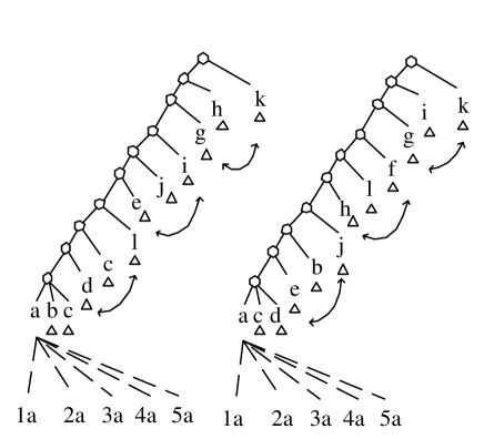
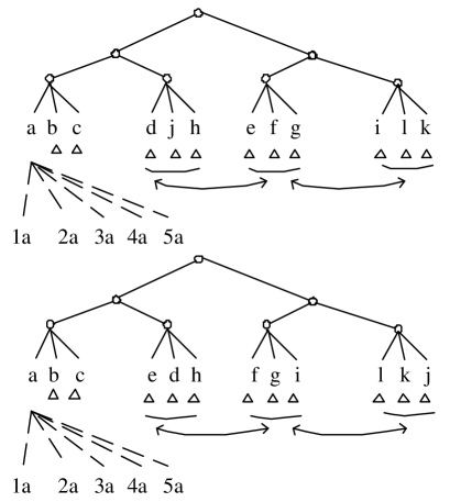
Figure 3: $T=1$ valid assembly trees based on pentameric subassemblies and nomenclature of Figure 2, triangles at bottom represent vertices with five leaves as children; arrows represent the action of the icosahedral group on trees ; only the long horizontal arrows in the two figures on right fix the corresponding trees.

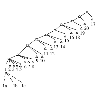
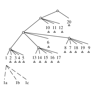
Figure 4: $T=1$ valid assembly trees based on trimeric subassemblies, triangles at bottom represent trimers.

This factor is computed by analyzing the corresponding subsystems of the given viral geometric constraint system. It was argued in [18] that the rigidity aspect of the geometric stability factor can be generically expressed purely using graph theory. Some assembly trees can never occur (have probability zero) since the subassemblies occurring in them are unstable (their geometric stability factor is zero). Such assembly trees are geometrically invalid.

The symmetry factor is defined as follows. The icosahedral group acts naturally on the set of assembly trees for a particular viral polyhedron $P$, whose facets (representing viral monomers) are the leaves of the tree as illustrated in Figure 3. Each orbit under this action is called an assembly pathway and corresponds intuitively to a distinct type of assembly process for the viral capsid. The symmetry factor is the number of assembly trees in the pathway divided by the total number of trees. We assume that each assembly tree is equally likely to occur.

In [19], the authors observed the following attractive feature of the GT model of assembly. The two separate factors - geometric stability and symmetry - that influence the probability of the occurrence of a particular assembly pathway can be analyzed largely independently as follows. An obvious, but crucial, observation made in [19] is that both the geometric stability factor and geometric validity are invariants of the assembly pathway. That is, they remain the same for any assembly tree in the same orbit under the action of the icosahedral group. Thus the probability of the occurrence of a pathway is roughly proportional to some combination of the symmetric factor and the geometric stability factor. Additionally, the ratio of the orbit sizes of two trees $\tau_{1}$ and $\tau_{2}$ could serve as a rough estimate of the the ratio of the probabilities of the corresponding assembly pathways - provided that the former ratio is not cancelled out or reversed by the ratio of the geometric stability factor of $\tau_{1}$ and $\tau_{2}$. The paper [3] formally proved that this kind of cancelling out would not generally take place, at least for valid pathways, for the following reasons. First, it is shown in [3] that the symmetry factor of a pathway increases with the depth of its representative tree $\tau$. More precisely, it was proved formally that the size of the orbit of $\tau$ is bounded below by the depth of $\tau$. Moreover, it is known from [18] that, provided an assembly tree is valid, the geometric stability factor is non-zero and generally increases with the depth of the tree (and this correlates with biophysical observations). Therefore, if the depth of $\tau_{1}$ is greater than the depth of $\tau_{2}$, then both the symmetric factor and the geometric stability factor of $\tau_{1}$ will generally be larger than the corresponding factors of $\tau_{2}$.

1.1 Contributions and Related Work

Based on the observations in the last section, the paper [3] posed problems intended to isolate and clarify the influence of the symmetry factor on the probability of the occurrence of a given assembly pathway. Two specific problems were the following.

1. Enumerate the valid assembly pathways of an icosahedrally symmetric polyhedron. More precisely, the problem is to determine the number of such assembly pathways of each orbit size.

2. Characterize and algorithmically recognize the set of assembly trees fixed by a given subgroup of the icosahedral group. The characterization problem is a step toward the solution of the enumeration problem (i). Algorithmic recognition of the group elements that fix a given assembly tree (the stabilizer of the tree in the given group) directly determines whether the given assembly tree has a given orbit size.

Remark. In this paper, we answer the above questions for general assembly trees, that is, we drop the condition of validity. Furthermore, in this paper, the geometric stability factor will be ignored, and thus “probability” will refer to tbe symmetry factor only. As mentioned earlier, [18, 19] show that validity of assembly trees of a polyhedron $P$ is not only invariant under the action of its symmetry group, but can also be captured by simple graph-theoretic properties such as generalized notions of connectivity for the graph constructed from the vertices and edges of $P$. We expect that the techniques developed in this paper will help in answering the above questions in the presence of the validity condition as well.

For Problem (i), we develop an enumeration method using generating functions and Möbius inversion. For the algorithm in Problem (ii), we provide a simple permutation group algorithm and an associated data structure. The results of this paper work not just for the icosahedral group, but also for any finite group $G$ acting simply on a set $X$. Indeed, if $G$ is a finite group acting on a set $X$, then there is a natural induced action of $G$ on the set ${\mathcal{T}}_{X}$ of assembly trees. These are formally defined as rooted trees $\tau$ whose non-leaf vertices have at least two children and whose leaves are bijectively labeled by $X$. If $G$ acts simply on $X$, then $|X|:=|X_{n}|=n\,|G|$, where $n$ is the number of $G$-orbits in $X$.

Concerning Problem (i), Pólya theory gives a convenient method for counting orbits under a permutation group action. However, because of the complexity of the cycle index in our situation, we were not able to apply Pólya theory to Problem (i). Similarly, the methods used in [13] for enumerating labeled graphs under a group action (as opposed to rooted labeled trees), did not seem to apply. Our generating function method, on the other hand, finds an explicit formula (Theorem 3) for the number of orbits of each possible size in the action of $G$ on the set ${\mathcal{T}}_{X_{n}}$ of assembly trees, for every $n$. This leads to a formula for the probability of occurrence of a given assembly pathway (Corollary 5). To apply these formulas it is necessary to know the number of assembly trees fixed by each given subgroup of G. A generating function formula for this number of fixed assembly trees is given in Theorem 16 of Section 5. For the proof of Theorem 16 is is necessary to characterize the set of such fixed assembly trees. This is done in Theorem 9 of Section 4.

Concerning Problem (ii), algorithms for permutation groups have been well-studied (see for example [17]), and algorithms for tree isomorphism and automorphism are well known [8, 21]. Moreover, the structure of the automorphism groups of rooted, labeled trees have been studied [11, 23]. However, we have not encountered an algorithm in the literature for deciding whether a given permutation group element fixes a given rooted, labeled tree; and thereby finds the stabilizer of that tree in the given group $G$. In Section 3.2 of this paper, we provide a simple and intuitive algorithm that is easy to implement, runs in linear time and operates in place on the input, without the use of extra scratch memory.

If one is only interested in approximate and asymptotic estimates for Problem (i), such as in viruses with large T-numbers, a possible avenue is to use the results of [7, 24] that estimate the asymptotic probabilities of logic properties on finite structures, especially trees. There are significant roadblocks, however, to applying these results to our problem. These are mentioned in the open problem section at the end of this paper. Finally, there is a rich literature on the enumeration of construction sequences of symmetric polyhedra and their underlying graphs [5, 9, 10]. Whereas these studies focus on enumerating construction sequences of different polyhedra with a given number of facets, our goal - of counting and characterizing assembly tree orbits - is geared towards enumerating construction sequences of a single polyhedron for any given number of facets.

2 Preliminaries on Assembly Pathways

All groups, graphs, and label sets in this paper are assumed to be finite. A rooted tree is a tree with a designated vertex, called the root. We will use standard terminology such as adjacent, child, parent, descendent, ancestor, leaf, subtree rooted at, root of the subtree, and so on. For our purposes, a rooted tree is called a labeled tree if the leaves are bijectively labeled by the elements of a set $X$, and an internal (non-leaf) vertex $v$ is labeled by the set of leaf-labels of the subtree rooted at $v$. We identify each vertex in a tree with its label. Let $\tau$ and $\tau^{\prime}$ be two rooted trees labeled in the same set $X$. Then $\tau$ and $\tau^{\prime}$ are said to be isomorphic if there is a bijection - the isomorphism - $f$ between the vertices of $\tau$ and $\tau^{\prime}$ that preserves adjacency and the root. That is, all the following hold.

• $(u,v)$ is an edge in $\tau$ if and only if $(f(u),f(v))$ is an edge in $\tau^{\prime}$,

• $f(r)=r^{\prime}$, where $r$ and $r^{\prime}$ are the roots of $\tau$ and $\tau^{\prime}$ respectively In this case, we say $\tau\approx\tau^{\prime}$ and also $f(\tau)=\tau^{\prime}$.

An automorphism $f$ of $\tau$ is an isomorphism of $\tau$ into itself: it ensures that $(u,v)$ is an edge in $\tau$ if and only if $(f(u),f(v))$ is also an edge in $\tau$. In this case $f(\tau)=\tau$.

A rooted tree for which each internal vertex has at least two children and whose leaves are labeled with elements of $X$ is called an assembly tree for $X$. The $26$ assembly trees with four leaves, labeled in the set $X=\{1,2,3,4\}$ are shown in Figure 5.

Let $G$ be a group acting on a set $X$. The action of $G$ on $X$ induces a natural action of $G$ on the power set of $X$ and thereby on the set of vertices (vertex labels) of $\mathcal{T}_{X}$ of assembly trees for $X$. If $g\in G$ and $\tau\in\mathcal{T}_{X}$, then define the tree $g(\tau)$ as the unique assembly tree whose set of vertex labels (including the labels of internal vertices) is $\{g(v):v\in\tau\}$. This tree $g(\tau)$ is clearly isomorphic to $\tau$ via $g$. This induces an action of $G$ on $\mathcal{T}_{X}$. Each orbit of this action of $G$ on $\mathcal{T}_{X}$ consists of isomorphic trees and is called an assembly pathway for $(G,X)$.

Figure 5: Klein 4-group acting on $\mathcal{T}_{4}$.

Example 1

Klein 4-group acting on $\mathcal{T}_{4}$.

Consider the Klein 4-group $G={\mathbb{Z}}_{2}\oplus{\mathbb{Z}}_{2}$ acting on the set $X=\{1,2,3,4\}$. Writing $G$ as a group of permutations in cycle notation, this action is

$$G=\{(1)(2)(3)(4),\,(1\;2)(3\;4),\,(1\;3)(2\;4),\,(1\;4)(2\;3)\}.$$

For this example there are exactly 11 assembly pathways, which are indicated in Figure 5 by boxes around the orbits. There are four assembly pathways of size one, i.e., with one assembly tree in the orbit, three assembly pathways of size two, and four assembly pathways of size four.

An assembly tree $\tau$ is said to be fixed by an element $g\in G$ if $g$ is an automorphism of $\tau$, that is, $g(\tau)=\tau$. See Figure 3 for an illustration. For any subgroup $H$ of $G$, let $\overline{t}(H):=\overline{t_{X}}(H)$ denote the number of trees in $\mathcal{T}_{X}$ that are fixed by all elements of $H$ and by no other elements of $G$. In other words,

$$\overline{t}_{X}(H)=|\{\tau\in\mathcal{T}_{X}\,|\,stab_{G}(\tau)=H\}|.$$ (1 )

Here $stab_{G}(\tau):=\{g\in G\;|\;g(\tau)=\tau\}$ is called the stabilizer of $\tau$ in $G$. In other words, $stab_{G}(\tau)$ is the set of all elements in $G$ that fix $\tau$. It is easy to prove that $stab_{G}(\tau)$ is a subgroup of $G$.

In fact, we will see in Section 5 that it is more natural to find $t_{X}(H)$, i.e., the number of trees in $\mathcal{T}_{X}$ that are fixed by a subgroup $H$ of $G$. These may include trees that are fixed by larger subgroups $H^{\prime}$ such that $H\leq H^{\prime}\leq G$. As the following theorem shows, the desired quantities $\overline{t}_{X}(H)$ can then be computed from the numbers $t_{X}(H)$ using Möbius inversion on the lattice of subgroups of $G$.

Theorem 2

Let $G$ be a group acting on a set $X$. If $H$ is a subgroup of $G$, then

$$\overline{t_{X}}(H)=\sum_{H\leq K\leq G}\;\mu(H,K)\;t_{X}(K),$$

where $\mu$ is the Möbius function for the lattice of subgroups of $G$.

Proof: Clearly $t_{X}(H)=\sum_{H\leq K\leq G}\overline{t_{X}}(K)$. The theorem follows from the standard Möbius inversion formula [22] (page 333).      

The index of a subgroup $H$ in $G$ is the number of left (equivalently, right), cosets of $H$ in $G$, and is denoted by $(G:H)$. By Lagrange’s Theorem, this index equals $|G|/|H|$.

Theorem 3

The number of trees in any assembly pathway for $(G,X)$ divides $|G|$. If $m$ divides $|G|$, then the number $N(m)$ of assembly pathways of size $m$ is

$$N(m)=\frac{1}{m}\;\sum_{H\leq G\,:\,(G:H)=m}\;\overline{t}(H).$$

Proof: It is a standard consequence of Lagrange’s Theorem that, for any assembly tree $\tau$, the equality

$$|G|=|O(\tau)|\cdot|stab(\tau)|$$

holds, where $O(\tau)$ is the orbit of $\tau$. This immediately implies the first statement of the theorem.

Let

$$\delta(\tau)=\begin{cases}1&\text{if $(G:stab(\tau))=m$}\\ 0&\text{otherwise}\end{cases}\quad=\begin{cases}1&\text{if $|O(\tau)|=m$}\\ 0&\text{otherwise}.\end{cases}$$

Now count, in two ways, the number of pairs $(H,\tau)$ where $\tau$ is an assembly tree, $H\leq G$ is the stabilizer of $\tau$, and $(G:H)=m$:

$$\sum_{H\leq G\,:\,(G:H)=m}\;\overline{t}(H)=\sum_{\tau\in{\mathcal{T}}_{X}}\delta(\tau)=m\,N(m).$$

Indeed, to justify the first equality, note that for a fixed subgroup $H$ that has index $m$ in $G$, exactly $\bar{t}(H)$ trees $\tau$ will satisfy $\delta(\tau)=1$. To justify the second equality, note that $\delta(\tau)=1$ if and only if $\tau$ is one of $m$ elements of an $m$-element pathway, and there are $N(m)$ such pathways.      

Example 4

Klein 4-group acting on ${\mathcal{T}}_{4}$ (continued).

Theorem 3, applied to our previous example of ${\mathbb{Z}}_{2}\oplus{\mathbb{Z}}_{2}$ acting simply on $\{1,2,3,4\}$, states that the size of an assembly pathway must be $1$, $2$ or $4$, since it must be a divisor of $4=|{\mathbb{Z}}_{2}\oplus{\mathbb{Z}}_{2}|$. To find number of pathways of each size, note that $G$ has three subgroups of order 2, namely

$$K_{1} =\{\,(1)(2)(3)(4),(1\;2)(3\;4)\,\},$$

$$K_{2} =\{\,(1)(2)(3)(4),(1\;3)(2\;4)\,\},$$

$$K_{3} =\{\,(1)(2)(3)(4),(1\;4)(2\;3)\,\},$$

and that

$$\overline{t}(G)=4,$$

$$\overline{t}(K_{1})=\overline{t}(K_{2})=\overline{t}(K_{3})=2,$$

$$\overline{t}(K_{0})=16,$$

where $K_{0}$ denotes the trivial subgroup of order 1. The assembly trees in ${\mathcal{T}}_{X}$ that are fixed by all elements of $G$ are shown in Figure 5, $A,B,C,D$. For $i=1,2,3$, those assembly trees in ${\mathcal{T}}_{X}$ that are fixed by all elements of $K_{i}$ and by no other elements of $G$ are are shown in Figure 5, $E,F,G$, respectively. The remaining 16 assembly trees in Figure 5 are fixed by no elements of $G$ except the identity. Therefore, according to Theorem 3, the number of pathways of size 1, 2 and 4 are, respectively,

$$\overline{t}(G) =4,$$

$$\frac{1}{2}\,\left(\,\overline{t}(K_{1})+\overline{t}(K_{2})+\overline{t}(K_{3})\,\right)=\frac{1}{2}\,(2+2+2) =3,$$

$$\frac{1}{4}\,\overline{t}(K_{0}) =4.$$

A general formula for $\overline{t}(H)$ is the subject of Sections 4 and 5.

The set ${\mathcal{T}}_{X}$ of assembly trees can be made the sample space of a probability space $({\mathcal{T}}_{X},p)$ by assuming that each assembly tree $\tau\in{\mathcal{T}}_{X}$ is equally likely, i.e., $p(\tau)=1/|{\mathcal{T}}_{X}|$. Clearly, if $O$ is an assembly pathway, then

$$p(O)=\frac{|O|}{|{\mathcal{T}}_{X}|}.$$

The following result follows immediately from Theorem 3.

Corollary 5

If $G$ acts on the set $X$ and $m$ divides $|G|$, then, with notation as in Theorem 3, there are exactly $N(m)$ assembly pathways with probability $\frac{m}{|{\mathcal{T}}_{X}|}$, and no other values can occur as the probability of an assembly pathway.

Example 6

Klein 4-group acting on ${\mathcal{T}}_{4}$ (continued).

Again, for our example of ${\mathbb{Z}}_{2}\oplus{\mathbb{Z}}_{2}$ acting simply on $\{1,2,3,4\}$, application of Corollary 5 gives

$$4 \quad\hbox{pathways with probability}\quad\frac{1}{26},$$

$$3 \quad\hbox{pathways with probability}\quad\frac{1}{13},$$

$$4 \quad\hbox{pathways with probability}\quad\frac{2}{13}.$$

3 Algorithm for determining the stabilizer of an assembly tree in a given finite group

The algorithm in this section takes as input a finite permutation group $G$ acting on a finite set $X$ and an assembly tree $\tau\in\mathcal{T}_{X}$, and finds the stabilizer $stab_{G}(\tau)$. The idea behind the algorithm is encapsulated by the following proposition, whose proof follows directly from definitions given in Section 2. As defined in Section 2, the action of the permutation group $G$ on $X$ induces a natural action of $G$ on $\mathcal{T}_{X}$.

Proposition 7

Let the finite permutation group $G$ act on a finite set $X$.

1. Let $R$ be any set of elements of $G$ that fix $\tau$, and let $C$ be any set of elements of $G$ that do not fix $\tau$. Then $\langle R\rangle$, the group generated by the elements of $R$, is a subgroup of $stab_{G}(\tau)$ and $\bigcup\limits_{c\in C}c\langle R\rangle$, the union of the left cosets of $\langle R\rangle$ given by $C$, has an empty intersection with $stab_{G}(\tau)$.

2. An element $g\in G$ fixes $\tau$ if and only if for every vertex $v\in\tau$ with children $c_{1}(v),\ldots,c_{k}(v)$, the vertices $g(c_{1}(v)),\ldots,g(c_{k}(v))$ have a common parent in $\tau$, and this parent is $g(v)$.

3.1 Input and Data Structures

In this subsection, we give the detailed setup for our stabilizer-finding algorithm. The input of this algorithm is the set of elements $g$ of the finite permutation group $G$ acting on the finite set $X$ and an assembly tree $\tau\in\mathcal{T}_{X}$.

We use a tree data structure, where each vertex has a child pointer to each of its children and a parent pointer to its parent. The root (and the tree $\tau$ itself) can be accessed by the root pointer. Furthermore, each permutation $g\in G$ on $X$ is input as a set of $g$-pointers on the leaves. That is, a leaf labeled $u$ has a $g$-pointer to the leaf labeled $g(u)$. However, the labels are not explicitly stored except at the leaves. This is a common data structure used in permutation group algorithms [17].

3.2 Algorithms

The first algorithm computes $stab_{G}(\tau)$, and it uses the second and third algorithms for determining whether a permutation $g$ fixes $\tau$. The correctness of the first algorithm follows directly from Proposition 7 (1), assuming the correctness of the latter algorithms. The last algorithm is recursive and operates in place with no extra scratch space. For each vertex $v$, working bottom up, it efficiently checks whether the image $g(v)$ is in $\tau$. The correctness follows directly from Proposition 7 (2).

Algorithm Stabilizer
Input: assembly-tree $\tau\in\mathcal{T}_{X}$; permutation group, $G$
Output: generating set $R_{\tau}$ s.t. the group $\langle R_{\tau}\rangle$ generated by $R_{\tau}$ is exactly $stab_{G}(\tau)$.

$R:=\{id\}$ (currently known partial generating set of $stab_{G}{(\tau)}$)
$C_{R}:=\emptyset$ (distinct left coset representatives of $\langle R\rangle$
            that are currently known to not fix $\tau$)
$U:=G$ (currently undecided elements of $G$)
    do until $U=\emptyset$
    let $g\in U$
       if Fixes$(g,\tau)$
        then $R:=R\cup\{g\}$; retain in $C_{R}$ at most one
                representative from any left coset of $\langle R\rangle$
        else $C_{R}:=C_{R}\cup\{g\};$
      $U:=(U\setminus(\langle R\rangle\bigcup\limits_{c\in C_{R}}c\langle R\rangle)$
      fi
    od
return $R_{\tau}:=R.$

Algorithm Fixes
Input: assembly-tree $\tau\in\mathcal{T}_{X}$; permutation $g$ acting on $X$,
Output: “true” if $g$ fixes $\tau;$ “false” otherwise.

if LocateImage$(g,\tau,root(\tau))=root(\tau)$
then return true
else return false.

Algorithm LocateImage
Input: assembly-tree $\tau\in\mathcal{T}_{X}$; permutation $g$ acting on $X$; child pointer to a vertex $v\in\tau$ (root pointer if $v$ is the root of $\tau$).
Output: a parent pointer to the vertex $g(v)\in\tau$ - if it exists - such that $g$ is the isomorphism mapping the subtree of $\tau$ rooted at $v$ to the subtree of $\tau$ rooted at $g(v)$; if such a vertex $g(v)$ does not exist in $\tau$, returns null.

if $v$ is a leaf of $\tau$ (null child pointer)
then return $g(v)$ (follow $g$-pointer)
else
     let $c_{1},\ldots,c_{k}$ be the children of $v$;
     if parent(LocateImage$(g,\tau,c_{1})$) =
       parent(LocateImage$(g,\tau,c_{2})$) = …
       parent(LocateImage$(g,\tau,c_{k})$) =: $w$
     then return $w$
     else return null.

3.3 Complexity

Algorithm LocateImage follows each pointer (child, $g$, parent) exactly once as is illustrated by the example shown in Figures 6-9, and does only constant time operations between pointer accesses. Hence it takes at most $O(|X|)$ time. It operates in place and does not require any extra scratch space. Algorithm Stabilizer, in the worst case, can be a brute force algorithm that simply runs through all the elements of $G$ instead of maintaining efficient representations of $R$, $C_{R}$ and $U$. In this case, it takes no more than $O(|G||X|)$ time.

However, readers familiar with Sim’s method for representing permutation groups [17] using so-called strong generating sets and Cayley graphs may appreciate the following remarks. Instead of specifying the input of our problem as we have done, we may assume that a Cayley graph is input, which uses a strong generating set of $G$. With this input representation, the time complexity of our algorithms can be significantly further optimized, the level of optimization depending on properties of the group $G$.

3.4 Example

The two examples shown in Figures 6-9 illustrate the algorithms LocateImage and Fixes. Figure 6 for the first example shows the assembly tree $\tau$ and the associated data structures, as well as the group element $g$. Figure 7 shows a run of LocateImage applied to $\tau,g$ at $root(\tau)$. The algorithm establishes that the given permutation $g$ fixes the given assembly tree $\tau$, whereby Fixes returns ‘true.’ The second example, in Figure 8, uses the same assembly tree $\tau$, but a different permutation $g$. The run of LocateImage in Figure 9 is unsuccessful, whereby Fixes returns ‘false.’

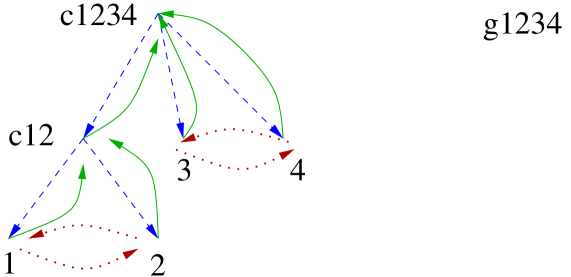
Figure 6: LocateImage is called on the root of the assembly tree $\tau$ shown on the left, for the permutation $g$ shown on right. This permutation $g$ fixes $\tau$. The data structure representing the tree consists of the child (blue, dashed) and parent (green, solid) pointers and the data structure representing $g$ - via its action on the leaf-label set $X$ - consists of $g$-pointers (red, dotted).

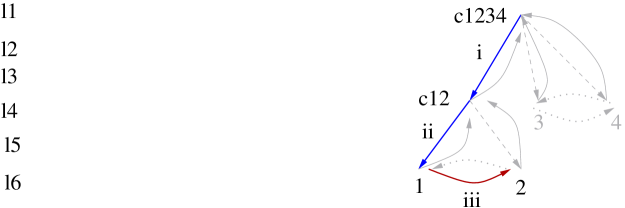
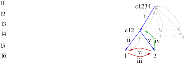
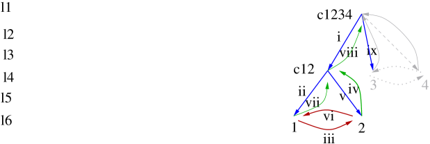
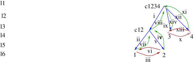
Figure 7: A successful run of LocateImage, where, for all vertices $v$ in $\tau$, the image $g(v)$ is established to be in the assembly-tree $\tau$ shown in Figure 6. On the right are pointers traversed so far, in traversed order. On the left is the current recursion stack of LocateImage calls (first call at the bottom), together with those vertices $v$ ($\in X$ or $\subseteq X$) for which $g(v)$ has been established to be in $\tau$, showing that $g$ is an isomorphism between the two subtrees of $\tau$ rooted at $v$ and at $g(v)$, respectively.

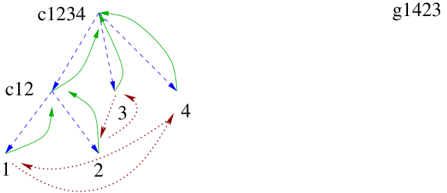
Figure 8: LocateImage is called on the root of the same tree $\tau$ as in Figure 6, but for a different permutation $g$ shown on right. In this case $g$ does not fix $\tau$.

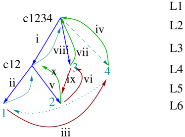
Figure 9: An unsuccessful run of LocateImage. Since $\{1,2\}$, $3$ and $4$ are the children of the root, when LocateImage(root) is called, it checks if their images under $g$ have the same parent. So recursive calls are to LocateImage$(\{1,2\})$, to LocateImage$(3)$, and to LocateImage$(4)$. LocateImage$(\{1,2\})$ returns the root of $\tau$ as a candidate for $g(\{1,2\})$. But LocateImage$(3)$ returns $\{1,2\}$ because the parent of $g(3)=2$ is $\{1,2\}$. Hence LocateImage(root) returns null and Fixes returns ‘false.’

4 Block systems and Fixed Assembly Trees

The formulas in Section 2 for the number of orbits of each size and for the orbit sizes or pathway probabilities (Theorem 3 and Corollary 5) depend on the number of assembly trees fixed by a group. A formula for the number of such fixed trees is the subject of this and the next section.

Recall that an assembly tree $\tau$ is fixed by a group $G$ acting on $X$ if $g(\tau)=\tau$ for all $g\in G$. Two main results of this section (Corollary 11 and Procedure 12) provide a recursive procedure for constructing all trees in ${\mathcal{T}}_{X}$ that are fixed by $G$. This leads, in the next section, to a generating function for the number of such fixed trees. The results in this section depend on a characterization (Theorem 9) of block systems arising from a group acting on a set.

For a group $G$ acting on set $X$, a block is a subset $B\subseteq X$ such that for each $g\in G$, either $g(B)=B$ or $g(B)\cap B=\emptyset$. A block system is a partition of $X$ into blocks. A block system $\bf B$ will be said to be compatible with the group action if $g(B)\in{\bf B}$ for all $g\in G$ and $B\in{\bf B}$. A characterization of complete block systems (Theorem 9) is relevant to the understanding of fixed assembly trees because of the following result. Let $\tau$ be any assembly tree in ${\mathcal{T}}_{X}$. For any vertex $v$ of $\tau$, recall that $v$ is identified with and labeled by its set of descendent leaf-labels. Thus the set of labels of the children of the root is a partition of $X$.

Lemma 8

Let $G$ act on $X$, and let $\tau$ be an assembly tree for $X$ that is fixed by $G$. If $U$ is the set of children of the root of $\tau$, then $U$ is a block system that is compatible with the action of $G$ in $X$.

Proof: For any $v\in U$, let $\tau_{v}$ be the rooted, labeled subtree of $\tau$ that consists of root $v$ and all its descendents. If $\tau$ is fixed by $G$, then $g(\tau)=\tau$ for each $g\in G$. In other words, $g(\tau_{v})=\tau_{u}$ for some $u\in U$. This implies that $g(v)\cap v=\emptyset$ if $u\neq v$ or $g(v)\cap v=v$ if $u=v$. Hence $U$ is block system that is compatible with the action of $G$ on $X$.      

The following notation will be used in this section. The set of orbits of $G$ acting on $X$ will be denoted by ${\bf O}$. For $H\leq G$, let ${\bf C}_{H}$ denote a set of (say left) coset representatives of $H$ in $G$. Note that $|{\bf C}_{H}|=(G:H)$. For $r\in G$ and $Q\subseteq X$, let $r(Q):=\{r(q)\,:\,q\in Q\}$. A group $G$ is said to act simply on $X$ if the stabilizer of each $x$ in $X$ is the trivial group. In this paper, a partition $\Pi$ of a finite set $S$ into $k$ parts is a set $\{\pi_{1},\pi_{2},\cdots,\pi_{k}\}$ of disjoint subsets so that $\cup_{i=1}^{k}\pi_{i}=S$. The subsets $\pi_{i}$ are called the parts of the partition $\Pi$. The order of the parts of a partition is insignificant. That is, $\{\{1,3\},\{2,4\}\}$ and $\{\{2,4\},\{(1,3\}\}$ are identical partitions of the set $\{1,2,3,4\}$. We nevertheless label the parts from $1$ to $k$ for convenience.

Theorem 9

Let us assume that $G$ acts simply on $X$. Let $\Pi=\{\pi_{1},\pi_{2},\dots,\pi_{k}\}$ be a partition of ${\bf O}$ into arbitrarily many parts, and let ${\bf H}=\{H_{1},H_{2},\dots,H_{k}\}$ be a corresponding sets of subgroups of $G$. For each $i$ and each $O\in\pi_{i}$, let $Q_{i,O}$ be any single orbit of the simple action of $H_{i}$ on $O$. Let $Q_{i}=\cup_{O\in\pi_{i}}Q_{i,O}$ and ${\bf Q}=\{Q_{1},Q_{2},\dots,Q_{k}\}$. Let us denote by $(\Pi,{\bf H},{\bf Q})$ the arrangement $\{(\pi_{1},H_{1},Q_{1}),\ldots,(\pi_{k},H_{k},Q_{k})\}$ of each $\pi_{i}$ in $\Pi$ with a corresponding subgroup $H_{i}\leq G$ in ${\bf H}$, and $Q_{i}\in{\bf Q}$.

1. The collection

   $${\bf B}(\Pi,{\bf H},{\bf Q})=\bigcup\limits_{i=1}^{k}\,\bigcup\limits_{r\in{\bf C}_{H_{i}}}r(Q_{i}),$$

   of blocks $r(Q_{i})$ is a compatible block system for $G$ acting on $X$.

2. Every compatible block system for $G$ acting on $X$ is of the above form for some choice of $\Pi,\,{\bf H}$, and $\bf Q$.

3. Two such block systems ${\bf B}(\Pi,{\bf H},{\bf Q})$ and ${\bf B}(\Pi^{\prime},{\bf H}^{\prime},{\bf Q^{\prime}})$ are equal if and only if, there is a permutation $p$ of the set of blocks of $\Pi^{\prime}$ so that for all $i\leq k$, we have $\pi_{p(i^{\prime})}=\pi_{i}$, and for all $i\leq k$, there exists a $g_{i}\in G$ so that $H_{p(i^{\prime})}=g_{i}H_{i}g_{i}^{-1}$, and $Q_{p(i^{\prime})}=g_{i}(Q_{i})$.

Proof: In order to prove Statement (1), let $H\in{\bf H}$ and $B=r(Q)$, where $Q=Q_{i}$ for some $i$. We first show that $B$ is a block. There is a subset $A\subseteq X$ containing at most one element from each $G$-orbit such that $B=rH(A)$. If $g(B)\cap B\neq\emptyset$, then there are elements $a,a^{\prime}\in A$ such that $grh(a)=rh^{\prime}(a^{\prime})$ for some $g\in G$ and $h,h^{\prime}\in H$. Thus $a$ and $a^{\prime}$ are in the same $G$-orbit, which implies that $a=a^{\prime}$. Therefore, $grh(a)=rh^{\prime}(a)$. Since $G$ acts simply, this implies that $grh=rh^{\prime}$, which in turn implies that $gr$ and $r$ are in the same coset of $H$ in $G$. Therefore $g(B)=gr(Q)=r(Q)=B$. This proves, not only that $B$ is a block, but that ${\bf B}(\Pi,{\bf H},{\bf Q})$ is a block system, because ${\bf B}(\Pi,{\bf H},{\bf Q})$ is a partition of $X$ into blocks. Moreover, if $r(Q)\in{\bf B}(\Pi,{\bf H},{\bf Q})$ and $g\in G$, then by definition $gr(Q)\in{\bf B}(\Pi,{\bf H},{\bf Q})$, which shows that ${\bf B}(\Pi,{\bf H},{\bf Q})$ is a block system compatible with $G$.

In order to prove Statement (2), let us denote the set of orbits of $G$ in its action on $X$ by $\{O_{1},O_{2},\dots,O_{n}\}$. We first show that any block $B$ in the action of $G$ on $X$ is of the form $B=B_{1}\cup B_{2}\cup\cdots\cup B_{n}$, where $B_{i}$ is a single orbit of some subgroup $H\leq G$ acting on $O_{i}$. Let $B_{i}=B\cap O_{i}$. Note that $B_{i}=\emptyset$ is a possibility, in which case we have $B=B_{1}\cup B_{2}\cup\cdots\cup B_{m},\,m\leq n$. Each $B_{i}$ itself must be a block because, if $g(B_{i})\cap B_{i}\neq\emptyset$, then $g(B)\cap B\neq\emptyset$. However, $B$ is a block, so $g(B)\cap B\neq\emptyset$ implies that $g(B)=B$, and thus $g(B_{i})=B_{i}$.

Let $H_{i}=\{h\in G\,|\,h(B_{i})=B_{i}\}$. We claim that $H_{1}=H_{2}=\dots=H_{m}$. To see this let $h\in H_{i}$. Since $B$ is a block, either $h(B)\cap B=\emptyset$ or $h(B)=B$. However, $h(B)\cap B=\emptyset$ is impossible because $h(B_{i})=B_{i}$. Hence $h(B)=B$. Now $B_{j}=B\cap O_{j}$ implies, for each $j$, that $h(B_{j})=B_{j}$. Therefore $h_{i}\in H_{j}$ for all $i,j$. This verifies the claim, so let $H=H_{1}=H_{2}=\dots=H_{m}$.

The proof that each block $B$ is of the required form is complete if it can be shown that $H$ acts transitively on $B_{i}$ for each $i$. To see this, let $x,y\in B_{i}$. Since $B_{i}$ lies in a single $G$-orbit, there is a $g\in G$ such that $g(x)=y$. Since $B_{i}$ has been shown to be a block and $g(B_{i})\cap B_{i}\neq\emptyset$, it must be the case that $g(B_{i})=B_{i}$. Therefore $g\in H_{i}=H$.

To complete the proof of Statement (2), let ${\bf B}$ be any compatible block system for $G$ acting on $X$. We have proved that if $B\in{\bf B}$, then $B=B_{1}\cup B_{2}\cup\cdots\cup B_{m}$, where $B_{i}$ is a single orbit of some subgroup $H\leq G$ acting on $O_{i}$. Because of the compatibility, the action of $G$ on $X$ induces an action of $G$ on ${\bf B}$. The orbits under this action provide a partition $\Pi$ of ${\bf O}$, a part $\pi\in\Pi$ consisting of all $G$-orbits acting on $X$ contained in the union of a single $G$-orbit acting on ${\bf B}$. Consider any orbit $W$ of $B$ in this action. If $B^{\prime}$ is another element of $W$, then there is an $r\in G$ such that $B^{\prime}=r(B)$. This shows that the blocks in $G(B)$ are of the desired form in Statement (1) of the theorem. Repeating this argument for each part in the partition $\Pi$ completes the proof of Statement (2).

To prove Statement (3), we first show that if $Q\in{\bf Q}$ is the union of $H$-orbits and $H^{\prime}(Q)=Q$, where $H,H^{\prime}\in{\bf H}$, then $H^{\prime}=H$. Restricting attention to just one orbit of $G$ in its action on $X$, the equality $H^{\prime}(Q)=Q$ implies that $H^{\prime}(a^{\prime})=H(a)$ for some $a,a^{\prime}$ in the same $G$-orbit acting on $X$. Let $g\in G$ be such that $a=g(a^{\prime})$ and hence $Hg(a^{\prime})=H^{\prime}(a^{\prime})$, which in turn implies that $hg(a^{\prime})=a^{\prime}$ for some $h\in H$. Because $G$ acts simply, this implies that $g=h^{-1}\in H$, so $H(a^{\prime})=H^{\prime}(a^{\prime})$, which again, by the simplicity of the action, implies that $H^{\prime}=H$.

Now let us assume that ${\bf B}(\Pi,{\bf H},{\bf Q})={\bf B}(\Pi^{\prime},{\bf H}^{\prime},{\bf Q^{\prime}})$. Clearly, $\Pi=\Pi^{\prime}$. It is sufficient to restrict our attention to just one of the parts in the partition $\Pi=\Pi^{\prime}$, so we must show that $\{r(Q)\,:\,r\in{\bf C}_{H}\}=\{r(Q^{\prime})\,:\,r\in{\bf C}_{H^{\prime}}\}$ if and only if $H^{\prime}=gHg^{-1}$, and $Q^{\prime}=g(Q_{i})$ for some $g\in G$. If $H^{\prime}=gHg^{-1}$, and $Q^{\prime}=g(Q)$ for some $g\in G$, then for any $r\in G$ we have $r(Q^{\prime})=rH^{\prime}(Q^{\prime})=(rgHg^{-1})g(Q)=rgH(Q)$. This shows that $\{r(Q^{\prime})\,:\,r\in{\bf C}_{H^{\prime}}\}\subseteq\{r(Q)\,:\,r\in{\bf C}_{H}\}$, and the opposite inclusion is similarly shown. Conversely, assume that $\{r(Q)\,:\,r\in{\bf C}_{H}\}=\{r(Q^{\prime})\,:\,r\in{\bf C}_{H^{\prime}}\}$. Since $Q^{\prime}\in\{r(Q^{\prime})\,:\,r\in{\bf C}_{H^{\prime}}\}$, we know that $Q^{\prime}=r(Q)$ for some $r\in{\bf C}_{H}\subseteq G$. Now $(rHr^{-1})(Q^{\prime})=(rHr^{-1})(r(Q))=rH(Q)=r(Q)=Q^{\prime}$. By the uniqueness result shown in the preceding paragraph, we get $H^{\prime}=rHr^{-1}$.      

Example 10

Klein 4-group acting on ${\mathcal{T}}_{4}$ (continued).

Continuing the example from the previous section with $G={\mathbb{Z}}_{2}\oplus{\mathbb{Z}}_{2}$ acting simply on $X=\{1,2,3,4\}$, let $K=K_{1}=\{(1)(2)(3)(4),(1\,2)(3\,4)\}$ and $K_{0}$ the trivial subgroup. There are 11 blocks in the action of $K$ on $X$ which are given below:

$$\{1,2,3,4\},\{1,2\},\{3,4\},\{1,3\},\{2,4\},\{1,4\},\{2,3\},\{1\},\{2\},\{3\},\{4\}.$$

The seven block systems for the action of $K$ on $X$ can be found using Theorem 9. In what follows, $\{1,2\}|\{3,4\}$ denotes the orbit $\{1,2\},\{3,4\}$ partitioned into the two parts $\{1,2\}$ and $\{3,4\}$, whereas $\{1,2\},\{3,4\}$ denotes that same orbit partitioned the trivial way, into one part. Note that ${\bf B}\;(\;\{1,2\}|\{3,4\},\;\{K_{0},K\}\;,\;\{2\}|\{3,4\}\;)$, for example, is not included in the list below. This is because, according to Statement (3) in Theorem 9,

$${\bf B}\;(\;\{1,2\}|\{3,4\},\;\{K_{0},K\}\;,\;\{2\}|\{3,4\}\;)=$$

$${\bf B}\;(\;\{1,2\}|\{3,4\},\;\{K_{0},K\}\;,\;\{1\}|\{3,4\}\;).$$

Namely, for $g=(1\,2)(3\,4)$, we have $\{2\}=g(\{1\})$ and $K_{0}=gK_{0}g^{-1}$.

$${\bf B}\;(\;\{1,2\},\{3,4\},\;\{K\},\;\{1,2,3,4\} =\;(1\,2\,3\,4)$$

$${\bf B}\;(\;\{1,2\},\{3,4\},\;\{K_{0}\},\;\{1,3\}\;) =\;(1\,3)(2\,4)$$

$${\bf B}\;(\{1,2\},\{3,4\},\;\{K_{0}\},\;\{1,4\}\;) =\;(1\,4)(2\,3)$$

$${\bf B}\;(\;\{\{1,2\}|\{3,4\},\;\{K,K\},\;\{1,2\},\{3,4\}\;) =\;(1\,2)(3\,4)$$

$${\bf B}\;(\{\{1,2\}|\{3,4\},\;\{K,K_{0}\},\;\{1,2\},\{3\}\;) =\;(1\,2)(3)(4)$$

$${\bf B}\;(\{1,2\}|\{3,4\},\;\{K_{0},K\},\;\{1\},\{3,4\}\;) =\;(1)(2)(3\,4)$$

$${\bf B}\;(\{1,2\}|\{3,4\},\;\{K_{0},K_{0}\},\;\{1\},\{2\}\;) =\;(1)(2)(3)(4)$$

Let $\tau\in{\mathcal{T}}_{X}$ be a tree fixed by $G$ in its action on $T_{X}$. If $U$ denotes the set of children of the root of $\tau$, recall that Lemma 8 states that the set $U$ of labels is a block system. Recall that the label of a vertex is the set of labels of its leaf descendents, and also the label of a vertex is the union of the labels of its children. According to Theorem 9, any block system is of the form

$${\bf B}(\Pi,{\bf H},{\bf Q})=\bigcup\limits_{i=1}^{k}\,\bigcup\limits_{r\in{\bf C}_{H_{i}}}r(Q_{i}).$$

We will use the notation $\tau_{rQ}$ to denote the subtree $\tau_{u},\,u\in U,u=r(Q)$, rooted at $u$. Theorem 9 leads to the characterization of assembly trees fixed by given group $G$ as stated in Corollary 11 below.

Corollary 11

Let us assume that $G$ acts simply on $X$ and that $\tau\in{\mathcal{T}}_{X}$. Let $U$ be the set of children of the root of $\tau$ and, for each $u\in U$, let $\tau_{u}$ be the rooted, labeled subtree of $\tau$ that consists of root $u$ and all its descendents. With notation as in Theorem 9, the tree $\tau$ is fixed by $G$ if and only if, for some $\Pi,\,{\bf H}$ and $\bf Q$, the following two conditions hold.

1. $U={\bf B}(\Pi,{\bf H},{\bf Q})$, hence for each $Q\in{\bf Q}$ and $g\in G$, there is a subtree $\tau_{Q}$ and a subtree $\tau_{gQ}.$

2. $\tau_{gQ}=g(\tau_{Q})$ for every $Q\in{\bf Q}$ and every $g\in G$.

Proof: Let us assume that $\tau$ is fixed by $G$. Condition (1) follows immediately from Lemma 8 and Theorem 9. Concerning Condition (2), for any $g\in G$, the set of leaves of $g(\tau_{Q})$ is $g(Q)$. Hence for $\tau$ to be fixed by $G$ it is necessary that $g(\tau_{Q})=\tau_{gQ}$.

Conversely, let us assume that Conditions (1) and (2) hold. For any $g\in G$ we must show that $g(\tau)=\tau$. By Condition (1), it is sufficient to show that $g$ acting on $\tau$ permutes the set of subtrees in such a manner that $g(\tau_{rQ})=\tau_{grQ}$ for every $H\in{\bf H}$, $\;Q$ the corresponding element of $\bf Q$, and every $r\in{\bf C}_{H}$. However, by Condition (2), $g(\tau_{rQ})=gr(\tau_{Q})=\tau_{grQ}$.      

Theorem 13 below states that the following recursive procedure constructs any assembly tree $\tau\in{\mathcal{T}}_{X}$ fixed by $G$. This will be used to prove Theorem 16 in the next section.

Procedure 12

Recursive construction of any assembly tree fixed by a group $\mathbf{G}$:

1. Partition the set ${\bf O}$ of $G$-orbits of $X$: $\Pi=\{\pi_{1},\pi_{2},\dots,\pi_{k}\}$. Note that the parts of $\Pi$ are labeled $1,2,\cdots,k$ in some arbitrary way.

2. For each $i=1,2,\dots,k$, choose a subgroup $H_{i}\leq G$. (If $\Pi$ has only one part then $H_{i}=G$ is not allowed.)

3. For each $i$, choose a single orbit of $H_{i}$ acting on each of the $G$-orbits in $\pi_{i}$, and let $Q_{i}$ be the union of these $H_{i}$-orbits.

4. Recursively, let $\tau_{Q_{i}}$ be any rooted tree whose leaves are labeled by $Q_{i}$ and which is fixed by $H_{i}$.

5. Let $S_{i}=\{\ r(\tau_{Q_{i}})\ |\ r\in{\bf C}_{H_{i}}\}$ and $S=\cup_{i=1}^{k}\,S_{i}$. Let $\tau$ be the rooted tree whose children are roots of the trees in $S$.

Theorem 13

The set of assembly trees constructed by Procedure 12 is the set of assembly trees fixed by the group $G$.

Proof: In the notation of Theorem 9, Steps (1), (2), and (3) are choosing $(\Pi,{\bf H},{\bf Q})$. Steps (4), (5), and (6) are ensuring that $U={\bf B}(\Pi,{\bf H},{\bf Q})$. Note that the restriction in Step (2) is because otherwise the root of the resulting tree in Step (6) would have only one child. Note also that in Step (5), $S_{i}$ does not depend on the particular set of coset representatives. This follows directly from Step (4).

It is now sufficient to show the following. For any assembly tree $\tau$ satisfying $U={\bf B}(\Pi,{\bf H},{\bf Q})$ for some $(\Pi,{\bf H},{\bf Q})$, Condition (2) in Corollary 11 holds if and only if $\tau$ is constructed by Procedure 12. To show that any assembly tree $\tau$ constructed by Procedure 12 satisfies Condition (2), note that Step (4) implies that, if $Q\in{\bf Q}$ corresponds to $H\in{\bf H}$, then $H(Q)=Q$ and hence $h(\tau_{Q})=\tau_{hQ}=\tau_{Q}$ for all $h\in H$. For $g\in G$, if $g=rh$, where $h\in H$, then $g(\tau_{Q})=rh(\tau_{Q})=r(\tau_{hQ})=r(\tau_{Q})=\tau_{rQ}$, the last equality from Step (5). Again, because $H(Q)=Q$, we have $g(\tau_{Q})=\tau_{rQ}=\tau_{rhQ}=\tau_{gQ}$.

Conversely, if $\tau$ satisfies Condition (2) in Corollary 11, then consider the trees $\tau_{Q_{i}}$ $i=1,2,\dots,k$. These are trees whose leaves are labeled by $Q_{i}$. in Step (4) of Procedure 12. Moreover, by Condition (2) we have $h(\tau_{Q_{i}})=\tau_{hQ_{i}}=\tau_{Q_{i}}$ for all $h\in H_{i}$, so $\tau_{Q_{i}}$ is fixed by $H_{i}$. By Step (5) of Procedure 12 and Condition (2) of Corollary 11 we have $r(\tau_{Q_{i}})=\tau_{rQ_{i}}$ for all $r\in{\bf C}_{H_{i}}$. Therefore the tree $\tau$ is constructed by Procedure 12.      

Remark 14

Enforcing uniqueness in the construction.

The construction in Procedure 12 is not unique, in that it may produce the same fixed assembly tree multiple times depending on the choices in Steps 2 and 3. Condition (3) in Theorem 9 shows that we may enforce uniqueness if we make the following two restrictions.

1. If we choose $(\Pi,{\bf H},{\bf Q})=\{(\pi_{1},H_{1},Q_{1}),\ldots,(\pi_{k},H_{k},Q_{k})\}$ in Steps 1 and 2 of the procedure while constructing a tree $\tau$, and if we also have $(\Pi,{\bf H^{\prime}},{\bf Q^{\prime}})=\{(\pi_{1},H_{1}^{\prime},Q_{1}^{\prime}),\ldots,(\pi_{k},H_{k}^{\prime},Q_{k}^{\prime})\}$ during the construction of another tree $\tau^{\prime}$, then to ensure that $\tau\neq\tau^{\prime}$ we need to ensure that for at least one $i$, the group $H_{i}^{\prime}$ should not be conjugate to $H_{i}$ in $G$.

2. Consider the construction of two trees $\tau$ and $\tau^{\prime}$ with corresponding $(\Pi,{\bf H},{\bf Q})$ and $(\Pi,{\bf H^{\prime}},{\bf Q^{\prime}})$ such that for each $i$, the subgroup $H_{i}$ is a conjugate of the subgroup $H_{i}^{\prime}$. Further assume that in Step (3) for the tree $\tau$ the element $g_{i}\in H_{i}$ is such that $g_{i}H_{i}g_{i}^{-1}=H_{i}^{\prime}$. Then while constructing tree $\tau^{\prime}$, we need to ensure that there is at least one $i$ such that $Q_{i}^{\prime}\neq g_{i}(Q_{i})$. (Note that for a given index $i$, there may well be several elements $g_{i}\in G$ so that $g_{i}H_{i}g_{i}^{-1}=H_{i}^{\prime}$ holds, and all those are subject to this restriction.)

Example 15

Klein 4-group acting on ${\mathcal{T}}_{4}$ (continued).

With $G={\mathbb{Z}}_{2}\oplus{\mathbb{Z}}_{2}$ acting on $X=\{1,2,3,4\}$, consider the assembly trees $\tau$ fixed by the subgroup $K=\{(1)(2)(3)(4),(1\,2)(3\,4)\}$. There are exactly six such trees, those in the orbits $A,B,C,D,E$ of Figure 5. These correspond (not in corresponding order) to the block systems in Example 10. Because of the restriction in Step (2) of Procedure 12, the first block system in the list in Example 10 is ignored.

4.1 When the action of $G$ on $X$ is not simple

Let us assume that $G$ acts on $X$, but not necessarily simply. For $q\in X$, let $S_{q}$ denote the stabilizer of $q$ in $G$. For a subset $Q\subseteq X$, let

$$S_{Q}=\bigcup_{q\in Q}S_{q}.$$

If $G$ acts simply on $X$, then the stabilizer of any $x\in X$ is the trivial subgroup. Therefore, in this case, it is clear that $S_{Q}\subset H$ for any $Q\subseteq X$ and $H\leq G$. In the general case, when $G$ acts not necessarily simply on $X$, let us call a pair $(H,Q)$ viable if

$${\bf S}_{Q}\subseteq H.$$

If only viable pairs $(H_{i},Q_{i})$ are allowed in the hypothesis of Theorem 9, then the theorem is valid in the general, not necessarily simple, case. Since this general version of Theorem 9 and associated analogs of Procedure 12 and Theorem 13 are not needed in subsequent sections, and the proofs are relatively straightforward extensions, we omit them.

5 Enumerating Fixed Assembly Trees

Let us assume in this section that $G$ acts simply on each of an infinite sequence $X_{1},X_{2},\dots$ of sets where, by formula (1) we have $|X_{n}|=n|G|$. In other words, $n$ is the number of orbits of $G$ in its action on $X_{n}$. Denote by $t_{n}(G)$ the number of trees in ${\mathcal{T}}_{n}:={\mathcal{T}}_{X_{n}}$ that are fixed by $G$. In this section we provide a formula for the exponential generating function

$$f_{G}(x):=\sum_{n\geq 1}t_{n}(G)\,\frac{x^{n}}{n!}$$

for the sequence $\{t_{n}(G)\}$. If $G$ is the trivial group of order one, then let us denote this generating function simply by $f(x)$. This is the generating function for the total number of rooted, labeled trees with $n$ leaves in which every non-leaf vertex has at least two children. For $H\leq G$, let

$$\widehat{f}_{H}(x)=\frac{1}{(G:H)}\;f_{H}\left((G:H)x\right).$$

Theorem 16

The generating function $f_{G}(x)$ satisfies the following functional equations:

$$1-x+2f(x)=\exp\,(f(x)),$$

and for $|G|>1$,

$$1+2f_{G}(x)=\exp\,\left(\sum_{H\leq G}\;\widehat{f}_{H}(x)\right).$$

Proof: The first formula is proved in [20], page 13. For $|G|>1$, we use the standard exponential and the product formulas for generating functions.

The proof of the second formula uses two well known results from the theory of exponential generating functions, the “product formula” and the “exponential formula”. In Procedure 12, give Steps (3) and (4) the name putting an $H_{i}$-structure on $\pi_{i}$. According to Theorem 13, the number of trees $t_{n}(G)$ fixed by $G$ equals the number of ways to partition the set of orbits of $G$ acting on $X_{n}$ and to place an $H$-structure on each part in the partition, for some subgroup $H\leq G$, keeping the uniqueness Remark 14 in mind.

In Step (3) of Procedure 12, since $G$ acts simply and the number of $H_{i}$-orbits in one $G$-orbit is $|G|/|H_{i}|=(G:H_{i})$, the number of possible choices for $Q_{i}$ (the union of these single $H_{i}$-orbits) is $(G:H)^{m}$. Hence, in accordance with Step (4) of Procedure 12, the generating function for the number of ways to place an $H$-structure is basically $f_{H}((G:H)x)$.

However, this must be altered in accordance with the uniqueness requirements in Remark 14. Let ${\bf N}$ denote a set consisting of one representative of each conjugacy class in the set of subgroups of $G$. By Statement (a) in Remark 14, only subgroups in ${\bf N}$ are considered. Let $N(H):=\{g\in G\,|\,gHg^{-1}=H\}$ denote the normalizer of $H$ in $G$. By Statement (b), there has to be an index $i$ so that $g(Q_{i})\neq Q_{i}^{\prime}$. However, $g(Q_{i})=g^{\prime}(Q_{i})$ will occur for every $i$ if and only if $g$ and $g^{\prime}$ are in the same coset of $H$ in $G$. Therefore, the generating function for the number of ways to place an $H$-structure is $\frac{1}{(N(H):H)}\;f_{H}((G:H)x)$.

The exponential formula states that the generating function $g_{H}(x)=\sum_{n\geq 0}a_{n}\,\frac{x^{n}}{n!}$ for the number of ways $a_{n}$ to partition the set of $G$-orbits acting on $X_{n}$ and, on each part $\pi$ in the partition, place an $H$-structure (same $H$) is

$$g_{H}(x):=\exp\left(\widehat{f}_{H}(x)\right).$$

Here we assume that $a_{0}=1$.

The generating function for the number of ways to partition the set of orbits, i.e., choose $\Pi=(\pi_{1},\pi_{2},\dots,\pi_{k})$ and, on each part of the partition, place an $H$-structure, one $H$ from each conjugacy class in ${\bf N}$ is

$$\prod_{H\in{\bf N}}g_{H}(x) =\prod_{H\in{\bf N}}\exp\left(\frac{1}{(N(H):H)}\;f_{H}((G:H)x)\right)$$

$$=\exp\,\left(\sum_{H\in{\bf N}}\;\frac{1}{(N(H):H)}\;f_{H}((G:H)x)\right).$$

Note that we have not taken the restriction in Step (2) of Procedure 12 into consideration. Taking the partition of the orbit set into just one part and placing on that part a $G$-structure results in counting the number of fixed trees a second time. Also since the constant term in $\prod_{H\in{\bf N}}g_{H}(x)$ is 1,

$$1+2\,f_{G}(x) =\exp\,\left(\sum_{H\in{\bf N}}\;\frac{1}{(N(H):H)}\;f_{H}((G:H)x)\right)$$

$$=\exp\,\left(\sum_{H\leq G}\;\frac{1}{(G:H)}\;f_{H}((G:H)x)\right).$$

Here the last equality holds because $f_{H}(x)$ depends only the conjugacy class of $H$ in $G$ and

$$\frac{1}{(N(H):H)}\Big{/}\frac{1}{(G:H)}=\frac{(G:H)}{(N(H):H)}=(G:N(H))=|{\bf N}|.$$

     

Example 17

Klein 4-group acting on ${\mathcal{T}}_{4}$ (continued).

Consider $G={\mathbb{Z}}_{2}\oplus{\mathbb{Z}}_{2}$ acting on $X_{n}$. Recall that $X_{n}=4n$, the integer $n$ being the number of $G$-orbits. In this case ${\bf N}=\{K_{0},K_{1},K_{2},K_{3},G\}$, where $K_{0}$ is the trivial group and

$$K_{1} =\{\,(1)(2)(3)(4),(1\;2)(3\;4)\,\},$$

$$K_{2} =\{\,(1)(2)(3)(4),(1\;3)(2\;4)\,\},$$

$$K_{3} =\{\,(1)(2)(3)(4),(1\;4)(2\;3)\,\}.$$

The functional equations in the Statement of Theorem 16 are

$$1-x+2f(x) =\,\exp\,(f(x))$$

$$1+2f_{K_{i}}(x) =\,\exp\,\left(\frac{1}{2}\,f(2x)+f_{K_{i}}(x)\right)\quad\text{for $i=1,2,3$, and}$$

$$1+2f_{G}(x) =\,\exp\,\left(\frac{1}{4}\,f(4x)+\frac{1}{2}\,f_{K_{1}}(2x)+\frac{1}{2}\,f_{K_{2}}(2x)+\frac{1}{2}\,f_{K_{3}}(2x)+f_{G}(x)\right).$$

Using these equations and MAPLE software, the coefficients of the respective generating functions provide the following first few values for the number of fixed assembly trees. For the first entry $t_{1}(G)=4$ for the group $G$, the four fixed trees are shown in Figure 5 $A$, $B$, $C$, $D$. For trees with eight leaves there are $t_{2}(G)=104$ assembly trees fixed by $G={\mathbb{Z}}_{2}\oplus{\mathbb{Z}}_{2}$, and so on.

$$t_{n}(K_{0}) :\quad 1,1,4,26,236,2752$$

$$t_{n}(K_{i}) :\quad 1,6,72,1312,32128,989696$$

$$t_{n}(G) :\quad 4,104,4896,341120,31945728,3790876672.$$

Theorem 16 provides the generating function for the numbers $t_{n}(H)$ of fixed assembly trees in the action of any subgroup $H\leq G$ on $X_{n}$. What is required for Problem (i) described in Sections 1 and 2 are the numbers $\overline{t}_{n}(H)$ of assembly trees that are fixed by $H$, but by no other elements of $G$. In Example 15, for $G={\mathbb{Z}}_{2}\oplus Z_{2}$ acting on $X=\{1,2,3,4\}$, there are six trees that are fixed by the subgroup $K=\{\,(1)(2)(3)(4),(1\;2)(3\;4)\,\}$. However, of these six, four ($A$, $B$, $C$, and $D$ in Figure 5) are also fixed by $G$. Therefore there are only two assembly trees fixed by $K$ and no other elements of $G$ (these are $E$, and $F$ in Figure 5). In general, as shown Theorem 2, Möbius inversion [22] can be used to calculate the values of $\overline{t}_{X}(H)$ from the values of $t_{X}(H)$.

6 The Icosahedral Group

For completeness, the results of the previous sections are applied to the motivating $T=1$ viral example. An isometry of 3-space is a bijective transformation that preserves length, and an isometry is called direct if it is orientation preserving. Rotations, for example, are direct, while reflections are not. A symmetry of a polyhedron is an isometry that keeps the polyhedron, as a whole, fixed, and a direct symmetry is similarly defined. The icosahedral group is the group of direct symmetries of the icosahedron. It is a group of order 60 denoted $G_{60}$.

As mentioned earlier, the viral capsid is modeled by a polyhedron $P$ with icosahedral symmetry, whose set $X$ of facets represent the protein monomers. The icosahedral group, acts on $P$ and hence on the set $X$. It follows from the quasi-equivalence theory of the capsid structure that $G_{60}$ acts simply on $X$. Formula (1) shows that $|X|:=|X_{n}|=60n$, where $n$ is the number of orbits. Not every $n$ is possible for a viral capsid; $n$ must be a $T$-number as defined in the introduction. Before the number of orbits of each size for the action of $G_{60}$ on the set ${\mathcal{T}}_{n}:={\mathcal{T}}_{X_{n}}$ of assembly trees can be determined, basic information about the icosahedral group is needed.

The group $G_{60}$ consists of:

• the identity,

• 15 rotations of order 2 about axes that pass through the midpoints of pairs of diametrically opposite edges of $P$,

• 20 rotations of order 3 about axes that pass through the centers of diametrically opposite triangular faces, and

• 24 rotations of order 5 about axes that pass through diametrically opposite vertices.

There are 59 subgroups of $G_{60}$ that play a crucial role in the theory. Besides the two trivial subgroups, they are the following:

• 15 subgroups of order 2, each generated by one of the rotations of order 2,

• 10 subgroups of order 3, each generated by one of the rotations of order 3,

• 5 subgroups of order 4, each generated by rotations of order 2 about perpendicular axes,

• 6 subgroups of order 5, each generated by one of the rotations of order 5,

• 10 subgroups of order 6, each generated by a rotation of order 3 about an axis L and a rotation of order 2 that reverses L,

• 6 subgroups of order 10, each generated by a rotation of order 5 about an axis L and a rotation of order 2 that reverses L,

• 5 subgroups of order 12, each the symmetry group of a regular tetrahedron inscribed in $P$.

From the above geometric description of the subgroups, it follows that all subgroups of a given order are conjugate in the group $G_{60}$. Representatives of the conjugacy classes of the subgroups of the icosahedral group are denoted by $G_{0},G_{2},G_{3},G_{5},G_{6},G_{10},G_{12},G_{60}$, where the subscript is the order of the group. The set of subgroups of $G_{60}$ forms a lattice, ordered by inclusion. A partial Hasse diagram for this lattice $\bf L$ is shown in Figure 10. The number on the edge joining $G_{i}$ (below) and $G_{j}$ (above) indicate the number of distinct subgroups of order $i$ contained in each subgroup of order $j$. The number in parentheses on the edge joining $G_{i}$ (below) and $G_{j}$ (above) indicate the number of distinct subgroups of order $j$ containing each subgroup of order $i$. It is well-known that any finite partially ordered set $P$ admits a Möbius function $\mu\,:\,P\times P\rightarrow\mathbb{Z}$. The Möbius function of $\bf L$ is shown in Table 1. The entry in the table corresponding to the row labeled $G_{i}$ and column $G_{j}$ is $\mu(G_{i},G_{j})$.

Figure 10: Partial Hasse diagram for the lattice of subgroups of the icosahedral group.

Table 1: The values of the Möbius function of the subgroup lattice of $G_{60}$.

For $|X|=60$, i.e., for the $T=1$ polyhedral case, using Theorem 16 and MAPLE software, the generating functions $f_{G_{i}}(x)$ were computed, and hence their coefficients $t_{60/i}(G_{i})$ which count the number of assembly trees that are fixed by $G_{i}$ were also be computed. Note that since $|X|=60$, the number of orbits of $G_{i}$ in its action on $X$ is $60/i$. Substituting these values into Theorem 2 and using the Möbius Table 1 yields the following numerical values for $\overline{t}_{i}(G_{60/i})$, the number of assembly trees over $X$ with $|X|=60$ that are fixed by $G_{i}$ but by no other elements of $G_{60}$. In other words, these are the numbers of trees whose stabilizer in $G_{60}$ is $G_{i}$.

$${\overline{t}}_{60}(G_{1}) =1924465510132437394720184730922187571120346754532$$

$$\quad 2366329965115755432139023628289410324670840066578537680$$

$${\overline{t}}_{30}(G_{2}) =1670856367100496379411587456529324583988755126499875584$$

$${\overline{t}}_{20}(G_{3}) =10087157294451731428720995944759704$$

$${\overline{t}}_{15}(G_{4}) =10041342673530270014535171213312$$

$${\overline{t}}_{12}(G_{5}) =20540071766413107840$$

$${\overline{t}}_{10}(G_{6}) =61346927354448105268$$

$${\overline{t}}_{6}(G_{10}) =223503950260$$

$${\overline{t}}_{5}(G_{12}) =16865654580$$

$${\overline{t}}_{1}(G_{60}) =204$$

From Theorem 3, the above numbers $\overline{t}_{i}(G_{60/i})$ tell us the number of assembly trees with orbit size $i$, or in other words, trees in an assembly pathway of size $i$. That is, the probability of such a pathway is $i/|\mathcal{T}_{X}|$.

It is worth comparing the first and last elements of this list. While the individual pathways belonging to $G_{1}$ are only 60 times more probable then those that belong to $G_{60}$, there are about $10^{99}$ times more of them.

7 Conclusion and Open Problems

We have developed an algorithmic and combinatorial approach to a problem arising in the modeling of viral assembly. Our results illustrate, not only that problems arising from structural biology can be of independent mathematical interest, but also that mathematical methods have a direct application in structural biology.

More specifically, we have developed techniques to analyze the probability of a capsid forming along a given assembly pathway. One remaining issue is how to extend these techniques to finding the probability of valid assembly pathways as defined in Section 1. As mentioned earlier, valid assembly trees can be defined combinatorially, using generalized notions of connectivity of the polyhedral graph whose facets form the leaves of the tree. Combining such graph theoretic restrictions with our techniques will likely require new ingredients. A second important issue is how to extend our techniques to nucleation in viral shell assembly. Mathematically [3], the problem is to estimate the proportion of valid assembly trees that have a subtree whose leaves form a specific subset of facets, for example a trimer or a pentamer, in the underlying polyhedron.

In addition to the above extensions of the theory, there is scope to tighten some results of the paper. For example, a finer complexity analysis for Algorithm Stabilizer could be based on using Sim’s algorithm, strong generating sets, and the Cayley graph for $G$ as input.

A study of unlabeled trees that are $g$-unfixable may lead to relevant related results. Let us say that a tree is $g$-unfixable if there is no leaf-labeling so that the resulting labeled tree is fixed by the permutation $g$, and let us say that a tree is $G$-unfixable if it is $g$-unfixable for every nontrivial element of the group $G$. These properties are interesting for at least two reasons. First, they clarify the minimum quantifiable information in a labeled tree that is needed for deciding if it is fixed by a group element $g$: if the underlying unlabeled tree is $g$-unfixable, then the information in the labeling is unnecessary to make this decision. This may lead to efficient algorithms and tight complexity bounds. Second, in the language of formal logic, these properties are likely to be monadic second order expressible [7, 24], permitting the application of limit laws for the asymptotic probabilities of finite structures satisfying such properties.

References

- [1] M. Agbandje-McKenna, A.L. Llamas-Saiz, F. Wang, P. Tattersall and MG Rossmann. Functional implications of the structure of the murine parvovirus, minute virus of mice. Structure, 6:1369–1381, 1998.
- [2] B. Berger and P.W. Shor. Local rules switching mechanism for viral shell geometry, Technical report, MIT-LCS-TM-527, 1995.
- [3] M. Bóna and M. Sitharam Influence of symmetry on probabilities of icosahedral viral assembly pathways, Computational and Mathematical Methods in Medicine: Special issue on Mathematical Virology, Stockley and Twarock Eds, 2008.
- [4] B. Berger, P. Shor, J. King, D. Muir, R. Schwartz and L. Tucker-Kellogg. Local rule-based theory of virus shell assembly, Proc. Natl. Acad. Sci. USA, 91:7732–7736, 1994.
- [5] Gunnar Brinkmann and Andreas Dress. A constructive enumeration of fullerenes, Journal of Algorithms., 23:345–358, 1997.
- [6] D. Caspar and A. Klug. Physical principles in the construction of regular viruses, Cold Spring Harbor Symp Quant Biol, 27:1–24, 1962.
- [7] K.J. Compton. A logical approach to asymptotic combinatorics II: monadic second-order properties, J. Comb. Theory Ser. A 50(1):110–131, 1989.
- [8] W.H.E. Day. Optimal algorithms for comparing trees with labeled leaves, Journal of Classification, 2(1):7–26, 1985.
- [9] M. Deza and M. Dutour. Zigzag structures of simple two-faced polyhedra, Combin. Probab. Comput., 14(1-2):31–57, 2005.
- [10] M. Deza, M. Dutour, and P. W. Fowler. Zigzags, railroads, and knots in fullerenes, Chem. Inf. Comp. Sci., 44:1282–1293, 2004.
- [11] P. Gawron, V. V. Nekrashevich, and V. I. Sushchanskii, Conjugacy classes of the automorphism group of a tree Mathematical Notes 65(6):787-790, 1999.
- [12] J. E. Johnson and J. A. Speir. Quasi-equivalent viruses: a paradigm for protein assemblies, J. Mol. Biol., 269:665–675, 1997.
- [13] M.H. Klin. On the number of graphs for which a given permutation group is the automorphism group (Russian), English translation: Kibernetika 5:892-870, 1973.
- [14] C. J. Marzec and L. A. Day. Pattern formation in icosahedral virus capsids: the papova viruses and nudaurelia capensis virus, Biophys, 65:2559–2577, 1993.
- [15] D. Rapaport, J. Johnson and J. Skolnick. Supramolecular self-assembly: molecular dynamics modeling of polyhedral shell formation, Comp Physics Comm, 1998.
- [16] V. S .Reddy, H. A. Giesing, R. T. Morton, A. Kumar, C.B. Post, C. L. Brooks, and J. E. Johnson. Energetics of quasiequivalence: computational analysis of protein-protein interactions in icosahedral viruses. Biophys, 74:546–558, 1998.
- [17] Á. Seress. Permutation Group Algorithms, Cambridge University Press, 2003.
- [18] M. Sitharam and M. Agbandje-McKenna. Modeling virus assembly using geometric constraints and tensegrity:avoiding dynamics, Journal of Computational Biology, 13(6):1232–1265, 2006.
- [19] M. Sitharam and M. Bóna. Combinatorial enumeration of macromolecular assembly pathways, In Proceedings of the International Conferecnce on bioinformatics and applications. World Scientific, 2004.
- [20] R. Stanley. Enumerative Combinatorics, Volume 2, Cambridge University Press, 1999.
- [21] G. Valiente. Algorithms on Trees and Graphs, Springer, 2002.
- [22] J.H. van Lint and R.M. Wilson. A Course in Combinatorics, Cambridge University Press, 2006.
- [23] S. G. Wagner. On an identity for the cycle indices of rooted tree automorphism groups Electronic Journal of Combinatorics, 13:450–456, 2006.
- [24] A. R. Woods, Coloring rules for finite trees and probabilities of monadic second order sentences, Random Structures and Algorithms, 10(4):453–485, 1998.
- [25] A. Zlotnick, R Aldrich, J. M. Johnson, P. Ceres, and M. J. Young. Mechanisms of capsid assembly for an icosahedral plant virus, Virology, 277:450–456, 2000.
- [26] A Zlotnick. To build a virus capsid: an equilibrium model of the self assembly of polyhedral protein complexes. J. Mol. Biol., 241:59–67, 1994.
- [27] A. Zlotnick, J. M. Johnson, P.W. Wingfield, S.J. Stahl, and D. Endres. A theoretical model successfully identifies features of hepatitis b virus capsid assembly, Biochemistry, 38:14644–14652, 1999.