Soliton strings and interactions in mode-locked lasers

Abstract

Soliton strings in mode-locked lasers are obtained using a variant of the nonlinear Schrödinger equation, appropriately modified to model power (intensity) and energy saturation. This equation goes beyond the well-known master equation often used to model these systems. It admits mode-locking and soliton strings in both the constant dispersion and dispersion-managed systems in the (net) anomalous and normal regimes; the master equation is contained as a limiting case. Analysis of soliton interactions show that soliton strings can form when pulses are a certain distance apart relative to their width. Anti-symmtetric bi-soltion states are also obtained. Initial states mode-lock to these states under evolution. In the anomalous regime individual soliton pulses are well approximated by the solutions of the unperturbed nonlinear Schrödinger equation, while in the normal regime the pulses are much wider and strongly chirped.

1 Introduction

Ultra-short pulses in mode-locked (ML) lasers are the topic of extensive research due to their wide range of applications ranging from communications [1], to optical clock technology [2] and even to measurements of the fundamental constants of nature [3]. Although ML lasers have been studied for many years [4, 1] it is only recently that researchers have begun to fully understand and explore their complicated dynamics. Here we discuss pulses associated with a model equation which has both power (intensity) and energy saturation. This equation goes beyond the well-known master equation [5, 1] which is contained in the limiting case of small power. The master equation has gain and filtering terms which are saturated by energy; there is an additional nonlinear gain/loss term which grows with power (intensity). On the other hand, this model critically differs by having the loss term saturated by power (intensity). We show below that this equation admits soliton strings, including anti-symmetric bi-soliton states, in both the anomalous and normal regimes and these modes can mode-lock from initial states under evolution, i.e. we find these soliton states to be attractors. These results are consistent with observations from recent experiments in both the anomalous [6, 7] and normal [8] regimes where in the latter case higher-order anti-symmetric solitons (or bi-solitons) were observed.

A simplified equation without gain/loss terms which is sometimes used to model ultrashort pulses in mode-locked (ML) lasers is the “classical” nonlinear Schrödinger (NLS) equation. The NLS equation in the anomalous regime exhibits both fundamental and high-order soliton solutions. While the fundamental solutions (single solitons) are stationary the higher states exhibit nontrivial evolution. In the normal regime the NLS equation does not have localized decaying solutions. Indeed, the NLS equation has only dark solitons, namely states that do not decay at infinity but form on a nontrivial background. On the other hand to properly describe ML lasers, in addition to chromatic dispersion and Kerr nonlinearity (self-phase modulation), saturable gain, filtering and intensity discrimination should be taken into account. In this regard, the so-called master equation [5, 1] is an important extension of the NLS equation modified accordingly to contain gain and filtering saturated by energy (the time integral of the pulse power), while there is an additional (sign dependent) cubic nonlinear term that takes into account additional gain/loss. The master equation has only a small parameter regime where mode-locking to stable soliton states occurs [9]; it has not been shown to support higher-order states. In fact, for certain values of the parameters this equation exhibits a range of phenomena including: mode-locking evolution, pulses which disperse into radiation, and some whose amplitude grows rapidly [10]. In the latter case, if the nonlinear gain is too high, the linear attenuation terms are unable to prevent the pulse from blowing up, suggesting the breakdown of the master mode-locking model [9]. Thus an improved model is desirable.

If the pulse energy is taken to be constant the master equation reduces to a cubic nonlinear Ginzburg-Landau (GL) type system. Such GL systems in the anomalous regime have been found to support steady high-order soliton solutions [11]; they also contain a wide range of solutions including unstable, chaotic and quasi-periodic states and even blow-up can occur. Furthermore, soliton interaction within the framework of such GL systems is complicated. It is found [11] that both in-phase and anti-phase high-order soliton states are either unstable or weakly stable. In either case these states are not attractors [12]. Hence they do not correspond to observations of higher order soliton states in a ML laser system which has discrete, nearly fixed separations [6]. Furthermore, these GL equations do not exhibit stable pulses in the normal regime [7].

The distributive both power (intensity) and energy saturation model which we refer to as the power-energy saturation (PES) equation is given in nondimensional form as

$$i\psi_{z}+\frac{d(z)}{2}\psi_{tt}+n(z)|\psi|^{2}\psi=$$

$$\frac{ig}{1+\epsilon E}\psi+\frac{i\tau}{1+\epsilon E}\psi_{tt}-\frac{il}{1+\delta P}\psi$$ (1)

where $\psi(z,t)$ is the slowly varying electromagnetic pulse envelope, $E(z)=\int_{-\infty}^{+\infty}|\psi|^{2}dt$ is the pulse energy, $P(z,t)=|\psi|^{2}$ is the instantaneous pulse power and the parameters $g$, $\tau$, $l$, $\epsilon$, $\delta$ are all positive, real constants. The dispersion is represented by $d(z)$, which is taken to either be constant ($d(z)=d_{0}>0$ corresponds to the anomalous regime while $d(z)=d_{0}<0$ represents normal) or a dispersion-managed system (see Section 5). The dimensionless nonlinear coefficient will be taken to be unity ($n(z)=1$) in the first part of the article and varying between zero and one in the dispersion-managed case, as holds in many experiments [13, 14]. The first term on the right hand side represents gain-saturated by energy, the second is spectral filtering-saturated by energy and the third is loss saturated by power (intensity). The coefficients $\epsilon$, $\delta$ are related to the saturation energy and power respectively. If we expand the denominator of the loss term in a Taylor series in the limit of small power and keep only the first two terms, we reduce to the master-equation! Furthermore, if one expands the power saturation term in Eq. (1) and keep higher order nonlinearities (e.g. fifth order nonlinearities) higher nonlinear GL systems result. The energy and power saturation terms in Eq. (1) are essentially the simplest such forms (inversely linear in their saturation effects). This type of power saturated loss has been used in lumped models to describe experimental ML pulses [13, 8] and is widely used as a saturable loss model (e.g. semiconductor saturable loss mirrors–SeSAMs). In [15, 16] the distributive model was employed to show that single soliton states model-lock over a large region of parameter space. More recently it was shown [17] that dispersion-managed models with power (intensity)-energy saturation are in good agreement with experimental results in mode-locked Ti:sapphire lasers. It is therefore important to study the above distributed model.

Dimensional values associated with a typical Ti:Sapphire laser system are [18]: $\beta^{\prime\prime}=60\mathrm{fs}^{2}/\mathrm{mm}$ is the group velocity dispersion, $\gamma=1\mathrm{/cmMW}$ the nonlinear coefficient $P_{*}=5\mathrm{MW}$ the characteristic power, $E_{*}=P_{*}t_{*}$ the characteristic energy, $z_{*}=2\mathrm{mm}$ the corresponding characteristic-nonlinear length ($z_{*}=1/\gamma P_{*}$), $t_{*}=10\mathrm{fs}$ the characteristic time, $g_{*}=20\mathrm{dB}$ the dimensional gain, $l_{*}=0.15\mathrm{1/mm}$ the dimensional distributive saturable loss parameter, $\Delta\omega=100$ THZ the frequency cutoff, $E_{\mathrm{sat}}=10\mathrm{nJ}$ and $P_{\mathrm{sat}}=2\mathrm{MW}$ are the saturated energy and power, respectively. Hence: $d_{0}=\beta^{\prime\prime}z_{*}/t_{*}^{2}$, $g=g_{*}z_{*}$, $\tau=g_{*}z_{*}/\Delta\omega^{2}t_{*}^{2}$, $\epsilon=E_{*}/E_{\mathrm{sat}}$ and $\delta=P_{*}/P_{\mathrm{sat}}$. These dimensional values lead to phenomena which are consistent with the results presented in this article.

2 Constant dispersion systems

The effects of energy and power saturation are crucial in both the anomalous and normal regimes. From ML laser behavior, the gain and filtering mechanisms are related to the energy of the pulse, while the loss is related to the power (intensity) of the pulse. Indeed, passive mode-locking generally utilizes saturable absorbers which are modeled here by a distributive loss term saturated with power.

In the constant anomalous regime $(d(z)=d_{0}>0)$ the saturation terms help localize an intense pulse preventing it from reaching a singular state; i.e. “infinite” energy or a blow-up in amplitude does not result. Indeed, if blow-up were to occur that would mean that both the amplitude and the energy of the pulse are large, hence, the perturbing effects are very small thus reducing Eq. (1) to the unperturbed NLS equation, which admits a stable, finite solution. In addition, when localization occurs, the perturbing effects are small essentially reducing the equation to the unperturbed NLS equation. Indeed, it has been shown [16] that when mode-locking occurs the resulting individual pulses are essentially solitons of the unperturbed NLS equation; the perturbing influence of these terms yields the mode-locking mechanism.

In the constant normal regime $(d(z)=d_{0}<0)$, three regimes are observed [19]: (a) when the loss is much greater than the gain the pulse decays to zero, (b) when the loss is again the prominent effect but sufficient gain exists in the system to sustain a very slowly decaying evolution resulting in a “quasi-soliton” state and (c) the soliton regime above a certain value of gain. This soliton differs from its anomalous dispersion counterpart in that it does not obey the unperturbed NLS equation, it is much wider and strongly chirped.

For example in Fig. 1 a soliton mode is depicted which evolves from a unit gaussian state in the anomalous ($d_{0}=1$) and normal ($d_{0}=-1$) regimes (here $\tau=l=0.1$, $\epsilon=\delta=1$ and $g=0.5$ in the anomalous case, $g=1.5$ in the normal case)

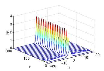
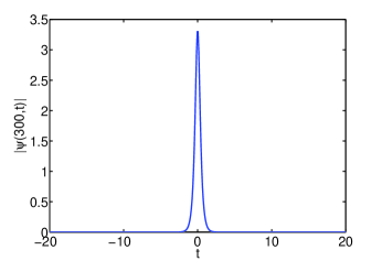
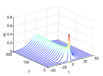
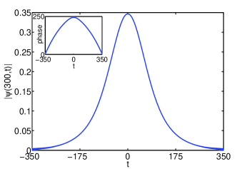
Figure 1: (Color online) Mode-locking evolution for a single soliton evolving from a unit gaussian initial state in the anomalous (top two figures) and normal (bottom two figures) regimes; states at $z=300$ are depicted below each evolution. For the normal regime the phase-chirp is shown in the inset.

High-order solitons of the anomalous regime $(d_{0}=1>0)$ are discussed first. Here solitons are obtained when the gain is above a certain critical value, $g>l$, otherwise pulses dissipate and eventually vanish [16]. As gain becomes stronger additional soliton states are possible and 2, 3, 4 or more coupled pulses are found to be supported. Here we set $\tau=l=0.1$, $\epsilon=\delta=1$ and vary the gain parameter $g$. The value of $\Delta\xi/\alpha$, where $\Delta\xi$ and $\alpha$ are the pulse separation and pulse width respectively, is an important parameter. The full width of half maximum (FWHM) for pulse width is used, $\Delta\xi,$ is measured between peak values of two neighboring pulses and $\Delta\phi$ is the phase difference between the peak amplitudes. With sufficient gain $(g=0.5)$ Eq. (1) is evolved starting from unit gaussians with initial peak separation $\Delta\xi=10$ and $\Delta\xi/\alpha=8.5$. The evolution and final state are depicted in Fig. 2.

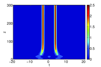
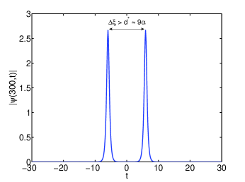
Figure 2: (Color online) Mode-locking evolution for an in phase two soliton state of the anomalously dispersive PES (top) equation and the resulting soliton profile (bottom) at $z=300$. Here $g=0.5$.

For the final state we find $\Delta\xi/\alpha\approx 10$. The resulting individual pulses are similar to the single soliton mode-locking case [16], i.e. individual pulses are approximately solutions of the unperturbed NLS equation, namely hyperbolic secants. The pulses differ from a single soliton in that the individual pulse energy is smaller then that observed for the single soliton mode-locking case for the same choice of $g$, while the total energy of the two soliton state is higher. This is due to the non-locality of energy saturation in the gain and filtering terms.

To investigate the minimum distance, $d^{*}$, between the solitons in order for no interactions to occur we evolve equation starting with two solitons. If the initial two pulses are sufficiently far apart then the propagation evolves to a two soliton state and the resulting pulses have a constant phase difference. If the distance between them is less than a critical value then the two pulses interact in a way characterized by the difference in phase between the peaks amplitudes: $\Delta\phi$. When initial conditions are symmetric (in phase) two pulses are found to merge into a single soliton of Eq. (1). When the initial conditions are anti-symmetric (out of phase by $\pi$) then they repel each other until their separation is above this critical distance while retaining the difference in phase, resulting in an effective two pulse high-order soliton state. This does not occur in the pure NLS equation as shown in the perturbation section below.

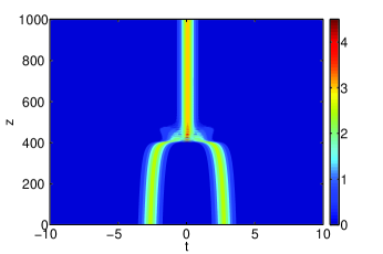
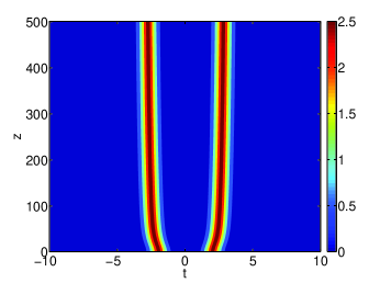
Figure 3: (Color online) Two pulse interaction when $\Delta\xi<d^{*}$. Initial pulses $(z=0)$ in phase: $\Delta\phi=0$, $\Delta\xi/\alpha\approx 7$ (top) merge while those out of phase by $\Delta\phi=\pi$ with $\Delta\xi/\alpha\approx 6$ (bottom) repel. Here $g=0.5$.

In the constant dispersion case this critical distance is found to be $\Delta\xi=d^{*}\approx 9\alpha$ (see Fig. 2) corresponding to soliton initial conditions. Interestingly, this is consistent with the experimental observations of Ref. [6]. To further illustrate, we plot the evolution of these cases in Fig. 3. At $z=500$ for the repelling solitons $\Delta\xi/\alpha=8.9$.

3 Perturbation theory

To obtain a more fundamental understanding of these numerical results we use perturbation theory to find evolution equations for the six parameters which define the interactions. These are: the pulse heights and velocities $\eta_{k}$ and $V_{k}$ respectively for $k=1,2$, the distance between pulse peaks $\Delta\xi$, and the difference in phase $\Delta\phi$. We take the subscripts 1 and 2 to denote the left and right pulse respectively and $\Delta\phi$ to be the phase of the right pulse minus that of the left pulse. Similarly, $\Delta\eta=\eta_{2}-\eta_{1}$ and $\Delta V=V_{2}-V_{1}$. Since the individual pulses are well approximated by solitons of the unperturbed NLS equation, the pulses are considered to be solutions of this equation which vary slowly under the perturbing effects of gain, loss, and filtering.

Let us denote the NLS equation with perturbation $F[\psi]$ as

$$i\psi_{z}+\frac{1}{2}\psi_{tt}+\left|\psi\right|^{2}\psi=F[\psi]$$ (2)

where

$$F[\psi]=\frac{ig}{1+\epsilon E}\psi+\frac{i\tau}{1+\epsilon E}\psi_{tt}-\frac{il}{1+\delta P}\psi$$

We write the four parameter family of soliton solutions to the unperturbed or classical NLS equation ($F=0$) as follows

$$\psi=ue^{i\phi},\quad u=\eta{\rm sech}(\eta\theta)$$ (3a)

$$\xi=\int_{0}^{z}Vdz+\xi_{0},\quad\theta=t-\xi,$$ (3b)

$$\sigma=\displaystyle\int_{0}^{z}(\mu+\frac{V^{2}}{2})dz+\sigma_{0},\quad\phi=V\theta+\sigma$$ (3c)

where $\mu$, $V$, $\xi_{0}$, $\sigma_{0}$ define height/width, speed, temporal shift and phase shift of the soliton respectively. For the classical NLS equation without gain, filtering and loss ($F=0$), $\mu$, $V$, $\xi_{0}$, $\sigma_{0}$ are constant. We also note that $\eta$ is directly related to $\mu$ by $\mu=\eta^{2}/2$. The effect of the right-hand-side being nontrivial is approximated by allowing $\mu$, $V$, $\xi_{0}$, $\sigma_{0}$ to vary slowly in $z$. The evolution of these parameters is found by satisfying the following integral conservation laws modified by $F[\psi]$ and derived from Eq. (2)

$$\frac{d}{dz}\int\left|\psi\right|^{2} =2\mathrm{Im}\int F[\psi]\psi^{*}$$ (4a)

$$\frac{d}{dz}\mathrm{Im}\int\psi\psi_{t}^{*} =2\mathrm{Re}\int F[\psi]\psi_{t}^{*}$$ (4b)

$$\frac{d}{dz}\int t\left|\psi\right|^{2} =-d_{0}\mathrm{Im}\int\psi\psi^{*}_{t}+2\mathrm{Im}\int tF[\psi]\psi^{*}$$ (4c)

$$\mathrm{Im}\int\psi_{z}\psi_{\mu}^{*} =-\frac{d_{0}}{2}\mathrm{Re}\int\psi_{t}\psi_{t\mu}^{*}+\mathrm{Re}\int\left|\psi\right|^{2}\psi\psi_{\mu}^{*}$$

$$\hskip 76.82234pt-\mathrm{Re}\int F[\psi]\psi_{\mu}^{*}$$ (4d)

where all integrals are taken over $-\infty<t<\infty$.

Along with the effects of gain, loss, and filtering, the effect of tail interaction between the two solitons is also treated as a perturbation. Since solitons are widely separated to leading order the full solution may be viewed as the superposition of two single solitons $\psi=\psi_{1}+\psi_{2}$; we take $\psi_{1}$ to be the soliton on the left and $\psi_{2}$ to be the soliton on the right. When $\psi_{1}$ is locally the dominant term $\psi_{2}$ is treated as a small parameter and we expand the nonlinear term about $\psi_{1}.$ If for the moment we omit the $F[\psi]$ term the evolution of $\psi_{1}$ is well approximated by

$$i\psi_{1z}+\frac{1}{2}\psi_{1tt}+\left|\psi_{1}\right|^{2}\psi_{1} =-2\left|\psi_{1}\right|^{2}\psi_{2}-\psi_{1}^{2}\ \psi_{2}^{*}$$

$$=G[\psi_{1},\psi_{2}]$$

and similarly an equation for when $\psi_{2}$ dominates is found to satisfy

$$i\psi_{2z}+\frac{1}{2}\psi_{2tt}+\left|\psi_{2}\right|^{2}\psi_{2} =-2\left|\psi_{2}\right|^{2}\psi_{1}-\psi_{2}^{2}\ \psi_{1}^{*}$$

$$=G[\psi_{2},\psi_{1}]$$

Notice that if $\psi_{1}$ and $\psi_{2}$ satisfy this system of coupled PDEs then their sum $\psi$ satisfies NLS. Any contributions from interaction in the gain, loss, and filtering terms would be a higher order term. For a more thorough treatment of this method for analyzing soliton interactions see Ref. [20] and for unperturbed NLS see Ref. [21]. Simplifications result if we assume that $\Delta V=V_{2}-V_{1}$ is small so that from the definition $\Delta\phi\approx-\bar{V}\Delta\xi+\Delta\sigma$. We also assume $\Delta\eta=\eta_{2}-\eta_{1}$ is small and approximate $\eta_{1}$ and $\eta_{2}$ as $\bar{\eta}$. For all variables the bar denotes the mean over the two solitons and $\Delta$ the difference of the right minus the left. These assumptions are all satisfied in the numerical simulations.

Including the perturbing terms $F$ we have a system of equations coupled in their perturbations as follows

$$i\psi_{1z}+\frac{1}{2}\psi_{1tt}+\left|\psi_{1}\right|^{2}\psi_{1}=G[\psi_{1},\psi_{2}]+F[\psi_{1}]$$

$$i\psi_{2z}+\frac{1}{2}\psi_{2tt}+\left|\psi_{2}\right|^{2}\psi_{2}=G[\psi_{2},\psi_{1}]+F[\psi_{2}]$$

both of which satisfy Eqs. (4). Substituting the soliton ansatz for $\psi_{1}$ and $\psi_{2}$ we find a system of first order differential equations for the slowly varying parameters $\eta_{k}$, $V_{k}$, $\xi_{0k}$, and $\sigma_{0k}$.

Subtracting the equations for $\frac{d\xi_{0k}}{dz}$, and $\frac{d\sigma_{0k}}{dz}$ we find

$$\frac{d\Delta\xi_{0}}{dz}=0,\quad\frac{d\Delta\sigma_{0}}{dz}=0$$

which means that $\Delta\xi_{0}$, $\Delta\sigma_{0}$ are stationary. Then, from Eqs. (3) we have $\Delta\phi\approx-\bar{V}\Delta\xi+\Delta\sigma$ and $\Delta\xi=\int_{0}^{z}(\Delta V)dz+\Delta\xi_{0}$ and by differentiating we arrive at the following approximate evolution equations

$$\frac{d\Delta\xi}{dz} =\Delta V+\Delta\xi_{0,z}=\Delta V$$

$$\frac{d\Delta\phi}{dz} =-\bar{V}_{z}\Delta\xi-\bar{V}\Delta\xi_{z}+\Delta\sigma_{z}$$

$$=-\bar{V}\Delta V+(\bar{\eta}\Delta\eta+\bar{V}\Delta V)+\Delta\sigma_{0,z}=\bar{\eta}\Delta\eta$$

The evolution equations are thus found to be

$$\frac{d\eta_{k}}{dz} =S_{1}(\eta_{k},V_{k})+(-1)^{k}4\bar{\eta}^{3}\sin(\Delta\phi)e^{-\bar{\eta}\Delta\xi}$$ (5a)

$$\frac{dV_{k}}{dz} =S_{2}(\eta_{k},V_{k})+(-1)^{k+1}4\bar{\eta}^{3}\cos(\Delta\phi)e^{-\bar{\eta}\Delta\xi}$$ (5b)

$$\frac{d\Delta\xi}{dz} =\Delta V$$ (5c)

$$\frac{d\Delta\phi}{dz} =\bar{\eta}\Delta\eta$$ (5d)

where

$$S_{1}(\eta,V,\bar{\eta}) =g\left(\frac{2\eta}{E_{0}+1}\right)-\tau\frac{1}{E_{0}+1}\left(\frac{2}{3}\eta^{3}+2V^{2}\eta\right)$$

$$\hskip 56.9055pt+l\left[2\eta\frac{1}{a-b}\log\left(\frac{a}{b}\right)\right]$$

$$S_{2}(\eta,V,\bar{\eta}) =-\tau V\left(\frac{4}{3}\frac{\eta^{2}}{E_{0}+1}\right)$$

Here $a$ and $b$ are the complex conjugate roots of the polynomial $x^{2}+2(1+2\eta^{2})x+1=0$. The energy for the two NLS solitons is $E_{0}=4\bar{\eta}$. Note $a$ and $b$ can be chosen to be either root of the quadratic equation. A more detailed derivation of these equations may be found in [22, 23], along with an analysis of how interactions of solitons in Eq. (1) differ from those in the unperturbed NLS equation. A comparison of the numerical results to those found from the asymptotic analysis are seen in Fig. 4 for initial conditions $\eta_{10}=\eta_{20}=3.3$, $\Delta\xi_{0}=3$ ($\Delta\xi_{0}/\alpha=6$), and $\Delta\phi_{0}=3\pi/4$.

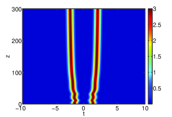
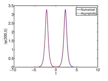
Figure 4: (Color online) Numerical simulation (top), asymptotic analysis (middle) and comparison of the numerical simulation and the asymptotic result at $z=300$ (bottom). Here $g=0.6$.

In Eqs. (5) the terms $S_{1}$ and $S_{2}$ are the contributions from gain, loss and filtering, while the other terms come from the tail interactions. Considering just the effects of gain, loss and filtering, the velocities have a single stable equilibrium $V_{1}=V_{2}=0$ for any positive value of $\eta_{1}$ and $\eta_{2}$ (negative values of $\eta_{1}$ or $\eta_{2}$ are only a phase shift from their positive counter parts), so we look at the dynamics of $\eta_{1}$ and $\eta_{2}$ for $V_{1}$ and $V_{2}$ at this equilibrium. Fig. 5 shows the phase plane for gain values above and below the threshold for stable two pulse solutions. In both cases there exists a stable equilibrium at $\eta_{k}=0$ for $k=1$ or $2$ which amounts to a reduction to the single soliton case and an unstable equilibrium when both $\eta_{1}=\eta_{2}=0$ for any $g>l$. Also, in both cases we see an equilibrium at $\eta_{1}=\eta_{2}=\eta^{*}$, however, for $g<g_{c}$ it is found to be unstable and for $g>g_{c}$, it is stable; $g_{c}\approx 0.45.$

In Fig. 5 typical cases are shown. Here $g=0.4$ (top) is unstable and $g=0.6$ (bottom) is stable. The $\eta^{*}$ found from perturbation theory agrees with the height found numerically to several decimal places. We also note that there are two other two equilibria found for $g=0.6$ which are unstable.

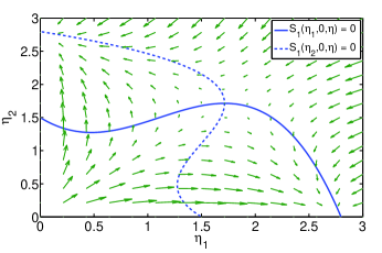
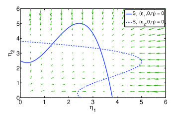
Figure 5: (Color online) Typical phase planes for $\frac{d\eta_{1}}{dz}$ and $\frac{d\eta_{2}}{dz}$ with $V_{1}=V_{2}=0$ for the unstable two soliton case, $g=0.4$ (top) and the stable two soliton case, $g=0.6$ (bottom).

When the soliton interaction terms are taken into consideration, $S_{1}$ and $S_{2}$ are found to still be the dominant terms for sufficiently large $\Delta\xi,$ hence $\eta_{k}\rightarrow\eta^{*}$ and $V_{k}\rightarrow 0$ for $k=1,2$. However, the small contributions from the interaction terms can cause small decaying oscillations for large $z.$ Solving the perturbation theory derived system, we find a stable equilibrium at $\Delta\phi=\pi$ for any $\eta$ as well as an unstable equilibrium for $\Delta\phi=0$ and $\Delta\eta=0$. See typical cases in Fig. 6. The peak separation is further characterized by the phase difference; the pulses attract each other when $-\pi/2\leq\Delta\phi<\pi/2$ and repel when $\pi/2<\Delta\phi\leq 3\pi/2$. This is seen from inspecting the sign of $\Delta V_{t}=-8\bar{\eta}^{3}\cos(\Delta\phi)\exp(\bar{\eta}\Delta\xi)$ for two solitons with zero velocity. Thus, for initial phase difference $\Delta\phi_{0}=0$ the pulses will eventually collide and combine into a single pulse, while for $\Delta\phi_{0}\neq 0$ the phase difference will evolve to $\pi$ and after some initial oscillations the pulses will repel.

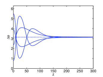
Figure 6: (Color online) Evolution of the phase for $\eta_{10}=\eta_{20}=3.3$, $\Delta\xi_{0}=3.0$ ($\Delta\xi_{0}/\alpha\approx 6$) and several choices of initial phase difference. Here $g=0.6$. $\Delta\phi=\pi$ is shown with a dashed line.

There is not a non-trivial equilibrium for the full Eqs. (5), so the “effective high order soliton state found numerically is not a “true” bound state. We will show, however, that $\Delta\xi(z)=O(\log(z))$ so once the solitons are a certain distance $d^{*}$ apart they will be moving too slowly to see or measure. By comparison, for the classical NLS equation $\Delta\xi(z)=O(z)$ [21]. This difference is illustrated in Fig. 7 for $\Delta\phi_{0}=\pi/4$. These “effective” bound states emerge naturally from the interaction of pulses for most initial conditions making them attractors of Eq. (1).

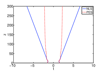
Figure 7: (Color online) Comparison of NLS to PES; initially the solitons have $\Delta\phi=\pi/4$. For Eq. (1) the resulting pulses have phase difference $\Delta\phi=\pi$. Here $g=0.6$.

Using the fact that $\eta_{1}=\eta_{2}\rightarrow\eta^{*}$ and $\Delta\phi\rightarrow\pi$ as $z\rightarrow\infty$ we can derive the asymptotic behavior of $\Delta\xi$. First we take the difference of $\frac{dV_{2}}{dz}$ and $\frac{dV_{1}}{dz}$ and the derivative of $\frac{d\Delta\xi}{dz}$ giving us

$$\frac{d\Delta V}{dz} =-\tau\left(\frac{4}{3}\frac{\eta^{*2}}{4\eta^{*}+1}\right)\Delta V+8\eta^{*3}e^{-\eta^{*}\Delta\xi}$$

$$\frac{d^{2}\Delta\xi}{dz^{2}} =\frac{d\Delta V}{dz}$$

which may now be combined to form a second order differential equation for $\Delta\xi$

$$3\frac{d^{2}}{dz^{2}}\Delta\xi=-\tau\left(\frac{4}{3}\frac{\eta^{*2}}{4\eta^{*}+1}\right)\frac{d}{dz}\Delta\xi+8\eta^{*3}e^{-\eta^{*}\Delta\xi}=0$$

Since the evolution of $\Delta\xi$ is seen from numerical simulations to be evolving slowly in $z$ we expect that $\frac{d^{2}}{dz^{2}}\Delta\xi\ll\frac{d}{dz}\Delta\xi$ and so $\frac{d^{2}}{dz^{2}}\Delta\xi$ can be neglected as being a higher order term. This leaves a first order equation which we solve to get the long term behavior of $\Delta\xi$ to be

$$\Delta\xi \rightarrow \frac{1}{\eta^{*}}\log\left[\frac{6\eta^{*}(1+4\eta^{*})}{\tau}z\right]$$

In fact it is found numerically that the divergence is considerably less than $\log z$. Hence we call these higher states “effectively bound” because in practice the laser propagation distance is bounded.

As mentioned above, by increasing the gain parameter additional pulses may be supported. In this way we can find three and four soliton states that emerge from unit gaussian initial states as shown in Fig. 8. In all cases pulses of height $\eta^{*}$ were taken at an initial separation of $\Delta\xi=9\alpha$ and evolved to $z=1000$ with less then $0.1$ change in peak positions.

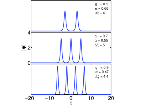
Figure 8: (Color online) Multiple high-order bound state soliton solutions of the anomalously dispersive PES model.

The depicted solitons are all in phase, however such higher order states can be found for any choice of (initial) pair wise phase differences. Interestingly, for no interactions to occur the critical separation distance between the solitons is again found to be $d^{*}\approx 9\alpha$ for the three and four soliton states. For $\Delta\xi<d^{*}$ the interactions of three and four solitons are more varied, but essentially result in either evolving to a lower state through the merging of pulses or pulses repelling each other beyond the critical distance $d^{*}$. This behavior agrees with what was found for the two soliton state.

4 Normal Higher Order Solitons

Next we briefly mention some results for the constant normal dispersive case: $d_{0}=-1<0$. As mentioned above, individual pulses of Eq. (1) in the normal regime exhibit strong chirp and cannot be identified as the solutions of the “unperturbed” NLS equation. Indeed, the classical NLS equation does not exhibit decaying “bright” soliton solutions in the normal regime. If we begin with an initial gaussian, $\psi(0,t)=\exp(-t^{2})$, the evolution mode-locks into a fundamental soliton state; see Fig. 1 bottom two figures. These figures clearly exhibit the mode-locking evolution and the significant chirp of the pulse. On the other hand we can obtain a higher-order anti-symmetric soliton, i.e. an anti-symmetric bi-soliton, one which has its peaks amplitudes differing in phase by $\pi$. Such a state can be obtained if we start with an initial state of the form $\psi(0,t)=t\exp(-t^{2})$ (i.e. a Gauss-Hermite polynomial). The evolution results in an anti-symmetric bi-soliton and is shown in Fig. 9 along with a comparison to the profile of the single soliton. This is a true bound state. Furthermore, the results of our study finding anti-symmetric solitons in the normal regime are consistent with recent experimental observations [8].

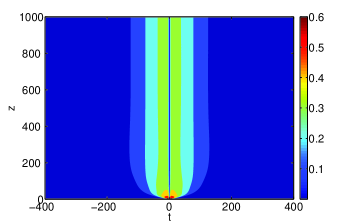
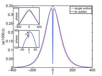
Figure 9: (Color online) Evolution of the anti-symmetric soliton (top) and the anti-symmetric (bi-soliton) superimposed with the relative single soliton (bottom) at $z=1000$. Here $g=1.5$.

It is interesting that the normal regime also exhibits higher soliton states when two general initial pulses (e.g. unit gaussians) are taken sufficiently far apart. The resulting pulses, shown in Fig. 10, individually have a similar shape to the single soliton of the the normal regime with lower individual energies. These pulses if initially far enough apart can have independent chirps which may be out of phase by an arbitrary constant. We again find that $d^{*}\approx 9\alpha$ is a good estimate for the required pulse separation just as in the constant anomalous dispersive case! These pulses are “effective bound states” in that after a long distance they separate very slowly (too slowly to measure).

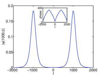
Figure 10: (Color online) Symmetric two soliton state of the normal regime with in phase pulses. The phase structure is depicted in the inset. Here $g=1.5.$

Additional higher order $3,4,...$ soliton states can also be found. We will not go into further details here.

5 Dispersion managed systems

Standard dispersion managed (DM) solitons, like their constant dispersive counterparts, are obtained from the PES model over a wide range of anomalous dispersion [15]. This is important since recent mode-locked laser experiments have been conducted in dispersion-managed regimes [13, 8, 17]. In correspondence with Ti:Sapphire DM laser systems we allow the dispersion to vary in $z$ as well as introducing nonlinear management in the form of the function $n(z)$ multiplying the nonlinear term. Equation (1), is used but we change the symbol of the envelope from $\psi=\psi(z,t)$ to $u=u(z,t)$ to distinguish the two cases (constant dispersion and DM, respectively). The effect of dispersion management is obtained by splitting the dispersion $d(z)$ into two components $d(z)=d_{0}+\Delta(z/z_{\alpha})/z_{\alpha}$ where $0<z_{\alpha}<<1$ is the dispersion-map period. Hence $d(z)$ is large and periodic. If $d(z)$ was only $O(1)$ then the multi-scale averaging method employed below would result in the constant dispersive case discussed earlier. The path averaged dispersion is $d_{0}$ and $\Delta(z/z_{\alpha})$ is a rapidly varying function with zero average which we define as follows: $\Delta(\zeta)=\{-\Delta_{1},0<\zeta<1/2;\Delta_{2},1/2<\zeta<1\}$. Here we consider the case of positive average dispersion $(d_{0}>0)$. We define the map strength $s=\Delta_{1}/2$ which gives a measure of the variability of dispersion around the average. We take $d_{0}=1,z_{a}=0.1$ and vary $s$. The effect of the nonlinear management is to turn the nonlinearity “off and on”, i.e. $n(\zeta)=\{0,0<\zeta<1/2;1,1/2<\zeta<1\}$. For example, in a Ti:Sapphire laser the nonlinearity is negligible in the anomalous regime where one has a prism pair that compensates for the normal dispersion in the crystal. The averaged equation is derived using the method of multiple scales and perturbation theory [24]. The variation in dispersion occurs on the short distance scale $\zeta=z/z_{\alpha}$ and the pulse envelope evolves on the long scale $Z=z$.

The method proceeds by expanding $u$ in powers of $z_{\alpha}$:

$$u(\zeta,Z,t)=u^{(0)}(\zeta,Z,t)+z_{\alpha}u^{(1)}(\zeta,Z,t)+O(z_{\alpha}^{2})$$

and substituting this into Eq. (1) to obtain a series of equations by relating terms by powers of $z_{\alpha}$. At $O(z_{\alpha}^{-1})$

$$i\frac{\partial u^{(0)}}{\partial\zeta}+\frac{\Delta(\zeta)}{2}\frac{\partial^{2}u^{(0)}}{\partial t^{2}}=0$$

which can be solved using Fourier transforms to arrive at

$$\hat{u}^{(0)}(\zeta,Z,\omega)=\hat{U}_{0}(Z,\omega)\exp\left[-i\frac{\omega}{2}C(\zeta)\right]$$

where $C(\zeta)=\int_{0}^{\zeta}\Delta(\zeta^{\prime})d\zeta^{\prime}$, $\hat{U}_{0}(Z,\omega)=\hat{u}^{(0)}(\zeta=0,Z,\omega)$, and the Fourier transform pair is defined as

$$\hat{u}(\omega)=\mathcal{F}\{u(t)\} =\int_{-\infty}^{+\infty}u(t)e^{i\omega t}dt$$

$$u(t)=\mathcal{F}^{-1}\{\hat{u}(\omega)\} =\frac{1}{2\pi}\int_{-\infty}^{+\infty}\hat{u}(\omega)e^{-i\omega t}d\omega$$

Thus $\hat{u}_{0}$ separates into a slowly evolving envelope $\hat{U}_{0}$ and fast oscillations due to changes in the local dispersion. The equation for $\hat{U}_{0}$ is obtained by imposing secularity conditions on the $O(1)$ terms,

$$i\frac{\partial\hat{U}_{0}}{\partial Z}-\frac{d_{0}}{2}\omega^{2}\hat{U}_{0} +\displaystyle\int_{0}^{1}\exp\left[-i\frac{\omega}{2}C(\zeta)\right](\mathcal{F}\{|u^{(0)}|^{2}u{(0)}\}$$

$$-\mathcal{F}\{F[u^{(0)}]\})d\zeta=0,$$ (6)

This is the averaged, or mean-field equation which we solve to find the pulse dynamics. In the case where $F=0$ this is known as the dispersion managed NLS or DMNLS equation [24].

The method of spectral renormalization [25] can be employed to find single mode-locked DM solitons for Eq. (6) [15]. Here we initially superimpose two such DM soliton pulses at varying peak separations with phase difference $\Delta\phi=0$ and let them evolve to find two soliton “effective” bound states. As a criterion for an “effective” bound state, we require the the peak separation differ less than $0.05\alpha$ after evolving $500$ units in $z$. Typical examples with comparison of initial vs. final states are depicted in Figs. 11 and 12. Much like the single soliton case the individual pulses are well approximated by the solutions of the unperturbed DMNLS equation. We also note that due to the nonlocality of the equation, the individual pulses have a smaller energy than the single pulse for the same parameters, as was in the case of constant dispersion.

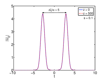
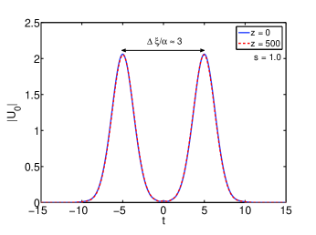
Figure 11: (Color online) “Effective” bound state for two solitons in DM system for $s=0.$ (top) and $s=1.0$ (bottom). Here $g=0.6$.

As is indicated in the figure, the minimum initial distance $d^{*}\approx 9\alpha$ no longer holds for the dispersion (and nonlinearly) managed PES equation (DMPES). In the nonlinear managed system we find that the critical distance $d^{*}\approx 7\alpha$ for $s=0$, i.e. constant dispersion, and $d^{*}$ depends on the map strength $s$ for $s>0$. Since this change is much more dramatic between $s=0$ and $s=1$ than $s=1$ and $s=10$ we investigate this region more thoroughly. In Fig. 12 the value of $\Delta\xi/\alpha$ found for the pulses to be “effectively” bound are plotted for varying map strengths. The general trend is for the needed separation to decrease as $s$ increases, however, as can be seen between $s=0.1$ and $s=1.0$ where more $s$ values were tested this is not a monotonically decreasing process.

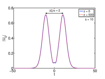
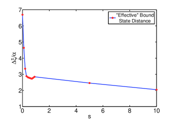
Figure 12: (Color online) “Effective” bound state for two solitons in DM system for $s=10$ (top). Numerically found relation between the map strength $s$ and the minimum initial distance $\Delta\xi_{0}/\alpha$ for no interactions to be seen (bottom) after $z=500$ units. Here $g=0.6$.

For more information on the normal ($d_{0}<0$) DM case we refer the reader to Ref. [19].

6 Anti-Symmetric Bi-Solitons for DM Systems

We now superimpose two net anomalous DM solitons with a $\pi$ phase difference. For $s<s_{*}\approx 0.25$ pulses repel each other as was the case for constant anomalous dispersion; we note that for the above values of the map strength both of the local dispersions being used ($d_{0}+\Delta_{1}/z_{a}$ and $d_{0}+\Delta_{2}/z_{a}$) are in the anomalous regime. For $s>s_{*}$, pulses which are taken close enough together, i.e. the distance between peak values, $d<d_{*}\approx 2.5,$ are found to lock into a bi-soltion state. Examples are given in Fig. 13. Pulses taken further apart: $d>d_{*}$ are found to repel. These anti-symmetric bi-solitons are the mode-locked (due to gain-loss) analog of what was obtained in the case of pure DM systems without gain loss [26, 27].

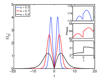
Figure 13: (Color online) Bi-Soltion states found for $s=0.3,0.7$ and 5.0. Here $g=0.6$. The relative phases and the $\pi$ jumps at the origin are shown in the insets.

7 Summary

To conclude, we investigated Eq. (1) and found a large class of localized solutions including: mode-locked solitons in both the constant anomalous and normal regimes, high-order solitons in the constant anomalous regime and anti-symmetric bi-solitons in the constant normal regime. These results are consistent with experimental observations of higher-order solitons in the anomalous and bi-solitons in the normal dispersive regimes. The dispersion and nonlinear managed system was also investigated. Here in the averaged anomalous regime single and higher-order soliton pulses were obtained, including anti-symmetric bi-solitons in the net anomalous regime. For the constant dispersion case, it is found that when individual pulses are initially separated by $d^{*}\approx 9\alpha$ where $\alpha$ is the width of the individual pulse the result is a soliton string. For the DM system the results indicate that the high-order soliton strings in the DM case can exist in much closer proximity to each other.

References

- [1] H. Haus, Mode-locking of lasers, IEEE J. Sel. Topics Q. Elec. 6 (2000) 1173–1185.
- [2] J. Ye, S. Cundiff, Femtosecond optical frequency comb: Technology, principles, operation & application, Springer, 2005.
- [3] M. Fischer, N. Kolachevsky, M. Zimmermann, R. Holzwarth, T. Udem, T. Hänsch, M. Abgrall, J. Grüunert, I. Maksimovic, S. Bize, H. Marion, F. P. D. Santos, P. Lemonde, G. Santarelli, P. Laurent, A. Clairon, C. Salomon, M. Haas, U. Jentschura, C. Keitel, New limits on the drift of fundamental constants from laboratory measurements, Phys. Rev. Lett. 92 (2004) 230802.
- [4] W.E. Lamb Jr., Theory of an optical laser, Phys. Rev. 134 (1964) A1429–Al450.
- [5] H. Haus, J. Fujimoto, E. Ippen, Analytic theory of additive pulse and kerr lens mode locking, IEEE J. Quant. Elec. 28 (1992) 2086–2096.
- [6] D. Tang, W. Man, H. Tam, P. Drummond, Observation of bound states of solitons in a passively mode-locked fiber laser, Phys. Rev. A 64 (2001) 033814.
- [7] P. Grelu, F. Belhache, F. Gutty, J. Soto-Crespo, Phase-locked soliton pairs in a stretched-pulse fiber laser, Opt. Lett. 27 (2002) 966–968.
- [8] A. Chong, W. Renninger, F. Wise, Observation of antisymmetric dispersion-managed solitons in mode-locked laser, Opt. Lett. (to appear).
- [9] J. Kutz, Mode-locked soliton lasers, SIAM Rev. 48 (2009) 629–678.
- [10] T. Kapitula, J. Kutz, S. B., Stability of pulses in the master mode-locking equation, J. Opt. Soc. Am. B 19 (2002) 740–746.
- [11] N. Akhmediev, A. Ankiewicz, Generation of a train of solitons with arbitrary phase difference between neighboring solitons, Opt. Lett 19 (1994) 545–547.
- [12] N. Akhmediev, A. Ankiewicz, J. Soto-Crespo, Stable soliton pairs in optical transmission lines and fiber lasers, J. Opt. Soc. Am. B 15 (1998) 515–523.
- [13] F. O. Ilday, J. R. Buckley, W. G. Clark, F. W. Wise, Self-similar evolution of parabolic pulses in a laser, Phys. Rev. Lett. 92 (2004) 213902.
- [14] Q. Quraishi, S. Cundiff, B. Ilan, M. Ablowitz, Dynamics of nonlinear and dispersion managed solitons, Phys. Rev. Lett. 94 (2005) 243904.
- [15] M. Ablowitz, T. Horikis, B. Ilan, Solitons in dispersion-managed mode-locked lasers, Phys. Rev. A 77 (2008) 033814.
- [16] M. Ablowitz, T. Horikis, Pulse dynamics and solitons in mode-locked lasers, Phys. Rev. A 78 (2008) 011802(R).
- [17] M. Sanders, J. Birge, A. Benedick, H. Crespo, F. Kärtner, Dynamics of dispersion-managed octave-spanning titanium: sapphire lasers, J. Opt. Soc. Am. B 26 (2006) 743–749.
- [18] F. Ilday, F. Wise, F. Kaertner, Possibility of self-similar pulse evolution in a ti:sapphire laser, Opt. Express 12 (2004) 2731–2738.
- [19] M. Ablowitz, T. Horikis, Soliton pulses in normally dispersive mode-locked lasers, Preprint, 2009.
- [20] V. Karpman, V. Solov’ev, A perturbation theory for soliton systems, Physica D 3 (1981) 142–164.
- [21] Y. Zhu, J. Yang, Universal fractal strcutures in the weak interaction of solitary waves in generalized nonlinear schrodinger equations, Phys. Rev. E 75 (2007) 036605.
- [22] M. Ablowitz, T. Horikis, S. Nixon, Y. Zhu, Asymptotic analysis of pulse dynamics in mode-locked lasers, Stud. Appl. Math. 122 (2009) 411–425.
- [23] S. Nixon, Mathematical analysis of nonlinear optical phenomena, Ph.D. thesis, University of Colorado (2010).
- [24] M. Ablowitz, G. Biondini, Multiscale pulse dynamics in communication systems with strong dispersion management, Opt. Lett. 23 (1998) 1668–1670.
- [25] M. Ablowitz, Z. Musslimani, Spectral renormalization method for computing self-localized solutions to nonlinear systems, Opt. Lett. 30 (2005) 2140–2142.
- [26] A. Maruta, T. Inoue, Y. Nonaka, Y. Yoshika, Bisoliton propagating in dispersion-managed system and its application to high-speed and long-haul optical transmission, IEEE J. Sel. Top. Quantum Electron. 8 (2002) 640–650.
- [27] M. Ablowitz, T. Hirooka, T. Inoue, Higher-order asymptotic analysis of dispersion-managed transmission systems: solutions and their characteristics, J. Opt. Soc. Am. B 19 (2002) 2876–2885.