Dynamics of Scalar Field Dark Matter With a Cosh-like Potential

Abstract

The dynamics of a cosmological model fueled by scalar field dark matter with a cosh-like potential plus a cosmological constant is investigated in detail. It is revealed that the late-time attractor is always the de Sitter solution, and that, depending on the values of the free parameters, the oscillating solution of the scalar field – modeling cold dark matter – mediates between some early stage (say, the radiation-dominated solution) and the accelerating de Sitter attractor.

I Introduction

One of the greatest mysteries of modern Cosmology doubtless is the nature of dark matter (DM) (for a review seeDMreviw ). We know that more than 23% of the matter of the universe is attractive, but of unknown nature. The most accepted candidate are particles from the Minimal Supersymmetric Standard Model (MSSM)MSSMreview . This paradigm has been proved at cosmological level with a great success. For example, it predicts very well the formation and clustering of galaxiesStForreview , and the micro-Kelvin temperature fluctuations of the cosmic microwave background (CMB) of the universeCMBreview . These two predictions represent the main achievements of the model.

Nevertheless, in the last decade, some inconsistencies of the model when calcullations are compared with the observations at galactic level, have arosen. For example, amongst other problems, the predicted number of satellite galaxies around big galaxies is much bigger than the observed onesatelites , and the DM density profile at the center of galaxies seems to be steeper than observedcusp .

Even though there have been several attempts to deal with these inconsistenciesinconsist , one compelling possibility is the hypothesis that the DM is a scalar field, more than a Standard Model (SM) particlel9 . The idea is rooted on the fact that almost all the unified theories of physics contain scalar fields as the simplest geometrical objects. These scalar fields are often called Higgs, Inflatons, Dilatons, Scalerons, Radions, etc. All of them are needed to achieve mathematical and physical consistency of these theories. With the discovery of the dark energy (DE), attempts to relate scalar fields with the DE also have had some success (seeCopeland:2006wr for a comprehensive review).

In Ref. l9 some of us proposed that a scalar field rolling down a convex self-interaction potential can be a reasonable candidate for DM, calling this hypothesis as Scalar Field Dark Matter (SFDM). This hypothesis has some nice features. For example, the SFDM does not need extra hypothesis to explain the flat DM profile in the center of galaxiesargelia , or the number of satellite galaxies around the Milky Wayfurther .

The SFDM hypothesis has been investigated for a number of self-interaction potentials like the cosh-like wang ; mul ; tona , and the quadratic ones tona ; quad , with the consequent discovery of several exact solutions of cosmological interest. However, within the cosmological context, a full and detailed study of the dynamics of SFDM models, to uncover their relevant asymptotic properties, is still desirable.

The main goal of the present paper is, precisely, to study within the cosmological context and by means of the dynamical systems tools, the asymptotic properties of the SFDM model driven by a cosh-like potential. Several relevant cosmological solutions will be correlated with such important dynamical systems concepts like past and future attractors, signaling the way the cosmic dynamics transits from early-time to intermediate and then to late-time asymptotic states.

It will be demonstrated, in particular, that the SFDM model driven by a cosh-like potential with a cosmological constant term added, is a good candidate to correctly describe a cosmic dynamics whose fate is, eventually, the inflationary de Sitter regime that can be correlated with present accelerated stage of the expansion of the Universe. Due attention will be paid to the late-time oscillatory solution that can e associated with cold dark matter (CDM) behaviour in the model, and that, inevitably, leads to the inflationary de Sitter attractor.

The paper has been organized as it follows. The relevant physical features of the model are discussed in the next section, and then, in section III, its mathematical features are specified. The details of the (linear) dynamical systems study of the SFDM model with a cosh-like potential, are given in section IV. The main results of the study are summarized in section V. Finally, in section VII, the physical discussion of the results and brief conclusions of the study are provided. We use the natural system of units where $\kappa^{2}=8\pi G=c=1$.

II Scalar Field Model with a cosh-like Potential

In a cosmological context, scalar fields with a cosh-like self-interaction potential have been studied, for instance, inwang . In that reference the following potential was investigated:

$$V(\phi)=V_{0}[\cosh(\lambda\phi)-1]^{\beta}\,,$$ (1)

where $\lambda$ and $\beta$ are free parameters. It was shown, see alsoTurner:1983he , that during the oscillatory phase the virial theorem gives the following expression for the mean equation of state:

$$\left\langle\omega_{\phi}\right\rangle=\left\langle\frac{\dot{\phi}^{2}-2V}{\dot{\phi}^{2}+2V}\right\rangle=\frac{\beta-1}{\beta+1}\,.$$ (2)

In consequence, for $\beta=1$ the scalar field behaves like pressureless dust $\left\langle\omega_{\phi}\right\rangle=0$. A scalar field potential with this value of $\beta$ could therefore play the role of cold dark matter in the universe. For $\beta<1/2$ this potential is a good candidate for the quintessence insteadwang .

In this paper we will focus our attention, precisely, in a cosh-like potential(1) with $\beta=1$ with a cosmological constant term added to it. The latter ingredient is neccessary to include dark energy in the model, as long as oscillations of the scalar field around the minimum of $\cosh$-potential play the role of the CDM (in fact SFCDM).

A reasonable physical assumption for the initial conditions is that the energy density in the scalar field was comparable to that of radiation at very early times, say, at the end of inflation wang . At such early times, the large value of $\phi$ makes the cosh-like potential(1) behave as an exponential one of the form $V(\phi)\propto\exp(-\beta\lambda\phi)$, and the scalar field energy density decreases rapidly so that it remains subdominant until recently.

In later times the form of $V(\phi)$ changes to a power law, resulting in rapid oscillations of the scalar ield around $\phi=0$. At this stage the scalar field equation of state mimics that of CDM in agreement with the present cosmological standard model paradigm. Due to the addition of the cosmological constant term, the resulting picture does indeed represent a unification of the dark matter and the dark energy. The present model might be called $\Lambda$-SFCDM.

The goal of this paper will be to describe the dynamical picture produced by the cosh-like potential (1) with $\beta=1$ and with the addition of a cosmological constant term, to put the above physical discussion on solid dynamical systems grounds.

III Mathematical Features of the Model

In this paper we focus in a Friedmann-Robertson-Walker space-time with flat spatial sections, filled with a mixture of two fluids: i) a perfect fluid of ordinary matter with density $\rho_{\gamma}$ and barotropic index $0\leq\gamma\leq 2$ ($\gamma=1$ for dust, $\gamma=4/3$ for radiation, etc.), and ii) a united $\Lambda$-SFCDM component with energy density $\rho_{\phi}=\dot{\phi}^{2}/2+V(\phi)$ and parametric pressure $p_{\phi}=\dot{\phi}^{2}/2-V(\phi)$. The relevant cosmological equations of the model are the following

$$\dot{H} = -\frac{1}{2}\left(\dot{\phi}^{2}+\gamma\rho_{\gamma}\right)\,,$$ (3a)

$$\ddot{\phi} = -3H\dot{\phi}-\frac{dV}{d\phi}\,,$$ (3b)

$$\dot{\rho}_{\gamma} = -3H\gamma\rho_{\gamma}\,,$$ (3c)

plus the Friedmann constraint:

$$H^{2}=\frac{1}{3}\left(\rho_{\gamma}+\frac{1}{2}\dot{\phi}^{2}+V\right)\,.$$ (4)

As anticipated, here we deal with a cosh-like potential of the form

$$V(\phi)=V_{0}[\cosh(\lambda\phi)-1]+\Lambda\,,$$ (5)

where $\Lambda\geq 0$ is a positive cosmological constant, and the parameter $\lambda$ is also a possitive quantity ($\lambda>0$). As it has been discussed in the former section, the potential $V(\phi)$ in (5) comprises both CDM and dark energy in a united ansatz. Actually, for a vanishing $\Lambda=0$, this potential is a particular case of (1), when the free parameter $\beta=1$, meaning that, once the oscillatory phase is attained, the scalar field driven by the potential (5) behaves like dust, i. e., just like CDM (see equation (2)). Since in this model $\Lambda\neq 0$, the scalar field energy density performs damped oscillations around $V_{min}=\Lambda$, meaning that the CDM energy density – accounted for by the oscillatory component – decreases until, eventually, the cosmological constant component dominates.

The potential $V(\phi)$ in (5) is a minimum at $\phi=0,\;\Rightarrow\;V_{min}=V(0)=\Lambda$. Additionally, in a natural scenario for the cosmic dynamics driven by $V(\phi)$, the scalar field $\phi$ runs from arbitrarily large negative values ($|\phi|\gg 1$), to vanishing ones ($|\phi|\ll 1$). In consequence, at early times the dynamics is driven by an exponential potential

$$|\phi|\gg 1/\lambda\;\;\Rightarrow\;\;V(\phi)\approx\bar{V}_{0}\;e^{-\lambda\phi},\;\;\bar{V}_{0}\equiv\frac{V_{0}}{2}\,,$$ (6)

whereas at late times it is associated with a power-law potential plus a cosmological constant:

$$|\phi|\ll 1/\lambda\;\;\Rightarrow\;\;V(\phi)\approx\frac{m^{2}}{2}\phi^{2}+\Lambda,\;\;m^{2}\equiv V_{0}\lambda^{2}\,.$$ (7)

The latter is just the quadratic potential that has been formerly studied, for instance, in references tona ; quad .

IV Dynamical Systems Study

The dynamical systems tools offer a very useful approach to the study of the asymptotic properties of the cosmological models coley ; Copeland:2006wr . In order to be able to apply these tools one has to (unavoidably) follow the steps enumerated below.

• First: to identify the phase space variables that allow writing the system of cosmological equations in the form of an autonomus system of ordinary differential equations (ODE). There can be several different possible choices, however, not all of them allow for the minimum possible dimensionality of the phase space.

• Next: with the help of the chosen phase space variables, to build an autonomous system of ODE out of the original system of cosmological equations.

• Finally (some times a forgotten or under-appreciated step): to indentify the phase space spanned by the chosen variables, that is relevant to the cosmological model under study.

After this recipe one is ready to apply the standard tools of the (linear) dynamical systems analysis.

IV.1 Autonomous System of ODE

Let us to introduce the following dimensionless phase space variables in order to build an autonomous system out of the system of cosmological equations (3c) and (4)wands

$$x\equiv\frac{\dot{\phi}}{\sqrt{6}H},\;y\equiv\frac{\sqrt{V}}{\sqrt{3}H}\,.$$ (8)

After this choice of phase space variables we can write the following autonomous system of ordinary differential equations

$$x^{\prime} = -\sqrt{\frac{3}{2}}\frac{\partial_{\phi}V}{V}y^{2}-3x+\frac{3}{2}x(2x^{2}+\gamma\Omega_{\gamma})\,,$$ (9a)

$$y^{\prime} = \sqrt{\frac{3}{2}}\frac{\partial_{\phi}V}{V}xy+\frac{3}{2}y(2x^{2}+\gamma\Omega_{\gamma})\,,$$ (9b)

where a prime denotes derivative with respect to the time variable $\tau\equiv\ln a$ (properly speaking the number of e-foldings of expansion), and the dimensionless density parameter $\Omega_{\gamma}\equiv\rho_{\gamma}/3H^{2}$ is given through the following expression

$$\Omega_{\gamma}=1-x^{2}-y^{2}\,,$$ (10)

which is just a rewriting of the Friedmann constraint (4).

As long as one considers just constant and exponential self-interaction potentials ($\partial_{\phi}V=0$ and $\partial_{\phi}V=\rm{const}$, respectively), Eqs. (9a) and (9b) form a closed autonomous system of ODE. However, if one wants to go further and to consider a wider class of self-interaction potentials beyond the exponential one – as it is the case in the present study –, the system of ODE (9a) and (9b) is not a closed system of equations any more, since, in general, $\partial_{\phi}V$ is a function of the scalar field $\phi$.

A way out of this difficulty can be based on the method developed in chinos . In order to be able to study arbitrary self-interaction potentials one needs to consider one more variable $v$, that is related with the derivative of the self-interaction potential through the following expression

$$v\lambda\equiv-\partial_{\phi}V/V=-\partial_{\phi}\ln V\,.$$ (11)

Hence, an extra equation

$$v^{\prime}=-\sqrt{6}\lambda xv^{2}(\Gamma-1)\,,$$ (12)

has to be added to the above autonomous system of equations. The quantity $\Gamma\equiv V\partial_{\phi}^{2}V/(\partial_{\phi}V)^{2}$ in Eq. (12) is, in general, a function of $\phi$. The idea behind the method inchinos is that $\Gamma$ can be written as a function of the variable $v$, and, perhaps, of several constant parameters. Indeed, for a wide class of potentials the above requirement – $\Gamma=\Gamma(v)$ –, is fulfilled.

Let us introduce a new function $f(v)=v^{2}(\Gamma(v)-1)$ so that Eq.(12) can be written in the more compact form

$$v^{\prime}=-\sqrt{6}\lambda xf(v)\,.$$ (13)

Eqs. (9a), (9b), (10), and (13) form a three-dimensional – closed – autonomous system of ODE

$$x^{\prime} = \sqrt{\frac{3}{2}}\lambda y^{2}v-3x+\frac{3}{2}x(2x^{2}+\gamma\Omega_{\gamma})\,,$$ (14a)

$$y^{\prime} = -\sqrt{\frac{3}{2}}\lambda xyv+\frac{3}{2}y(2x^{2}+\gamma\Omega_{\gamma})\,,$$ (14b)

$$v^{\prime} = -\sqrt{6}\lambda xf(v)\,,\;\;\Omega_{\gamma}=1-x^{2}-y^{2}\,,$$ (14c)

that can be safely studied with the help of the standard dynamical systems toolscoley . Notice the obvious symmetry of the ODE’s (14c) under the simultaneous change of sign of $\lambda$ and $v$: $\lambda\rightarrow-\lambda$, $v\rightarrow-v$.

An important limitation of the approach explained above is related with the fact that, for potentials that vanish at the minimum – such as, for instance $V=V_{0}(\cosh(\lambda\phi)-1)^{\beta}$, or $V=m^{2}\phi^{2}/2$ –, the variable $v=-\partial_{\phi}V/(\lambda V)$ is undefined at this important point, usually important for the late-time dynamics. However, thanks to the non-vanishing cosmological constant term $\Lambda$ in Eq.(5), the latter is not the case in the present study, so that the approach ofchinos can be safely applied.

In terms of the phase space variables $x$, $y$, and $v$, the following relevant magnitudes: i) the deceleration parameter $q\equiv-(1+\dot{H}/H^{2})$, and ii) the effective equation of state parameter of the scalar field $\gamma_{\phi}\equiv 2\dot{\phi}^{2}/(\dot{\phi}^{2}+2V)$, can be written, respectively, as

$$q = -1+\frac{3}{2}(2x^{2}+\gamma\Omega_{\gamma})\,,$$ (15a)

$$\gamma_{\phi} = \frac{2x^{2}}{x^{2}+y^{2}}\,.$$ (15b)

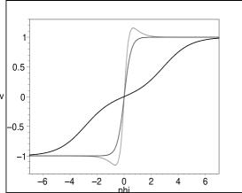
Figure 1: A plot of function $v(\phi)$ for the chosen values of the parameters of the potential $\lambda=1$, $\alpha=10$ – darker curve, $\alpha=1$ – dark-to-gray curve, and $\alpha=0.5$ – soft-gray curve, respectively.

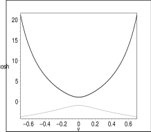
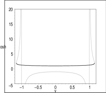
Figure 2: A plot of function $\cosh(\lambda\phi)$ vs $v$, for the chosen values of the free parameters of the potential ($\lambda=1$,$\alpha=10$) – left-hand panel, and ($\lambda=1$,$\alpha=0.5$) – right-hand panel. Both branches of the cosh-function, the positive (dark curve) and the negative one (gray line) are shown. Notice that, for the second case ($\alpha<1$), the whole cosh-function behaviour is depicted by a union of part of the negative and the entire positive branches.

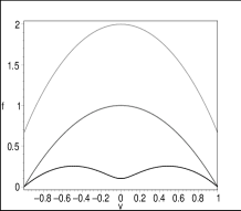
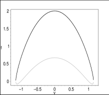
Figure 3: A plot of function $f^{+}$ in Eq.(22) vs $v$, for the chosen values of the free parameters of the potential in Fig.1 – left-hand panel. In the right-hand panel we show a plot of $f$ vs $v$ for $\alpha=0.5<1$ ($\lambda=1$). Both branches of $f(v)$ in Eq.(22), the positive (darker curve) and the negative one (gray line), are depicted.

IV.2 Function $f(v)$ for the cosh-like Potential (5)

We now derive the function $f(v)$ in Eq. (13) (also present in Eq. (14c)), for the potential of interest here (Eq.(5)). According to the definition (11) for the cosh-like potential, one has

$$v(\phi)=\frac{\sinh(\lambda\phi)}{\cosh(\lambda\phi)-1+\alpha}\,,$$ (16)

where $\alpha\equiv\Lambda/V_{0}$. From (16) it follows, in particular, that

$$\lim_{\phi\rightarrow\pm\infty}v(\phi)=\pm 1,\;\lim_{\phi\rightarrow 0}v(\phi)=0\,.$$ (17)

The value $\alpha=1$ is a critical one. Actually, the function (16) is an extremum whenever:

$$\cosh(\lambda\phi)=\frac{1}{1-\alpha},\;\Rightarrow\;v^{2}_{ext}=\frac{1}{\alpha(2-\alpha)}\,.$$ (18)

The fact that the cosh function is always equal or bigger than unity means that $v(\phi)$ is an extremum only if $0<\alpha<1$. For $\alpha\geq 1$ the function $v$ is, at least, a monotonically non-decreasing function as the scalar field takes values in the interval $-\infty<\phi<\infty$, therefore, in this case $v\in[-1,1]$.

In Fig. 1 the function $v(\phi)$ is plotted for the following sets of values of the parameters of the potential $V(\phi)$: ($\lambda=1,\alpha=10$) – dark curve, ($\lambda=1,\alpha=1$) – dark-to-gray curve, and ($\lambda=1,\alpha=0.5$) – soft-gray curve, respectively. As seen, in the latter case, since $\alpha<1$, $v(\phi)$ is a minimum at

$$\lambda\phi=-\text{arc}\cosh(\frac{1}{1-\alpha})=-\text{arc}\cosh(2)\,,$$ (19)

where $v_{min}=-1/\sqrt{\alpha(2-\alpha)}=-\sqrt{4/3}$, while at $\lambda\phi=\text{arc}\cosh(2)$ it is a maximum instead: $v_{max}=\sqrt{4/3}$.

The function $v(\phi)$ in Eq.(16) can be inverted to have the cosh function written in terms of $v$,

$$\cosh(\lambda\phi)^{\pm}(v)=\frac{(\alpha-1)v^{2}\pm\sqrt{1+\alpha(\alpha-2)v^{2}}}{1-v^{2}},$$ (20)

where the ”$\pm$” signs refer to the two different branches of $\cosh(\lambda\phi)(v)$.

For values $\alpha\geq 1$, the mathematical requirement that the cosh-function has to be, neccessarily, bigger than or equal to the unity, leads to the following condition

$$\alpha v^{2}\pm\sqrt{1+\alpha(\alpha-2)v^{2}}\geq 1,\;\Rightarrow\;|v|\leq 1\,,$$ (21)

so that, as already mentioned before, only values of $v$ obeying $|v|\leq 1$ can be considered. This point is relevat when discussing the definition of the phase space since $v$ is one of the variables spanning the phase space of the model under consideration here. For $0<\alpha<1$ the reasoning is not so simple, however, it is clear from the former analysis that, in this case, $|v|\leq|v_{ext}|=1/\sqrt{\alpha(2-\alpha)}$.

In order to illustrate the discussion above, in Fig. 2 we plotted the cosh-function vs $v$ for two sets of values of the parameters of the potential: i) ($\lambda=1,\alpha=10$) – left-hand panel, and ii) ($\lambda=1,\alpha=0.5$) – right-hand panel, respectively. In both cases the darker curve is for the positive branch (”+” sign in Eq. (20)), while the gray line is for the negative branch (”-” sign in Eq. (20)) instead.

Notice from the left-hand panel of Fig. 2 ($\alpha=10>1$), that only the positive branch actually depicts the right (whole) cosh-function behaviour. In the right-hand panel ($\alpha=0.5<1$), instead, the whole cosh-function behaviour can be covered by a union of that part of the negative branch to the left of the vertical asymptote $v=-1$, starting at infinitely large values of $\cosh(\lambda\phi)$ (i. e., infinitely large negative values of $\phi$) until the gray curve meets the dark one (the positive branch) at the union point at $v=v_{min}=-1/\sqrt{\alpha(2-\alpha)}$.

The same is true for positive values of $\phi$: the right cosh-function behaviour is depicted by a union of that part of the negative branch to the right of the vertical asymptote at $v=1$, starting at infinitely large positive values of $\phi$, until it joints the positive branch at $v=v_{max}=1/\sqrt{\alpha(2-\alpha)}$. The range of intermediate-to-small values of $\phi$ (including the beginning at $\phi=0$, where the potential $V(\phi)$ in Eq. (5) is a minimum), is completely covered by the positive branch of the cosh-function (20).

For the potential (5) the function $f(v)$ appearing in Eqs. (13) and (14c), can be written in the following way

$$f^{\pm}(v)=\frac{\pm\left(1-v^{2}\right)\sqrt{1+\alpha(\alpha-2)v^{2}}}{\alpha-1\pm\sqrt{1+\alpha(\alpha-2)v^{2}}}\,,$$ (22)

where the $\pm$ signs refer to the positive and the negative branches of the function $f(v)$ (directly related with the positive and the negative branches of the cosh-function in Eq. (20)), respectively. In Eq. (22) the choice of the ”+” or the ”-” sign is to be made simultaneously in the numerator and in the denominator on the right-hand-side. Hence, for instance, for the positive branch of $f(v)$ one has

$$f^{+}(v)=\frac{+(1-v^{2})\sqrt{...}}{\alpha-1+\sqrt{...}},\;\;\text{etc.}$$ (23)

It has to be emphasized that, while for values of the free parameter $\alpha\geq 1$ the positive branch $f^{+}(v)$ in Eq. (22) is enough to depict the whole dynamics, for $0<\alpha<1$, instead, one needs to contemplate both branches $f^{\pm}(v)$.

Actually, in the later case the piece of the dynamics in the $v$-interval

$$1<|v|\leq\frac{1}{\sqrt{\alpha(2-\alpha)}}\,,$$ (24)

is uncovered by the correponding values of $f^{-}(v)$ in Eq. (22): $f^{-}(|v|>1)$. The rest of the dynamics – including the late-time behaviour – is uncovered by the piece of the positive branch liying in the interval $|v|\leq 1$: $f^{+}(|v|\leq 1)$. In consequence, for $0<\alpha<1$, the whole dynamics is uncovered by

$$f_{0<\alpha<1}=f^{-}(|v|>1)\cup f^{+}(|v|\leq 1)\,.$$ (25)

To summarize, for $\alpha\geq 1$ the cosmic dynamics driven by the potential (5) can be associated with the following 3-dimensional (compact) phase space, spanned by the variables $x$, $y$, and $v$ (we take into account only expanding cosmologies $H\geq 0$)

$$\Psi_{\alpha\geq 1} = \left\{(x,y,v):0\leq x^{2}+y^{2}\leq 1,\right.$$ (26)

$$\;\left.|x|\leq 1,\;0\leq y\leq 1,\;|v|\leq 1\right\},$$

and we have to worry only about the positive branch of $f(v)$ in Eq.(22). Meanwhile, for $0<\alpha<1$, the 3-dimensional (compact) phase space is given by

$$\Psi_{0<\alpha<1} = \left\{(x,y,v):0\leq x^{2}+y^{2}\leq 1,\right.$$ (27)

$$\;\left.|x|\leq 1,\;0\leq y\leq 1,\;|v|\leq\frac{1}{\sqrt{\alpha(2-\alpha)}}\right\},$$

and, depending on the piece of the dynamics one is interested in, one has to rely either on the negative branch of Eq.(22) $f^{-}(|v|>1)$ (early times-to-intermediate dynamics), or on the positive brach instead $f^{+}(|v|\leq 1)$ (late-time dynamics), the whole dynamics being described by $f_{0<\alpha<1}$ in Eq.(25).

In what follows, depending on the value of parameter $\alpha=\Lambda/V_{0}$, we shall look for fixed points of the autonomous system of ODE (14c), with $f(v)$ given, either by: i) the positive branch of equation (22), within the phase space $\Psi_{\alpha\geq 1}$ defined in Eq. (26), whenever $\alpha\geq 1$, or ii) by $f_{0<\alpha<1}$ defined in Eq. (25), within the phase space $\Psi_{0<\alpha<1}$ defined in Eq. (27), if $0<\alpha<1$.

Table 1: Properties of the fixed points for the autonomous system (14c).

$P_{i}$	$x$	$y$	$v$	Existence	$\Omega_{\gamma}$	$\Omega_{\phi}$	$\gamma_{\phi}$	$q$
$P_{1}$	$0$	$0$	$v$	Always	1	$0$	undefined	$-1+\frac{3\gamma}{2}$
$P_{2}$	$1$	$0$	$1$	”	$0$	$1$	$2$	$2$
$P_{3}$	$\frac{\lambda}{\sqrt{6}}$	$\sqrt{1-\frac{\lambda^{2}}{6}}$	$1$	$\lambda\leq\sqrt{6}$	$0$	$1$	$\frac{\lambda^{2}}{3}$	$-1+\frac{\lambda^{2}}{2}$
$P_{4}$	$\sqrt{\frac{3}{2}}\frac{\gamma}{\lambda}$	$\sqrt{\frac{3\gamma(2-\gamma)}{2\lambda^{2}}}$	$1$	$\lambda\geq\sqrt{3\gamma}$	$1-\frac{3\gamma}{\lambda^{2}}$	$\frac{3\gamma}{\lambda^{2}}$	$\gamma$	$-1+\frac{3\gamma}{2}$
$P_{5}$	$0$	$1$	$0$	Always	$0$	$1$	$0$	$-1$

Table 2: Eigenvalues of the linearization matrices corresponding to the fixed points in table 1. We have used the following definition $R\equiv\sqrt{11\gamma^{2}-28\gamma+12\left(1+2\gamma^{2}\left[3\gamma-2+12(1-\gamma)\gamma^{2}/\lambda^{2}-\gamma^{2}(1-3\gamma^{2}/\lambda^{2})\right]/\lambda^{2}\right)}$.

$P_{i}$	$\lambda_{1}$	$\lambda_{2}$	$\lambda_{3}$
$P_{1}$	$-3+3\gamma/2$	$3\gamma/2$	$0$
$P_{2}$	$6-3\gamma$	$3-\sqrt{3/2}\lambda$	$\sqrt{6}\lambda$
$P_{3}$	$-3+\lambda^{2}/2$	$\lambda^{2}-3\gamma$	$\lambda^{2}$
$P_{4}$	$-3(2-\gamma)/4+\sqrt{3}R/4$	$-3(2-\gamma)/4-\sqrt{3}R/4$	$3\gamma$
$P_{5}$	$-3\gamma$	$-3(1-\sqrt{1-4\lambda^{2}/\alpha})/2$	$-3(1+\sqrt{1-4\lambda^{2}/\alpha})/2$

IV.3 Equilibrium Points and Stability

The fixed points of the autonomous system of ODE (14c), in the phase space $\Psi_{\alpha\geq 1}$ defined by Eq. (26) or in $\Psi_{0<\alpha<1}$ defined by Eq. (27), are listed in Table 1, while the eigenvalues of the corresponding linearization matrices are shown in Table 2.

In the case when the parameter $0<\alpha<1$, by looking at the definition of the function $f(v)$ in Eq. (22), it might seem that, in addition to the critical points in Table 1, there can be also equilibrium points associated with the values $v=\pm 1/\sqrt{\alpha(2-\alpha)}$. However, if one looks at Fig. 3 (right-hand panel), one can see that at $v=\pm 1/\sqrt{\alpha(2-\alpha)}$ the derivative of the function $f_{0<\alpha<1}$ in Eq. (25), is undefined, so that the linear approach undertaken in this investigation is not valid any more. This means that the above points in phase space might not be actual critical points, so that we shall not include them in our analysis.

Existence of the matter-dominated solution (equilibrium point $P_{1}$ in Table 1), is independent on the value of the variable $v$, meaning that this phase of the cosmic evolution may arise at early-to-intermediate times, as well as at late times. As seen from Table 2, since in this case the two non vanishing eigenvalues of the linearization matrix are of oposite sign, the matter-dominated solution is always a saddle equilibrium point of Eqs. (14c).

Equilibrium points $P_{2}$, $P_{3}$, and $P_{4}$, are associated with early time dynamics since, according to Eq. (16), $v=1$ is correlated with infinitely large values of the variable $\phi$. Besides, in this case,

$$\partial_{\phi}\ln V=-\lambda,\;\Rightarrow\;V=\bar{V}_{0}e^{-\lambda\phi}\,$$ (28)

in correspondence with the limit of potential (5) at large $\phi$’s. This confirms that equilibrium points with $v=1$, indeed correspond to early-times dynamics in the model with the cosh-like potential (5). The main porperties of these equilibrium points ($P_{2}-P_{4}$), together with those of the matter-dominated phase $P_{1}$, have been discussed inwands . These can be summarised as follows (the properties of the matter-dominated solution $P_{1}$ have been discussed above):

• The kinetic energy-dominated solution (point $P_{2}$ in Table 1), is always decelerating. For $\lambda\leq\sqrt{6}$ it is the past attractor for any phase space trajectory.

• The scalar field-dominated solution (equilibrium point $P_{3}$), exist whenever $\lambda\leq\sqrt{6}$, and it is inflacionary for $\lambda<\sqrt{2}$ (decelerating otherwise). It is always a saddle point in the phase space $\Psi$ defined in Eq. (26).

• The scaling solution (fixed point $P_{4}$), exists whenever $\lambda\geq\sqrt{3\gamma}$. This solution is correlated with decelerated expansion of the universe for $\gamma\geq 2/3$ (it is inflationary otherwise). The $\phi$-field mimics matter with a barotropic index $\gamma_{\phi}=\gamma$, while their energy densities scale as

  $$\frac{\Omega_{\phi}}{\Omega_{\gamma}}=\frac{1}{\lambda^{2}/3\gamma-1}\,.$$ (29)

  It is always a saddle point in $\Psi$.

• The late-time dynamics driven by potential (5) is correlated with the minimum $V_{min}=\Lambda$ at $\phi=0$ – and its neigbourhood –, which, in the phase space $\Psi$, is depicted by the equilibrium point with $v=0$ in Table 1 (point $P_{5}$). This point corresponds to the inflationary de Sitter solution $3H^{2}=\Lambda$. Since the real parts of the eigenvalues of the linearization matrix for $P_{5}$ are all negative (see Table 2), the de Sitter solution is always the future attractor for any phase space trajectory.

For values of the parameter $\lambda>\sqrt{\alpha}/2$, the de Sitter attractor is a spiral fixed point and, whenever $\alpha<24$ both, the past attractor (point $P_{2}$), and the future (late-time) attractor (point $P_{5}$) co-exist, meaning that the corresponding orbits in the phase space will be repelled by the kinetic energy-dominated solution and will be eventually attracted to the de Sitter solution.

In this case ($\lambda>\sqrt{\alpha}/2$), the linear perturbations of the scalar field perform damped oscillations around the minimum of the potential at $\phi=0\;\Rightarrow\;v=0$, that are characterized by cyclic frequency

$$\omega=\frac{3}{2}\sqrt{\frac{4\lambda^{2}}{\alpha}-1}\,.$$ (30)

For $\lambda^{2}>\alpha/4$, the general solution for the evolution of linear perturbations $\delta x_{i}=(\delta x,\delta y,\delta v)$ in the neighbourhood of the minimum of the potential (equilibrium point $P_{5}$ in tables Tables 1 and 2), can be written as

$$\delta x_{i} = a_{i1}e^{\lambda_{1}\tau}+a_{i2}e^{\lambda_{2}\tau}+a_{i3}e^{\lambda_{3}\tau}$$ (31)

$$= a_{i1}e^{-3\gamma\tau}+e^{-3\tau/2}\left(a_{i2}\,e^{i\omega\tau}+a_{i3}\,e^{-i\omega\tau}\right)\,,$$

where $\lambda_{1}$, $\lambda_{2}$, and $\lambda_{3}$ are the eigenvalues of the linearization matrix around $P_{5}$.

The latter oscillatory behaviour with frequency $\omega$ is what, according to Refs.wang ; further ; mul , can be associated with cold dark matter because the amplitudes of the perturbations decrease at a rate $\propto\exp{(-3\tau/2)}$. The corresponding mean energy density $\left\langle\rho_{\phi}\right\rangle$ then dilutes at a rate $\propto a^{-3}$ with an effective equation of state $\left\langle\omega_{\phi}\right\rangle=0$ (see Eq. (2)).

The above results are illustrated in Fig. 4 and Fig. 5 for a fixed value $\gamma=4/3$. In particular, the oscillating solution is depicted in the latter figure, where it is apparent the way the orbits of the ODE (14c), at late times, coil around the segment $\{(x,y,v)=(0,y,0):0\leq y\leq 1\}$ until, eventually they reach the inflationary de Sitter attractor $P_{5}=(0,1,0)$. The oscillating solution arises due to the choice of the free parameters in Fig. 5: $\lambda=5,\;\alpha=3$, that obey the constraint $\lambda>\sqrt{\alpha}/2$.

For self-consistency, we show in Figs. 6 and 7 the late-time (point $P_{5}$ above, associated with the neighbourhood of the minimum of the potential), and early-to-intermediate times local behaviours of the orbits of Eqs. (14c), respectively, for small values of the parameter $\alpha$ ($0<\alpha<1$).

Due to the choice of the values of the free parameters ($\lambda=2,\alpha=0.1$), obeying $\lambda^{2}>\alpha/4$ as in the former case, since the corresponding equilibrium point is a spiral one, the orbits coil around the de Sitter segment $(x,y,v)=(0,y,0)$ until, eventually, they reach the de Sitter solution $3H=\Lambda$ (Fig. 6). The early times-to-intermediate behaviour (Fig. 7), clearly shows that the kinet energy-dominated solution (equilibrium point $P_{2}$) is the past attractor, while the matter-scaling solution (point $P_{4}$) is a saddle equilibrium point.

We want to emphasize that the above spiral form of the orbits of the ODE (14c) – see Fig. 6 – is what can be properly correlated with CDM behavior, so that, only for $\lambda>\sqrt{\alpha}/2$ the scalar field component in our model may be called as SFDM.

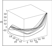
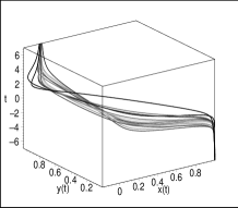
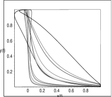
Figure 4: Orbits of the autonomous system of ODE (14c) with function $f(v)$ in Eq. (22), and the corresponding flux in time $\tau$ – upper panels –, for the chosen values of the parameters ($\lambda=2$, $\alpha=10$, $\gamma=4/3$– background radiation), for different sets of initial conditions. In the lower panel we show the projection of the orbits into the phase plane $(x,y)$. Notice that the kinetic energy-dominated solution $(x,y,v)=(1,0,1)$ is the past attractor, while the de Sitter solution $(0,1,0)$ is the future attractor. The radiation-dominated solution $(0,0,v)$ is always a saddle fixed point for any given $v$.

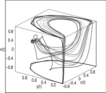
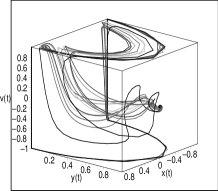
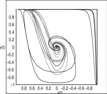
Figure 5: Different perspectives of the local late-time behaviour of the orbits of the autonomous system of ODE (14c), with function $f(v)$ in Eq. (22), for different values of the parameters $\lambda=5$, and $\alpha=3$ ($\gamma=4/3$– background radiation) – upper panels. In the lower panel we show the projection of the orbits into the phase plane $(x,v)$. At late times the phase space trajectories coil around the de Sitter segment $\{(0,y,0):0\leq y\leq 1\}$ until, eventually, they reach the inflationary de Sitter attractor $(0,1,0)$.

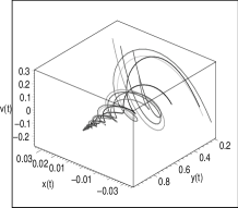
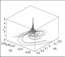
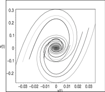
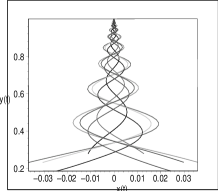
Figure 6: Local behaviour of the orbits of the autonomous system of ODE (14c) with function $f(v)$ in Eq. (25), in the neightbourhood of the point $P_{5}$ associated with late-time cosmic dynamics, and the corresponding flux in time $\tau$ – upper panels –, for the chosen values of the parameters: $\lambda=2$, $\alpha=0.1$ ($\gamma=4/3$– background radiation), for different sets of initial conditions. In the lower panel we show the projection of the orbits into the phase planes $(x,v)$ and $(x,v)$, respectively.

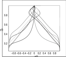
Figure 7: Early times-to-intermediate behaviour of the orbits of the autonomous system of ODE (14c) with function $f(v)$ in Eq. (25), for the chosen values of the parameters: $\lambda=2$, $\alpha=0.1$ ($\gamma=4/3$– background radiation), for different sets of initial conditions. In the right-hand panel we show the projection of the orbits into the phase plane $(x,v)$. It is evident that the kinetic energy-dominated solution (point $P_{2}$ in Tab.1) is the past attractor, while the scaling solution (point $P_{4}=(0.81,0.71,1)$) is a saddle equilibrium point.

V Summary of Results

The relevant results of the study of the fixed points of the autonomous system of ODE (14c), for the cosh-like potential $V(\phi)$ in Eq. (5) – corresponding to $f(v)$ in Eq. (22) –, can be summarized as follows (see the former section).

• The past (early-time) attractor in the phase space $\Psi$, for $\lambda<6$, is the kinetic energy-dominated (decelerated) solution $3H^{2}=\dot{\phi}^{2}/2$ (see Fig.4). For values $\lambda\geq 6$ there does not exist any past attractor in $\Psi$ (see Fig.5).

• The scalar field-dominated phase $3H^{2}=\dot{\phi}^{2}/2+V(\phi)$ (existing only for $\lambda^{2}\leq 6$, and inflationary whenever $\lambda<\sqrt{2}$), and the scaling solution $\Omega_{\phi}/\Omega_{\gamma}=1/[(\lambda^{2}/3\gamma)-1]$ (exists whenever $\lambda^{2}\geq 3\gamma$, decelerating if $\gamma\geq 2/3$), are always saddle equilibrium points.

• The (decelerating) matter-dominated solution $3H^{2}=\rho_{\gamma}$ exists for any value $v$ in $\Psi$. It always represents a saddle fixed point (see Fig. 4).

• The future attractor is always the inflationary de Sitter solution $3H^{2}=\Lambda$. At late times, for $\lambda>\sqrt{\alpha}/2$, the orbits of the ODE (14c) coil around the de Sitter segment $\{(0,y,0):0\leq y\leq 1\}$ until, eventually, these reach the late-time de Sitter attractor $3H^{2}=\Lambda$ (see Fig. 5). The later (late-time) behaviour can be associated with oscillating solutions that reproduce CDM in the model.

In the next section we will discuss the relevance of the above results to the cosmology of the model under investigation.

VI Discussion and Conclusions

The fact that the scaling solution (point $P_{4}$ in Table 1), the matter-dominated phase (point $P_{1}$), and the de Sitter inflationary solution ($P_{5}$) are equilibrium points of Eqs. (14c) for the potential (5), is not a happy coincidence but a profound principle of nature, inherent in the SFDM model with cosh-like potential under investigation in this paper.

In terms of the dynamical systems analysis this means, in particular, that independent on the initial conditions chosen, there is a chance for the cosmological model to transit by each of the mentioned phases, spending some time in the neighbourhood of each one of them. More precisely, independent on the initial conditions, the cosmological evolution might drive the universe from one phase to another to, inevitably, end up in the de Sitter stage (point $P_{5}$) being the late-time attractor in the phase space of the model ($\Psi$).

The cosmic evolution driven by the $\phi$-field after the end of inflation, most probably starts in the neightbourhood of $P_{4}$ where the scalar field tracks matter (radiation). Then, at early-to-intermediate times it approaches to the matter-dominated (decelerated) stage $P_{1}$ where most structure was formed until, finally, the evolution end ups in the inflationary de Sitter stage $P_{5}$.

The fact that, for appropriate values of the free parameters ($\lambda>\sqrt{\alpha}/2$), the latter solution is a spiral equilibrium point means that, at late times, while the phase space trajectories approach to the de Sitter phase, the scalar field perturbations perform damped oscillations that mimic CDM. Therefore the SFDM model with a cosh-like potential could also be a nice scenario to address the united description of the dark matter and of the dark energy in a single fieldcul .

- (1) L. Bergstrom, arXiv:0903.4849 [hep-ph].
- (2) M. Srednicki, Eur.Phys.J.C15:143-144,2000.
- (3) A. Del Popolo, arXiv:0801.1091 [astro-ph].
- (4) D. Samtleben, S. Staggs and B. Winstein, Ann. Rev. Nucl. Part. Sci. 57, 245 (2007) [arXiv:0803.0834 [astro-ph]].
- (5) A. Burkert, IAU Symp. 171, 175 (1996) [Astrophys. J. 447, L25 (1995)] [arXiv:astro-ph/9504041].
- (6) B. Moore, Nature 370, 629 (1994). W. J. G. de Blok, S. S. McGaugh, A. Bosma and V. C. Rubin, Astrophys. J. 552, L23 (2001) [arXiv:astro-ph/0103102].
- (7) J. A. Tyson, G. P. Kochanski and I. P. Dell’Antonio, Astrophys. J. 498, L107 (1998) [arXiv:astro-ph/9801193].
- (8) T. Matos and F. S. Guzman, Class. Quant. Grav. 17, L9 (2000) [arXiv:gr-qc/9810028].
- (9) E. J. Copeland, M. Sami and S. Tsujikawa, Int. J. Mod. Phys. D15 (2006) 1753-1936 [hep-th/0603057].
- (10) A. Bernal, T. Matos and D. Nunez, Rev. Mex. A.A. 44, (2008), 149-160 [arXiv:astro-ph/0303455].
- (11) T. Matos and L. A. Urena-Lopez, Phys. Rev. D 63, 063506 (2001) [arXiv:astro-ph/0006024].
- (12) T. Matos and L. A. Urena-Lopez, Class. Quant. Grav. 17, L75 (2000) [arXiv:astro-ph/0004332].
- (13) V. Sahni and L. M. Wang, Phys. Rev. D 62, 103517 (2000) [arXiv:astro-ph/9910097].
- (14) T. Matos, J. A. Vazquez and J. Magana, arXiv:0806.0683 [astro-ph].
- (15) V. A. Belinsky, I. M. Khalatnikov, L. P. Grishchuk and Y. B. Zeldovich, Phys. Lett. B 155, 232 (1985). A. de la Macorra and G. Piccinelli, Phys. Rev. D 61, 123503 (2000) [arXiv:hep-ph/9909459]. L. A. Urena-Lopez and M. J. Reyes-Ibarra, arXiv:0709.3996 [astro-ph].
- (16) M. S. Turner, Phys. Rev. D 28, 1243 (1983).
- (17) A. A. Coley, Dordrecht, Netherlands: Kluwer (2003) 200 p. A. A. Coley, arXiv:gr-qc/9910074.
- (18) E. J. Copeland, A. R. Liddle and D. Wands, Phys. Rev. D 57, 4686 (1998) [arXiv:gr-qc/9711068].
- (19) W. Fang, Y. Li, K. Zhang and H. Q. Lu, arXiv:0810.4193 [hep-th].
- (20) A. R. Liddle and L. A. Urena-Lopez, Phys. Rev. Lett. 97, 161301 (2006) [arXiv:astro-ph/0605205]. A. R. Liddle, C. Pahud and L. A. Urena-Lopez, Phys. Rev. D 77, 121301 (2008) [arXiv:0804.0869 [astro-ph]].