Abstract

The BPS equations in M-theory for solutions with 16 residual supersymmetries, $SO(2,2)\times SO(4)\times SO(4)$ symmetry, and $AdS_{4}\times S^{7}$ asymptotics, were reduced in [arXiv:0806.0605] to a linear first order partial differential equation on a Riemann surface with boundary, subject to a non-trivial quadratic constraint. In the present paper, suitable regularity and boundary conditions are imposed for the existence of global solutions. We seek regular solutions with multiple distinct asymptotic $AdS_{4}\times S^{7}$ regions, but find that, remarkably, such solutions invariably reduce to multiple covers of the M-Janus solution found by the authors in [arXiv:0904.3313], suggesting rigidity of the half-BPS M-Janus solution. In particular, we prove analytically that no other smooth deformations away from the M-Janus solution exist, as such deformations invariably violate the quadratic constraint. These rigidity results are contrasted to the existence of half-BPS solutions with non-trivial 4-form fluxes and charges asymptotic to $AdS_{7}\times S^{4}$. The results are related to the possibility of M2-branes to end on M5-branes, but the impossibility of M5-branes to end on M2-branes, and to the non-existence of half-BPS solutions with simultaneous $AdS_{4}\times S^{7}$ and $AdS_{7}\times S^{4}$ asymptotic regions.

1 Introduction

One of the most important realizations of the AdS/CFT correspondence [2, 3, 4] (for reviews, see [5, 6]) in M-theory is the duality of the $AdS_{4}\times S^{7}$ vacuum and the 3-dimensional CFT which is obtained by a decoupling limit of the M2-brane world-volume theory [7, 8]. This 3-dimensional CFT, as well as its dual $AdS_{4}\times S^{7}$ supergravity solution, preserve the maximal number of 32 supersymmetries, and exhibit $SO(2,3)\times SO(8)$ global symmetry. While the M2-brane world-volume CFT is still not completely understood, significant progress has been made over the past few years in constructing a Lagrangian realization in which all or most of the symmetries and supersymmetries are realized explicitly [9, 10, 11, 12].

The insertion of local and/or non-local gauge-invariant operators in the CFT will break some or all of the supersymmetries and global symmetries, and lead to supergravity duals with correspondingly reduced symmetries. An exciting theoretical laboratory is provided by supergravity solutions with 16 residual supersymmetries (or half-BPS solutions). A general classification via semi-simple Lie superalgebras was given in [13] for half-BPS solutions in M-theory which are locally asymptotic to $AdS_{4}\times S^{7}$. An analogous classification for solutions locally asymptotic to $AdS_{7}\times S^{4}$ in M-theory, and locally asymptotic to $AdS_{5}\times S^{5}$ in Type IIB were also obtained there. These supergravity solutions form families in which the corresponding space-time exhibits a warped $AdS$-factor, and they are dual to scale-invariant quantum field theories. Remarkably, the corresponding half-BPS equations may often be reduced to integrable systems, which may then be solved completely, and exactly. The solutions exhibit a wealth of topological and metrical structure, and are characterized by interesting, and generally complicated, moduli spaces.

It was shown in [14] that all solutions to M-theory which are half-BPS, exhibit global $SO(2,2)\times SO(4)\times SO(4)$ symmetry, and are locally asymptotic to either $AdS_{4}\times S^{7}$ or to $AdS_{7}\times S^{4}$, may be constructed via a warped product $AdS_{3}\times S^{3}\times S^{3}$ over a 2-dimensional Riemann surface $\Sigma$, and a certain integrable system on $\Sigma$. Physically, these solutions will be relevant as AdS/CFT duals to CFTs with various arrangements of defects and/or interfaces. The solutions of [14] are local supergravity solutions in the sense that the associated bosonic supergravity fields satisfy the Bianchi and field equations locally, and the corresponding BPS equations allow for 16 independent spinor solutions, locally. The local solutions may or may not be globally regular or physical (e.g. the metric may fail to be real throughout).

To obtain regular physically acceptable solutions (such as those allowed to enter the AdS/CFT correspondence), one must impose global regularity and boundary conditions. For the half-BPS solutions locally asymptotic to $AdS_{7}\times S^{4}$ (which were referred to as cases II and III in [14]), suitable global regularity and boundary conditions were obtained in [22], and the resulting globally regular solutions were constructed using a simple linear superposition principle. Each solution is invariant under the superalgebra $OSp(4^{*}|2)\oplus OSp(4^{*}|2)$. The resulting families of solutions are labelled by an integer $g\geq 0$, and the solutions within each family are described by $2g+1$ independent real moduli. These solutions are fully back-reacted supergravity solutions dual to the supersymmetric self-dual string solution of the 6-dimensional $(2,0)$ super-symmetric M5-brane world-volume theory.

The purpose of the present paper is to impose suitable regularity and boundary conditions on the local half-BPS solutions of [14] which are locally asymptotic to $AdS_{4}\times S^{7}$ (referred to as case I there), and to investigate their existence. Solutions of this type are invariant under the superalgebra $OSp(4|2,{\bf R})\oplus OSp(4|2,{\bf R})$. One new class of such solutions was obtained in [23], and referred to as the M-Janus solution. It consists of a 1-parameter family of deformations of $AdS_{4}\times S^{7}$ which give a holographic realization of a Janus-like defect/interface CFT. The existence of Janus-like solutions in M-theory is surprising, as M-theory contains no dilaton field. Still, in [23], these solutions were obtained analytically, and were found to be regular. Thus, the goal of this paper reduces to investigating the existence of deformations of $AdS_{4}\times S^{7}$ beyond those of the M-Janus solution.

The regularity and boundary conditions for half-BPS solutions locally asymptotic to either $AdS_{4}\times S^{7}$ or $AdS_{7}\times S^{7}$ are as follows. Locally, all such solutions may be constructed in terms of a real, positive harmonic function $h$ on a Riemann surface $\Sigma$, and a complex-valued function $G$ on $\Sigma$ which satisfies a first order partial differential equation [14],

$$\partial_{w}G={1\over 2}(G+\bar{G})\,\partial_{w}\ln h$$ (1.1)

for an arbitrary local complex coordinate system $w,\bar{w}$ on $\Sigma$. This partial differential equation, which is common to all cases I, II, and III, is to be supplemented with a non-linear algebraic constraint, and with boundary conditions which are case-dependent [14]. These conditions are as follows,

Asymptotic to $AdS_{4}\times S^{7}$

(case I)

• local regularity condition: $|G|^{2}>1$ inside $\Sigma$;

• boundary conditions: $h=0$, and $G=+i$ or $G=-i$ on $\partial\Sigma$.

Asymptotic to $AdS_{7}\times S^{4}$

(cases II and III)

• local regularity condition: $-4|G|^{4}-(G-\bar{G})^{2}>0$ inside $\Sigma$;

• boundary conditions: $h=0$, and $G=0$ or $G=i$ on $\partial\Sigma$.

For fixed $h$, the partial differential equation (4.17) is linear in $G$ (under linear superpositions of $G$ with real coefficients). Locally on $\Sigma$, a complex coordinate system may be chosen for which $h={\rm Im}(w)$. The differential equation (4.17) is then invariant under translations of ${\rm Re}(w)$, and may be solved in terms of Fourier transforms of combinations of modified Bessel functions [14]. Even locally, however, the algebraic constraints on $G$ still need to be point-wise enforced, making the problem effectively non-linear.

In the case of solutions which are locally asymptotic to $AdS_{7}\times S^{4}$, nonetheless, the harmonic function $h$ could be used as a global coordinate. Physically, this was possible because the supergravity solutions have only a single $AdS_{7}\times S^{4}$ asymptotic region. The function $G$ could be obtained by a simple linear superposition and, remarkably, the algebraic constraints turned out to be automatically obeyed [22].

In the case of solutions which are locally asymptotic to $AdS_{4}\times S^{7}$, however, the boundary conditions listed above require the space-time to contain multiple asymptotic $AdS_{4}\times S^{7}$ regions. In this case, $h$ is generally not a good global coordinate. Therefore, the Riemann surface $\Sigma$, the harmonic function $h$, and the function $G$, must all be considered as unknowns. This situation renders the system for solutions asymptotic to $AdS_{4}\times S^{7}$ “more non-linear” than the one for the $AdS_{7}\times S^{4}$ case, thus more complicated, with physically different results.

Surprisingly, we find that for locally asymptotic $AdS_{4}\times S^{7}$ boundary conditions, the only regular deformations of the M-Janus solutions are of a topological nature, and produce multiple covers of the basic M-Janus solution. In particular, we shall show analytically that no non-trivial continuous infinitesimal deformations exist away from the M-Janus solution, and give numerical evidence that no finite deformations exist either. These arguments are presented within the context of a set of mild assumptions on the structure of the general regular solutions, which we regard as natural. However, the possibility of solutions containing a localized singularity corresponding to the insertion of a singular M5-brane into $AdS_{4}\times S^{7}$ is still an open problem.

The absence, on the AdS side, of regular half-BPS deformations away from the M-Janus solution has a surprising consequence on the dual CFT side. It implies the non-existence of half-BPS interface/defect operators, in the dual $2+1$-dimensional maximally supersymmetric CFT, which would correspond to such deformations. In ABJM theory, 24 supersymmetries are manifest on the local fields of the QFT for all values of $k$, and one would expect many interface/defect operators which preserve 12 supersymmetries. The remaining 8 supersymmetries of the theory for $k=1,2$ are not manifest but emerge from non-local “monopole operators”, or more accurately from instantons in $2+1$dimensions. Enhancing the 12 supersymmetries of any interface/defect operator to 16 should probably again be caused by instantons, but their geometry may or may not be consistent with the presence of an interface. The results of the current paper suggest that such enhancements to interface/defect operators with 16 supersymmetries should not exist. We plan to investigate these CFT questions in future work.

Throughout the course of our investigations into the existence of solutions to the differential equation (4.17), we provide various reformulations of the problem, which may be of interest in their own right. First, we show that equation (4.17) is equivalent to an $SL(2,{\bf R})$-invariant Helmholtz-like, or automorphic, equation. Second, we show that the general solution of the differential equation (4.17), and its related automorphic equation, may be reformulated in terms of the Hermitian pairing of a number of meromorphic functions (or meromorphic blocks) on $\Sigma$. Third, we show that the general solution to the differential and algebraic constraint equations for solutions asymptotic to $AdS_{7}\times S^{4}$ (obtained in [22]) are given by the Helgason transform corresponding to a certain non-unitary representation of $SL(2,{\bf R})$. Finally, we show that the solutions to the differential equation (4.17) for the case asymptotic to $AdS_{4}\times S^{7}$ also correspond to a non-unitary representation of $SL(2,{\bf R})$, but whose role in mathematics appears to be, thus far, unclear. Similarly, the role in $SL(2,{\bf R})$-representation theory of the non-linear constraints remains to be elucidated.

The structure of the remainder of this paper is as follows. In section 2, we shall review the local solution, the regularity and the boundary conditions for solutions which are locally asymptotic to $AdS_{4}\times S^{7}$. In section 3, we shall review the M-Janus solutions, and construct their multiple covers. In section 4, we shall show that the general local solution may be expressed in terms of Hermitian pairings of certain meromorphic functions, and discuss the $SL(2,{\bf R})$ group theoretic underpinnings of the $AdS_{4}\times S^{7}$ as well as of the $AdS_{7}\times S^{4}$ solutions. In section 5, we shall show that the general natural Hermitian pairing structure for $AdS_{4}\times S^{7}$ always leads to configurations that violate the quadratic constraint $|G|^{2}>1$. In section 6, we shall interpret our rigidity results in terms of the dynamics of M2- and M5-branes. Finally, in section 7, we shall conclude with a discussion of loose ends, open problems and questions for future investigations. Two technical discussions are relegated to Appendices A and B.

2 Local solution, regularity, and boundary conditions

In this section, we review the local half-BPS solutions obtained in [14]. (Derivations may be found in [14]; they will not be needed here, and will not be repeated.) The 11-dimensional metric Ansatz consists of a fibration of $AdS_{3}\times S^{3}\times S^{3}$ over a 2-dimensional Riemann surface $\Sigma$ with boundary $\partial\Sigma$,

$$ds^{2}=f_{1}^{2}ds_{AdS_{3}}^{2}+f_{2}^{2}ds_{S_{2}^{3}}^{2}+f_{3}^{2}ds_{S_{3}^{3}}^{2}+ds_{\Sigma}^{2}$$ (2.1)

The 4-form field strength is given by

$$F_{4}=g_{1a}\;\omega_{AdS_{3}}\wedge e^{a}+g_{2a}\;\omega_{S_{2}^{3}}\wedge e^{a}+g_{3a}\;\omega_{S_{3}^{3}}\wedge e^{a}$$ (2.2)

where $\omega_{AdS_{3}}$ and $\omega_{S^{3}_{2,3}}$ are the volume forms on $AdS_{3}$ and $S^{3}_{2,3}$ respectively, and $e^{a},a=1,2$ is an orthonormal frame on $\Sigma$. In terms of an arbitrary system of local complex coordinates $w,\bar{w}$ on $\Sigma$, the metric on $\Sigma$ in (2.1) reduces to the standard conformal form,

$$ds_{\Sigma}^{2}=4\rho^{2}|dw|^{2}$$ (2.3)

The metric factors $f_{1},f_{2},f_{3},\rho$, as well as the flux fields $g_{1a},g_{2a}$, and $g_{3a}$, only depend on $\Sigma$. The Ansatz automatically respects $SO(2,2)\times SO(4)\times SO(4)$ symmetry, which may also be viewed as the symmetry of an AdS/CFT dual 1+1-dimensional conformal interface or defect in the 3-dimensional M2-brane CFT.

In [14], the BPS equations governing solutions with 16 residual supersymmetries were reduced to constructing a Riemann surface $\Sigma$ with boundary, a real positive harmonic function $h$ on $\Sigma$, and the solution to a first order partial differential equation on $\Sigma$ for a complex-valued field $G$, subject to a point-wise non-linear algebraic constraint. (The origin of $G$ in terms of Killing spinor components, and its relations to these spinors may be found in [14].) The partial differential equation for $G$ is given by,

$$2\partial_{w}G=(G+\bar{G})\partial_{w}\ln h$$ (2.4)

for an arbitrary complex coordinate system $w,{\bar{w}}$ on $\Sigma$. For solutions locally asymptotic to $AdS_{4}\times S^{7}$ (case I), the field $G$ is subject to the following point-wise quadratic constraint,

$$|G(w,{\bar{w}})|^{2}>1\qquad{\rm for~{}all}\qquad(w,{\bar{w}})~{}\hbox{on the inside of}~{}\Sigma$$ (2.5)

For any given harmonic function $h$, the differential equation (2.4) is linear in the sense that if $G_{1}$ and $G_{2}$ are two solutions of (2.4), then so is $\lambda_{1}G_{1}+\lambda_{2}G_{2}$, where $\lambda_{1},\lambda_{2}$ are real constants. Since the complex coordinates $w,\bar{w}$ are arbitrary, we may choose locally ${\rm Im}(w)=h$, and then solve the equation (2.4) by Fourier analysis, as was done in [14]. To solve the full set of reduced BPS equations, however, it remains to enforce the point-wise quadratic constraint (2.5), which poses a highly non-trivial problem.

2.1 The real field $\Phi$

In all generality, the equation (2.4) for $G$ may be partially integrated in terms of a single real function. To see this, we multiply (2.4) on both sides by the anti-holomorphic 1-form $\partial_{\bar{w}}h$. This gives the following equation,

$$\partial_{w}\left(G\partial_{\bar{w}}h\right)=(G+\bar{G}){|\partial_{w}h|^{2}\over 2h}$$ (2.6)

Since the right hand side of this equation is real, we have $\partial_{w}\left(G\partial_{\bar{w}}h\right)=\partial_{\bar{w}}\left(\bar{G}\partial_{w}h\right)$. As a result there exists, at least locally, a real function $\Phi$ such that $G(\partial_{\bar{w}}h)=\partial_{\bar{w}}\Phi$. Actually, the Riemann surfaces of interest to us here will always be contractible, and $\Phi$ will be singularity-free on the inside of $\Sigma$, so that the local result will hold globally on $\Sigma$. Thus, $\Phi$ provides a partial integral of (2.4), as well as an economical parameterization of $G$, given by,

$$G={\partial_{\bar{w}}\Phi\over\partial_{\bar{w}}h}$$ (2.7)

Equation (2.4) expressed in terms of $\Phi$ takes the form,

$$2\partial_{w}\partial_{\bar{w}}\Phi-\partial_{\bar{w}}\Phi(\partial_{w}\ln h)-\partial_{w}\Phi(\partial_{\bar{w}}\ln h)=0$$ (2.8)

In terms of the field $\Phi$, the quadratic constraint (2.5) becomes an inequality on the derivatives of $\Phi$, given by $|\partial_{w}\Phi|^{2}\geq|\partial_{w}h|^{2}$.

2.2 Metric factors and anti-symmetric tensor in terms of $G$ and $h$

In order to express in terms of $h$ and $G$ the local half-BPS solutions which are locally asymptotic to $AdS_{4}\times S^{7}$, and investigate their regularity and boundary conditions, it will be useful to define the following real function $W^{2}$ on $\Sigma$,

$$W^{2}\equiv 4|G|^{4}+(G-\bar{G})^{2}$$ (2.9)

Assuming that $|G|^{2}\geq 1$, we automatically have $W^{2}\geq 0$. The metric factors in (2.1) are then expressed as follows,

$$f_{1}^{6} = {h^{2}W^{2}\over 16^{2}(|G|^{2}-1)^{2}}$$

$$f_{2}^{6} = h^{2}{(|G|^{2}-1)\over 4\,W^{4}}\left(2|G|^{2}+i(G-\bar{G})\right)^{3}$$

$$f_{3}^{6} = h^{2}{(|G|^{2}-1)\over 4\,W^{4}}\left(2|G|^{2}-i(G-\bar{G})\right)^{3}$$ (2.10)

The metric factor in (2.3) is given by,

$$\rho^{6} = {\left|\partial_{w}h\right|^{6}\over 16^{2}h^{4}}\big{(}|G|^{2}-1\big{)}W^{2}$$ (2.11)

The anti-symmetric tensor field-strengths are expressed in terms of $g_{i}$. They can be defined by conserved currents as follows,

$$(f_{1})^{3}g_{1w}=-\partial_{w}b_{1} = {3W^{2}\partial_{w}h\over 32G(|G|^{2}-1)}-{1+G^{2}\over 16G(|G|^{2}-1)^{2}}\,J_{w}$$

$$(f_{2})^{3}g_{2w}=-\partial_{w}b_{2} = -{(G+i)(2|G|^{2}+i(G-\bar{G}))^{2}\over W^{4}}\,J_{w}$$

$$(f_{3})^{3}g_{3w}=-\partial_{w}b_{3} = +{(G-i)(2|G|^{2}-i(G-\bar{G}))^{2}\over W^{4}}\,J_{w}$$ (2.12)

where the following quantity was used for notational compactness,

$$J_{w}={1\over 2}(G\bar{G}-3\bar{G}^{2}+4G\bar{G}^{3})\partial_{w}h+hG\partial_{w}\bar{G}$$ (2.13)

It was shown in [14] that the equations of motion of as well as the Bianchi identities are satisfied for a harmonic $h$ and a $G$ which solves (2.4).

2.3 The $AdS_{4}\times S^{7}$ solution

The simplest solution is the maximally symmetric $AdS_{4}\times S^{7}$ itself. The Riemann surface is the infinite strip,

$$\Sigma=\{w\in{\bf C},~{}w=x+iy,~{}x\in{\bf R},\;0\leq y\leq\pi/2\}$$ (2.14)

Note that the Riemann surface $\Sigma$ has two boundary components. In these coordinates, the functions $h$ and $G$ for the $AdS_{4}\times S^{7}$ solution are given by,

$$G=i{{\rm\,ch}(w+\bar{w})\over{\rm\,ch}(2\bar{w})} \left\{\matrix{h=8\,{\rm Im}({\rm\,sh}(2w))\cr\Phi=-8{\rm\,sh}(w+\bar{w})\cr}\right.$$ (2.15)

Using (2.2), the metric factors become,

$$f_{1}={\rm\,ch}(2x)\qquad f_{2}=-2\cos(y)\qquad f_{3}=-2\sin(y)\qquad\qquad\rho=1$$ (2.16)

The boundary is characterized by the vanishing of the harmonic function $h=0$, or alternatively, by $G=\pm i$. On the lower boundary of the strip, where $y=0$, one has $G=+i$, which implies that the radius $f_{2}$ of $S_{2}^{3}$ vanishes. On the upper boundary of the strip, where $y=\pi/2$, one has $G=-i$, which implies that the radius $f_{3}$ of $S_{3}^{3}$ vanishes. The boundary of $AdS_{4}\times S^{7}$ on the other hand is located at $x=\pm\infty$. An additional piece of the $AdS_{4}\times S^{7}$ boundary is located at the $1+1$-dimensional boundary of the $AdS_{3}$ fiber, along which the $x=+\infty$ and $x=-\infty$ pieces of the boundary are glued together.

2.4 General Regularity and boundary conditions

Physically interesting solutions generally require solutions to be everywhere regular and to be locally asymptotic to $AdS_{4}\times S^{7}$. This leads to the following three assumptions for the geometry of each solution.

1. The boundary of the 11-dimensional geometry is locally asymptotic to $AdS_{4}\times S^{7}$.

2. The metric factors are finite everywhere on $\Sigma$, except at points where the geometry becomes locally asymptotic to $AdS_{4}\times S^{7}$, in which case the $AdS_{3}$ metric factor diverges.

3. The metric factors are everywhere non-vanishing, except on the boundary $\partial\Sigma$, in which case at least one sphere metric factors vanishes. In addition, the $S_{2}^{3}$ and $S_{3}^{3}$ metric factors may vanish simultaneously only at isolated points on $\partial\Sigma$.

The second requirement guarantees that all singularities in the geometry are locally of the same type as $AdS_{4}\times S^{7}$. The third requirement guarantees that the boundary of $\Sigma$ corresponds to an interior line in the 11-dimensional geometry.

2.5 Analysis of the regularity and boundary conditions

It follows from (2.2) that a particular combination of metric factors is very simple

$$\big{(}f_{1}f_{2}f_{3}\big{)}^{2}=h^{2}$$ (2.17)

The metric factor $f_{1}$ is given by a positive definite expression in terms of spinor coordinates, and cannot vanish [14]. Hence the condition $h=0$ (which defines a 1-dimensional subspace in $\Sigma$) occurs if and only if at least one of the metric factors for the spheres $f_{2}$ or $f_{3}$ vanishes. It follows from assumption $3.$ that $h=0$ defines the boundary of $\Sigma$.

Next, we analyze the boundary conditions which $G$ has to satisfy at $h=0$. On the domain for $G$, namely $|G|^{2}\geq 1$, we automatically have $W^{2}\geq 0$. Furthermore, if $|G|^{2}>1$ then we have $W^{2}>0$. Vice-versa, if $W^{2}=0$, then we have $G=\pm i$. In order to study the boundary conditions, it is useful to exhibit the following combinations,

$${f_{2}^{2}+f_{3}^{2}\over f_{1}^{2}} = {16|G|^{2}(|G|^{2}-1)\over W^{2}}$$

$${f_{2}^{2}\over f_{2}^{2}+f_{3}^{2}} = {1\over 2}+{i\over 4|G|^{2}}(G-\bar{G})$$

$${f_{3}^{2}\over f_{2}^{2}+f_{3}^{2}} = {1\over 2}-{i\over 4|G|^{2}}(G-\bar{G})$$ (2.18)

$\bullet$ In the region $|G|\geq 1$, each normalized sphere metric factor vanishes at exactly one point,

$${f_{2}^{2}\over f_{2}^{2}+f_{3}^{2}}=0 \qquad\Leftrightarrow\qquad G=+i$$

$${f_{3}^{2}\over f_{2}^{2}+f_{3}^{2}}=0 \Leftrightarrow G=-i$$ (2.19)

$\bullet$ As $h\to 0$, the metric factors $f_{1}^{2}$ and $f_{2}^{2}+f_{3}^{2}$ never vanish, so that we must have

$$h\to 0\hskip 36.135pt\left\{\matrix{|G|^{2}-1&\sim&h^{2}\cr W&\sim&h\cr}\right.$$ (2.20)

$\bullet$ As $h\to\infty$, the metric factors $f_{2}$ and $f_{3}$ remain finite, while $f_{1}$ blows up, so that,

$$h\to\infty\hskip 36.135pt\left\{\matrix{W&\sim&{\rm finite}\cr|G|^{2}-1&\sim&W^{4}/h^{2}\cr}\right.$$ (2.21)

In summary, on the boundary $\partial\Sigma$, we have $h=0$, and $G$ alternates between the values $\pm i$. In the interior of $\Sigma$, we must have $h>0$ and $|G|>1$.

3 M-Janus solution and its multiple covers

It was shown in [23] that the maximally symmetric $AdS_{4}\times S^{7}$ solution has a simple deformation to a half-BPS solution of the Janus type, or simply the M-Janus solution. The surface $\Sigma$ is given by the same strip as the $AdS_{4}\times S^{7}$ solution was, namely $\Sigma=\{w\in{\bf C},~{}w=x+iy,~{}x\in{\bf R},\;0\leq y\leq\pi/2\}$, while the functions $h$, $\Phi$ and $G$ now depend on an arbitrary real parameter $\lambda$, and a positive constant $h_{0}$, and are given by,

$$h = -4ih_{0}\Big{(}{\rm\,sh}(2w)-{\rm\,sh}(2\bar{w})\Big{)}$$

$$\Phi = -8h_{0}\Big{(}{\rm\,sh}(w+\bar{w})-\lambda{\rm\,ch}(w+\bar{w})\Big{)}$$

$$G = i{{\rm\,ch}(w+\bar{w})+\lambda{\rm\,sh}(w-\bar{w})\over{\rm\,ch}(2\bar{w})}$$ (3.1)

The maximally symmetric $AdS_{4}\times S^{4}$ solution corresponds to $\lambda=0$. The radius $R_{0}$ of the asymptotic $AdS_{4}$ space of the solution is given by

$$R_{0}^{6}={h_{0}^{2}\over 1+\lambda^{2}}$$ (3.2)

The resulting metric factors and flux fields may be found in [23], and will not be needed here. The M-Janus solution is everywhere regular, and has two distinct asymptotic $AdS_{4}\times S^{7}$ regions. The 2+1-dimensional CFT dual results from the maximally supersymmetric CFT through the insertion of a 1+1-dimensional linear interface/defect, which partially breaks the full $OSp(8|4,{\bf R})$ superconformal symmetry.

3.1 The M-Janus solution in upper half-plane coordinates

The upper half-plane provides a more uniform system of coordinates for $\Sigma$ that will lend itself better to generalizing the M-Janus solutions. Using the change of variables $u={\rm\,th}(w)$, the $w$-strip is mapped onto the $u$-upper half-plane $\Sigma=\{u\in{\bf C},\,{\rm Im}(u)>0\}$, in terms of which the functions $h$, $\Phi$, and $G$ become,

$$h = 8ih_{0}\left({1\over u+1}+{1\over u-1}-{\rm c.c.}\right)$$

$$\Phi = 16h_{0}{u+\bar{u}-\lambda(u\bar{u}-1)\over|u^{2}-1|}$$

$$G = i\left({\bar{u}^{2}-1\over|u^{2}-1|}\right){u\bar{u}+1+\lambda(u-\bar{u})\over\bar{u}^{2}+1}$$ (3.3)

The quadratic constraint is automatically obeyed for all values of $\lambda$, since we have,

$$|G|^{2}-1=4(1+\lambda^{2}){{\rm Im}(u)^{2}\over|u^{2}+1|^{2}}$$ (3.4)

which is strictly positive for ${\rm Im}(u)>0$. At $u=\infty$, the functions $h$, $\Phi$, and $G$ are regular. The two distinct asymptotic $AdS_{4}\times S^{7}$ regions of the M-Janus are located at $u=\pm 1$, namely the poles of $h$. Traversing the real $u$ axis, from $-\infty$ to $+\infty$, the value of the function $G$ starts as $+i$, changes to $-i$ upon crossing $u=-1$, and resumes the value $+i$ upon crossing $u=+1$. Thus, we have $f_{2}=0$ for $|u|>1$, and $f_{3}=0$ for $|u|<1$.

3.2 The Ansatz with multiple $AdS_{4}\times S^{7}$ regions

In seeking to construct solutions with multiple (more than 2) asymptotic $AdS_{4}\times S^{7}$ regions, we are naturally led to associating the different poles of $h$ with the different asymptotic regions. The surface $\Sigma$ will be taken to be the upper half-plane parametrized by a global complex coordinate system $u,\bar{u}$. The boundary $\partial\Sigma$ is then the real axis. The harmonic function $h$ must vanish on $\partial\Sigma$. As a result, the poles $a_{i}$ of $h$ must be on the real axis, and the residues at these poles must be real. It will be convenient to leave the point at infinity as a regular point of the solution manifold. Thus, we have the following general form for $h$,

$$h={i\over 2}\sum_{i=1}^{2g+2}\left({c_{i}\over u-a_{i}}-{c_{i}\over{\bar{u}}-a_{i}}\right)=\sum_{i=1}^{2g+2}{c_{i}\,{\rm Im}(u)\over|u-a_{i}|^{2}}$$ (3.5)

The harmonic function $h$ now automatically vanishes for $u$ real. Regularity of the supergravity solutions inside $\Sigma$ requires that $h>0$ on the inside of the upper half-plane. From the second equality in (3.5), it is manifest that this condition is equivalent to,

$$c_{i}>0\hskip 72.26999pti=1,\cdots,2g+2$$ (3.6)

Vanishing residues reduce the Ansatz to one with lower $g$. Equivalently, the harmonic function may be recast in the following form,

$$h={i\over 2}\left({R(u)\over Q(u)}-{R({\bar{u}})\over Q({\bar{u}})}\right)$$ (3.7)

where $Q$ is a real polynomial of degree $2g+2$ and $R$ is a real polynomial of degree $2g+1$. Positivity of the residues now takes the form, $c_{i}=R(a_{i})/Q^{\prime}(a_{i})\geq 0$. The polynomials $Q$ and $R$ may also be immediately derived from (3.5), and are given by

$$Q(u)=\prod_{i=1}^{2g+2}(u-a_{i})\hskip 72.26999ptR(u)=\sum_{i=1}^{2g+2}c_{i}\prod_{j\not=i}(u-a_{j})$$ (3.8)

For the M-Janus solution in (3.1), we have $g=0$, and the field $\Phi$ takes the form of a degree 2 polynomial in $u$ and ${\bar{u}}$, divided by the absolute value of the function $Q(u)=u^{2}-1$. For general $g$, we shall postulate that $\Phi$ is of the form,

$$\Phi(u,{\bar{u}})={P(u,\bar{u})\over|Q(u)|}$$ (3.9)

where $Q(u)$ is given by (3.8), and $P$ is a real polynomial, i.e. satisfying $\overline{P(u,{\bar{u}})}=P(u,{\bar{u}})$. Inspection of the M-Janus solution shows that the total degree in $u$, $\bar{u}$ of $P$ must be $2g+2$, a result which is further confirmed by the fact that $u=\infty$ is then a regular point of $\Phi$, as it is in the M-Janus solution. The Ansatz (3.9) also guarantees that near any one of the poles $a_{i}$, the field $\Phi$ has a singularity of the form, $\Phi\sim 1/|u-a_{i}|$, producing an $AdS_{4}\times S^{7}$ asymptotic region near each pole.

3.3 Reduced differential equation and boundary conditions

With the above Ansatz of (3.9), the differential equation of (2.8) for $\Phi$ is equivalent to a polynomial relation between $P,R$, and $Q$, given by,

$$0 = 4(Q\bar{R}-R\bar{Q})\partial_{u}\partial_{\bar{u}}P+\Big{(}(\partial_{u}Q)(\partial_{\bar{u}}\bar{R})-(\partial_{u}R)(\partial_{\bar{u}}\bar{Q})\Big{)}P$$ (3.10)

$$+2\Big{(}(\partial_{u}R)\bar{Q}-(\partial_{u}Q)\bar{R}\Big{)}\partial_{\bar{u}}P+2\Big{(}R(\partial_{\bar{u}}\bar{Q})-Q(\partial_{\bar{u}}\bar{R})\Big{)}\partial_{u}P$$

where we have used the abbreviations, $Q=Q(u)$, $\bar{Q}=Q(\bar{u})$, $R=R(u)$, and $\bar{R}=R(\bar{u})$. In terms of these functions, $G$ takes the following form,

$$G=i{\bar{Q}\over|Q|}\left({P\partial_{\bar{u}}\bar{Q}-2\bar{Q}\partial_{\bar{u}}P\over\bar{Q}\partial_{\bar{u}}\bar{R}-\bar{R}\partial_{\bar{u}}\bar{Q}}\right)$$ (3.11)

If $P,R,Q$ satisfy the polynomial relation (3.10) then $G$, given above, will automatically satisfy the partial differential equation (2.4).

The explicit expression for $G$ in terms of $P,Q$, and $R$ of (3.11) allows us to recast the boundary conditions for $G$ in simple terms. The boundary conditions for $G$ are that $G$ can take only the values $+i$ or $-i$ on $\partial\Sigma={\bf R}$, with the sign alternating precisely when the boundary coordinate $u\in{\bf R}$ crosses one of the poles $a_{i}$ of $h$. Restricting $u$ to the real axis in $G$ amounts to setting $\bar{u}=u$. By construction, the phase pre-factor $i\bar{Q}/|Q|$ of $G$ in (3.11) alternates between $+i$ and $-i$ as the coordinate $u$ crosses the points $a_{i}$ on the real axis. Thus, the boundary condition on $G$ is equivalent to the requirement that the remaining (rational) factor of $G$ in (3.11) be equal to $-1$ throughout the real axis. This condition translates to the following condition for all $u={\bar{u}}\in{\bf R}$,

$$P(u,{\bar{u}})\partial_{\bar{u}}Q({\bar{u}})-2Q(u)\partial_{\bar{u}}P(u,{\bar{u}})=R({\bar{u}})\partial_{\bar{u}}Q({\bar{u}})-Q({\bar{u}})\partial_{\bar{u}}R({\bar{u}})$$ (3.12)

Evaluating this expression at the zeros $u=\bar{u}=a_{i}$ of $Q(u)$, for $i=1,\cdots,2g+2$, simplifies the expression, and gives (after omitting a common non-vanishing factor $Q^{\prime}(a_{i})$),

$$P(a_{i},a_{i})=R(a_{i})=c_{i}Q^{\prime}(a_{i})$$ (3.13)

Since $P(u,u)$ and $R(u)$ are polynomials in $u$ of degree $2g+2$ and $2g+1$ respectively, which agree at $2g+2$ points, these polynomials must differ by a polynomial of degree $2g+2$ which vanishes on all $2g+2$ points $a_{i}$, and which must thus be a multiple of $Q(u)$. We conclude that we must have the following relation,

$$P(u,u)=R(u)+d_{\infty}Q(u)$$ (3.14)

The real constant $d_{\infty}$ is determined by matching the $u\to\infty$ limits of $P(u,u)$ and $Q(u)$. It is straightforward to show that the M-Janus solution is the most general solution to these equations and boundary conditions for the special case $g=0$.

3.4 Solving the equations for $g=1$

We now analyze a general solution with $g=1$, for which the harmonic function $h$ has four poles on the real axis, suitable for solutions with four distinct asymptotic $AdS_{4}\times S^{7}$ regions.

By an $SL(2,R)$ transformation, we place three of the four poles at $u=-1,0,+1$, respectively. The position of the fourth pole is then an arbitrary point on the real axis, which will be denoted by $a$ with $a\not=0,\pm 1$. The harmonic function $h$ is parameterized in terms of the following functions, defined in (3.8),

$$Q(u) = (u+1)u(u-1)(u-a)$$

$$R(u) = +c_{1}u(u-1)(u-a)+c_{2}(u+1)(u-1)(u-a)$$ (3.15)

$$+c_{3}u(u+1)(u-a)+c_{4}(u+1)u(u-1)$$

Here, $c_{i}>0$ with $i=1,2,3,4$ are the residues of the harmonic function $h$ at its poles $a_{i}$. We use the results of section 3.3, and parametrize $P$ as follows,

$$P(u,\bar{u}) = 2d_{0,0}+d_{1,0}(u+\bar{u})+d_{2,0}(u^{2}+\bar{u}^{2})+2d_{1,1}u\bar{u}$$ (3.16)

$$+d_{2,1}(u^{2}\bar{u}+\bar{u}^{2}u)+2d_{2,2}u^{2}\bar{u}^{2}$$

The residues $c_{i}$ are obtained in terms of the polynomial $P$ via relations (3.13), and we have,

$$c_{1} = (d_{0,0}-d_{1,0}+d_{1,1}+d_{2,0}-d_{2,1}+d_{2,2})/(a+1)$$

$$c_{2} = -2d_{0,0}/a$$

$$c_{3} = (d_{0,0}+d_{1,0}+d_{1,1}+d_{2,0}+d_{2,1}+d_{2,2})/(a-1)$$

$$c_{4} = -{2\big{(}d_{0,0}+ad_{1,0}+a^{2}d_{1,1}+a^{2}d_{2,0}+a^{3}d_{2,1}+a^{4}d_{2,2}\big{)}\over a(a-1)(a+1)}$$ (3.17)

The terms of order $(u^{m}\bar{u}^{n}+u^{n}{\bar{u}}^{m})$ with $0\leq m,n\leq 4$ in (3.10) produce 25 equations, which are linear in $c_{i}$ and $d_{m,n}$. Eliminating the $c_{i}$ from these equations employing (3.4) produces 25 quadratic equations. Remarkably only three equations are linearly independent, all others are either trivially satisfied or linear combinations of the following equations,

$$0 = 4a\,d_{0,0}d_{1,1}-a\,d_{1,0}^{2}+2d_{1,0}d_{2,0}+2a\,d_{1,1}d_{2,0}+2a\,d_{2,0}^{2}-4d_{0,0}d_{2,1}$$ (3.18)

$$-a\,d_{1,0}d_{2,1}-8a\,d_{0,0}d_{2,2}\;\;$$

$$0 = 2d_{1,0}^{2}-8d_{0,0}d_{1,1}+a\,d_{1,0}d_{2,0}-2a\,d_{0,0}d_{2,1}+a\,d_{2,0}d_{2,1}-2a\,d_{1,0}d_{2,2}$$ (3.19)

$$0 = 4d_{1,0}d_{2,0}+2ad_{1,1}d_{2,0}+2a\,d_{2,0}^{2}-8d_{0,0}d_{2,1}-a\,d_{1,0}d_{2,1}-2d_{2,0}d_{2,1}-a\,d_{2,1}^{2}$$ (3.20)

$$-8a\,d_{0,0}d_{2,2}+4d_{1,0}d_{2,2}+4a\,d_{1,1}d_{2,2}$$

One can solve equations (3.18) and (3.19) for $d_{2,2}$ and $d_{2,1}$ since they are linear in these unknowns. Substituting this result into equation (3.20) yields a single remaining equation, which may be factorized into 5 factors, four of which are linear in the variables $d_{m,n}$, and one of which is bilinear,

$$0 = \Big{(}d_{1,0}+a(2d_{0,0}+d_{2,0})\Big{)}\Big{(}2(2+a)d_{0,0}+a(d_{1,0}-d_{2,0})\Big{)}$$

$$\times\Big{(}2(2-a)d_{0,0}+a(d_{1,0}+d_{2,0})\Big{)}\Big{(}d_{1,0}+a(-2d_{0,0}+d_{1,1}+d_{2,0})\Big{)}\Big{(}d_{1,0}^{2}-4d_{0}d_{1,1}\Big{)}$$

Each one of the five factors corresponds to a different branch of solutions.

It is easy to show that the fifth branch, where the fifth factor in (3.4) vanishes, i.e. $d_{1,0}^{2}-4d_{0}d_{1,1}=0$ leads to a solution where $|G|=1$ everywhere. This solution produces a singular metric and is unphysical.

3.5 All $g=1$ regular solutions are double covers of M-Janus

The first branch is given by the vanishing of the first factor in (3.4), $d_{1,0}+a(2d_{0,0}+d_{2,0})=0$. This equation, together with (3.18) and (3.19) may be used to express $d_{2,2},d_{2,1}$ in terms of $d_{0,0},d_{1,0},d_{1,1}$, as well as the position $a$ of the fourth pole, and we find,

$$d_{2,2} = d_{0,0}+d_{1,0}/a+d_{1,1}/a^{2}$$

$$d_{2,1} = -d_{1,0}-2d_{1,1}/a$$

$$d_{2,0} = -2d_{0,0}-d_{1,0}/a$$ (3.22)

Remarkably, all these relations are linear in the coefficients $d_{m,n}$. Inserting these relation into (3.4), one obtains the following expressions for the residues $c_{i}$,

$$c_{1} = (1+a)d_{1,1}/a^{2}$$

$$c_{2} = -2d_{0,0}/a$$

$$c_{3} = (a-1)d_{1,1}/a^{2}$$

$$c_{4} = -2(a^{2}-1)d_{0,0}/a$$ (3.23)

Regularity requires $h>0$ inside $\Sigma$, which imposes the condition $c_{i}>0$, for all $i=1,2,3,4$. Since we have $c_{1}c_{3}=(a^{2}-1)d_{1,1}^{2}/a^{4}$, and $c_{2}c_{4}=4(a^{2}-1)d_{0,0}^{2}/a^{2}$, the requirement of $c_{i}>0$ imposes the condition $|a|>1$. It remains then only to require that $c_{1}>0$ and $c_{2}>0$, or simply $ad_{0,0}<0$, and $0<ad_{1,1}$. It may be readily checked that the quadratic constraint $|G|^{2}\geq 1$ is indeed satisfied for any choice of $c_{1}>0$ and $c_{2}>0$. Near each one of the poles of $h$, namely $-1,0,+1,a$, the solutions have $AdS_{4}\times S^{7}$ asymptotic behavior.

Remarkably, the general $g=1$ solution obtained above is actually a double cover of the M-Janus solution. To see this, we introduce the following two functions,

$$\phi_{1}(u)=\left({u(u-a)\over u^{2}-1}\right)^{1\over 2}\hskip 72.26999pt\phi_{2}(u)=\left({u^{2}-1\over u(u-a)}\right)^{1\over 2}$$ (3.24)

which are, of course, inverses of one another. The general $g=1$ solution may be expressed in terms of $\phi_{1},\phi_{2}$, as follows,

$$h = -i{d_{1,1}\over a^{2}}\phi_{1}^{2}-id_{0,0}\phi_{2}^{2}+{\rm c.c.}$$

$$\Phi = 2{d_{1,1}\over a^{2}}\left|\phi_{1}\right|^{2}+2d_{0,0}\left|\phi_{2}\right|^{2}+{d_{1,0}\over a}\left(\phi_{1}^{*}\phi_{2}+\phi_{2}^{*}\phi_{1}\right)$$ (3.25)

The M-Janus solution of (3.1) may be slightly generalized by observing that its two poles at $\pm 1$ remain invariant under a 1-parameter subgroup of $SL(2,{\bf R})$. Upon applying this group of transformations to (3.1), we find its most general presentation, in terms of a general coordinate $v$ of the upper half-plane,

$$h = {i\over 4}\left((\delta_{0,0}+\delta_{1,1}-\delta_{1,0}){v-1\over v+1}+(\delta_{0,0}+\delta_{1,1}+\delta_{1,0}){v+1\over v-1}-{\rm c.c.}\right)$$

$$\Phi = {2\delta_{0,0}+\delta_{1,0}(v+\bar{v})+2\delta_{1,1}v\bar{v}\over|v^{2}-1|}$$ (3.26)

where the residues satisfy $\delta_{0,0}+\delta_{1,1}-\delta_{1,0}<0$, and $\delta_{0,0}+\delta_{1,1}+\delta_{1,0}>0$. The M-Janus solution is now seen to be equivalent to the general $g=1$ solution, upon setting,

$$\phi_{1}(v)=\left({v-1\over v+1}\right)^{1\over 2}\hskip 72.26999pt\phi_{2}(v)=\left({v+1\over v-1}\right)^{1\over 2}$$ (3.27)

and matching the free parameters as follows,

$$\delta_{0,0} = d_{0,0}+d_{1,1}/a^{2}-d_{1,0}/a$$

$$\delta_{1,0} = 2d_{0,0}-2d_{1,0}/a$$

$$\delta_{1,1} = d_{0,0}+d_{1,1}/a^{2}+d_{1,0}/a$$ (3.28)

This matching of the $g=1$ and the M-Janus (or $g=0$) solutions was made at the cost, however, of performing a change of variables $u\to v(u)$,

$${v-1\over v+1}={u(u-a)\over u^{2}-1}$$ (3.29)

which is conformal throughout the upper half-plane, except at isolated points where the derivative $\partial v/\partial u=2(au^{2}-2u+a)/(au-1)^{2}$ vanishes or diverges. For $u$ in the upper half-plane, these points are given by,

$$au=1\hskip 72.26999ptau=1+i\sqrt{a^{2}-1}$$ (3.30)

The map $u\to v(u)$ is 2 to 1, in the sense that every point $v$ in the upper half-plane is the image of two distinct points $u$ in the upper half-plane. It is in this sense that the general $g=1$ solution is the double cover of the M-Janus solution.

Above, we have examined only the first branch of the $g=1$ solutions, corresponding to the vanishing of the first factor in (3.4). The other remaining 3 branches correspond to other regions for $a$, and may be solved in an analogous manner. For each branch, the corresponding $g=1$ solution again maps onto a double cover of the M-Janus solution.

3.6 General $g$ solutions and multiple covers of M-Janus

For $g\geq 2$, the number of unknown coefficients in $P(u,{\bar{u}})$ grows rapidly, and neither MAPLE nor MATHEMATICA appear to be capable of solving the corresponding equations in general. For every $g\geq 2$ there exists, however, a family of solutions analogous to the ones we found for $g=1$, amounting to a $g+1$-fold cover of the M-Janus solution. The structure of the solution is as follows,

$$Q(u) = Q_{1}(u)Q_{2}(u)$$

$$R(u) = d_{1}Q_{1}(u)^{2}+d_{2}Q_{2}(u)^{2}-(d_{1}+d_{2})Q_{1}(u)Q_{2}(u)$$

$$P(u,{\bar{u}}) = d_{1}\left|Q_{1}(u)\right|^{2}+d_{2}\left|Q_{2}(u)\right|^{2}+d_{0}\left(Q_{1}(u)Q_{2}({\bar{u}})+Q_{1}({\bar{u}})Q_{2}(u)\right)$$ (3.31)

Here, $d_{0},d_{1},d_{2}$ are real constant coefficients. The function $Q(u)$ is given by the customary expression in terms of the poles $a_{i}$ of the harmonic function $h$. The functions $Q_{1}(u)$ and $Q_{2}(u)$ provide a partition of the $2g+2$ zeros $a_{i}$ of $Q(u)$ into two groups of $g+1$ zeros, in an alternating order. To produce an explicit formula, it is convenient to prescribe a definite order to the zeros, which we shall choose to be,

$$a_{1}<a_{2}<a_{3}<\cdots<a_{2g}<a_{2g+1}<a_{2g+2}$$ (3.32)

The functions $Q_{1}(u)$, $Q_{2}(u)$ are built from the zeros with odd and even indices respectively,

$$Q_{1}(u)=\prod_{i=1}^{g+1}\left(u-a_{2i-1}\right)\hskip 72.26999ptQ_{2}(u)=\prod_{i=1}^{g+1}\left(u-a_{2i}\right)$$ (3.33)

The residues $c_{i}$ of the poles in the harmonic function $h$, are given as follows,

$$i=\hbox{odd} c_{i}=d_{2}{Q_{2}(a_{i})\over Q_{1}^{\prime}(a_{i})}$$

$$i=\hbox{even} c_{i}=d_{1}{Q_{1}(a_{i})\over Q_{2}^{\prime}(a_{i})}$$ (3.34)

Thanks to the alternating order of the zeros of $Q_{1}(u)$ and $Q_{2}(u)$, the condition of positivity on $c_{i}$, for all $i=1,\cdots,2g+2$, simply reduces to the requirements,

$$0<d_{1}\hskip 72.26999ptd_{2}<0$$ (3.35)

The non-linear constraint $|G|^{2}>1$, on the inside of $\Sigma$, is then automatically satisfied for all values of $d_{0}$. One could check that this functional form satisfies the differential equation for $P$, by direct calculation. It is more instructive, however, to show that this solution is a multiple cover of M-Janus, which will then automatically guarantee that it also satisfies the differential equation.

The correspondence with M-Janus may be exhibited explicitly, by defining the functions,

$$\phi_{1}(u)=\left({Q_{1}(u)\over Q_{2}(u)}\right)^{1\over 2}\hskip 72.26999pt\phi_{2}(u)=\left({Q_{2}(u)\over Q_{1}(u)}\right)^{1\over 2}$$ (3.36)

Clearly, we have $\phi_{1}(u)\phi_{2}(u)=1$. The functions $h$ and $\Phi$ for the $g\geq 2$ solution may be recast as follows,

$$h = -{i\over 2}\left(d_{1}\phi_{1}^{2}+d_{2}\phi_{2}^{2}-{\rm c.c.}\right)$$

$$\Phi = 2d_{1}|\phi_{1}|^{2}+2d_{2}|\phi_{2}|^{2}+d_{0}(\phi_{1}^{*}\phi_{2}+\phi_{2}^{*}\phi_{1})$$ (3.37)

It is now straightforward to read off the correspondence with the M-Janus solution, just as we did for the case $g=1$, and we find here,

$${v-1\over v+1}={Q_{1}(u)\over Q_{2}(u)}$$ (3.38)

as well as the following correspondence of the parameters,

$$\delta_{0,0} = d_{1}+d_{2}-d_{0}$$

$$\delta_{1,0} = 2d_{2}-2d_{0}$$

$$\delta_{1,1} = d_{1}+d_{2}+d_{0}$$ (3.39)

The map $u\to v(u)$ now fails to be conformal at multiple points, given by the poles and zeros of the derivative,

$${\partial v\over\partial u}=2{Q_{1}Q_{2}^{\prime}-Q_{1}^{\prime}Q_{2}\over(Q_{1}-Q_{2})^{2}}$$ (3.40)

Since $Q_{1}$ and $Q_{2}$ are both monic polynomials of degree $g+1$, and have alternating zeros, the derivative $\partial v/\partial u$ has $g$ (double) poles on the real axis, and $2g$ complex zeroes, of which $g$ are in the upper half-plane. The map $u\to v(u)$ is $g+1$ to 1, and thus produces a $g+1$-fold cover of the M-Janus solution.

4 Hermitian pairing

In the preceding section, we generalized the family of M-Janus solutions, using an Ansatz of rational functions with $g+2$ asymptotic $AdS_{4}\times S^{7}$ regions. The resulting solutions, however, invariably reduced to multiple covers of the M-Janus solution. In particular, no new solutions arose for which we have non-trivial fluxes and charges on the $S^{3}$-spheres. In the present section, we shall generalize the solution, and show that any solution of the differential equation for $G$ is given by a Hermitian pairing form, namely,

$$h(u,{\bar{u}}) = {i\over 2}\Big{(}\kappa(u)-\overline{\kappa(u)}\Big{)}$$

$$\Phi(u,{\bar{u}}) = \sum_{m,n=1}^{N}D_{mn}\overline{\phi_{m}(u)}\phi_{n}(u)$$ (4.1)

where $\kappa$ and $\phi_{m}(u)$ are meromorphic functions of $u$, and $D^{t}=D$ is a real symmetric matrix, assumed to be of maximal rank $N$. The number $N$ of “meromorphic blocks” can be finite or infinite. Using the arguments of section 3.3, the meromorphic function $\kappa(u)$ may be expressed in terms of the remaining data as follows,

$$\kappa(u)=\sum_{m,n=1}^{N}D_{mn}\phi_{m}(u)\phi_{n}(u)$$ (4.2)

The $AdS_{4}\times S^{7}$ solution, its M-Janus generalization, and the multiple covers found in the preceding section, all fit into the Hermitian pairing form with $N=2$. Conversely, one can show that these solutions constitute the most general solution to the problem with $N=2$.

4.1 Reduction to complex analytic equations

The power of the Hermitian pairing reformulation is that it allows us to reduce the differential equation for $\Phi$, and the boundary conditions for the associated $G$, to purely complex analytic equations. The corresponding derivation is given in Appendix B, and we limit ourselves here to quoting the final result. We use matrix notation, in which $\phi_{m}$ with $m=1,\cdots,N$ are grouped into a column matrix, and $D$ is the square matrix with entries $D_{mn}$.

The Hermitian pairing form of (4) satisfies the differential equation for $\Phi$, and the boundary conditions for $G$, provided the following relation holds,

$$(\partial_{u}\kappa)D\phi-2\kappa D\partial_{u}\phi=2H\partial_{u}\phi$$ (4.3)

for some real symmetric matrix $H$, which is independent of $u$. (Proven in Appendix B.)

Assuming that $H$ is known, and using the fact that $D$ and $H$ are $u$-independent matrices, it is straightforward to obtain the general local solution for $\phi$ of (4.3), and we find,

$$\phi(u)=\left(\kappa+D^{-1}H\right)^{1\over 2}\phi_{0}$$ (4.4)

where $\phi_{0}$ is a column matrix of integration constants. The easiest way to derive this result is by choosing local complex coordinates in which $u=\kappa$, and using the fact that $D$ is of maximal rank and thus invertible, to obtain the equation $2(\kappa+D^{-1}H)\partial_{\kappa}\phi=\phi$, which is readily integrated. The relation between $\kappa$ and $\phi_{m}$ of (4.2) produces relations between $D$, $H$, and $\phi_{0}$, given by, $\kappa=\phi^{t}D\phi=\phi_{0}^{t}\left(\kappa D+H\right)\phi_{0}$, or

$$\phi_{0}^{t}D\phi_{0} = 1$$

$$\phi_{0}^{t}H\phi_{0} = 0$$ (4.5)

The above solution is local in the sense that $\kappa$ provides a good local coordinate system, but may not extend to a good global coordinate. The presence of the square root in the solution will introduce further global coordinate issues, which will have to be dealt with. To gain a better understanding of the problems involved, we begin by diagonalizing $D^{-1}H$.

4.2 Diagonalizing $D^{-1}H$

Since $D$ and $H$ are real symmetric matrices, the product $D^{-1}H$ will be real, but not, in general, symmetric. We shall assume here that the eigenvalues of $D^{-1}H$ are all mutually distinct, so that $D^{-1}H$ may be properly diagonalized (i.e. not requiring the Jordan normal form). The diagonalization matrix $S$ will, in general, not be an orthogonal matrix. We set,

$$D^{-1}H=SXS^{-1}\hskip 72.26999pt{\rm det}(S)\not=0$$ (4.6)

where $S$ is independent of $u$, just as $D$ and $H$ are, and $X$ may be thought of as a diagonal matrix, though its precise form will be specified later. Upon defining,

$$\phi(\kappa) = S\psi(\kappa)$$

$$\phi_{0} = S\psi_{0}$$ (4.7)

the equations of (4.4), and (4.1) become,

$$\psi(\kappa)=\left(\kappa+X\right)^{1\over 2}\psi_{0}\hskip 72.26999pt\left\{\matrix{\psi^{t}_{0}\left(S^{t}HS\right)\psi_{0}&=&0\cr\psi^{t}_{0}\left(S^{t}DS\right)\psi_{0}&=&1\cr}\right.$$ (4.8)

With $X$ diagonal, the system of square roots is now completely decoupled from one another, and may be examined eigenvalue by eigenvalue.

There is a subtlety that we shall now address and resolve. If the eigenvalues of $D^{-1}H$ are all real, then $X$ can be taken to be properly diagonal, and the matrix $S$ can be chosen to be real. If some of the eigenvalues are complex, however, they will occur in complex conjugate pairs (since the matrix $D^{-1}H$ is real), and the matrix $S$ will no longer be real. This situation would be problematic, because throughout we have assumed the basic functions $\psi_{m}$ and $\phi_{m}$ to be real functions. When this is the case, $X$ can be block-diagonalized, by separating the real eigenvalues $x_{1},\cdots,x_{p}$ from the complex eigenvalues $w_{1}=u_{1}+iv_{1},\cdots,w_{q}=u_{q}+iv_{q}$, and their complex conjugates $\bar{w}_{1},\cdots,\bar{w}_{q}$,

$$X=\left(\matrix{X_{r}&0\cr 0&X_{c}\cr}\right)$$ (4.9)

where

$$X_{r} = \hbox{diagonal}(x_{1},\cdots,x_{p})$$

$$X_{c} = \hbox{diagonal}(u_{1}+v_{1}\varepsilon,\cdots,u_{q}+v_{q}\varepsilon)\hskip 43.36243pt\varepsilon=\left(\matrix{0&1\cr-1&0\cr}\right)$$ (4.10)

and $p+2q=N$. The matrix $X$ is now real, even though some of its eigenvalues appear in complex conjugate pairs. In this basis, the matrix $S$ can be chosen to be real as well.

4.3 Hermitian pairing holds for the general solution

In the above discussion, the Hermitian pairing form (4) of the solution was introduced as an Ansatz which naturally generalizes the form of the M-Janus solution and its multiple covers. In this subsection, we shall show that the Hermitian pairing form in fact holds for the general solutions for $h$, $\Phi$, and $G$ to the differential equations.

Our starting point is the general form of the solution to the differential equations for $G$, derived already in [14]. We shall cast it in the following form,

$$\kappa=\tilde{h}-ih \Phi=\Phi_{1}+\Phi_{2}$$ (4.11)

$$G=G_{1}+G_{2}$$

where $h$ and $\tilde{h}$ are harmonic, $G_{i}=\partial_{{\bar{u}}}\Phi_{i}/(\partial_{\bar{u}}h)$ for $i=1,2$, and $G_{1},G_{2}$ are given by

$$G_{1} = h\int_{-1}^{1}{dt\over\sqrt{1-t^{2}}}\left[(1-t)C_{1}^{\prime}(th+i\tilde{h})+(1+t)\overline{C_{1}^{\prime}(th+i\tilde{h})}\right]$$

$$G_{2} = h\int_{0}^{\infty}{dt\over\sqrt{t^{2}-1}}\left[(1-t)C_{2}^{\prime}(th+i\tilde{h})+(1+t)\overline{C_{2}^{\prime}(th+i\tilde{h})}\right]$$ (4.12)

Here, $C_{1}^{\prime}$ and $C_{2}^{\prime}$ are meromorphic functions of their arguments. For $C_{1}^{\prime}$, the argument runs throughout the complex plane (since $t$ can be either positive or negative, and $\tilde{h}$ runs through the real line). For $C_{2}^{\prime}$, the argument runs through a half-plane (since $t$ is now positive only). Note that $C_{1}^{\prime}$ and $C_{2}^{\prime}$ are NOT holomorphic functions of either $\kappa$ or of $\bar{\kappa}$. As $h\to\infty$, the function $G$ must remain finite for all values of $\tilde{h}$. As a result, the functions $C_{1}^{\prime}$ and $C_{2}^{\prime}$ must tend to 0 as their argument tends to $\infty$.

It was shown in [14] that both the $AdS_{4}\times S^{4}$ and $AdS_{7}\times S^{4}$ solutions corresponds to combinations of simple poles of the functions $C_{1}^{\prime}$ and $C_{2}^{\prime}$. Thus, we begin by investigating the solutions $G$ and $\Phi$ produced by poles.

4.3.1 $G$ and $\Phi$ produced by poles in $C_{1}^{\prime}$

A pole in $C_{1}^{\prime}$ is of the form,

$$C_{1}^{\prime}(v)={a\over v+b}$$ (4.13)

There being no a priori reality restrictions on $C_{1}^{\prime}$, the parameters $a$ and $b$ will generally take complex values. Using the following formula, already derived in [14],

$${ah(1-t)\over th+i\tilde{h}+b}+{\bar{a}h(1+t)\over th-i\tilde{h}+\bar{b}}=-a+\bar{a}+a{z+1\over z+t}-\bar{a}{\bar{z}-1\over\bar{z}+t}$$ (4.14)

where

$$z={i\tilde{h}+b\over h}={\kappa+\bar{\kappa}-2ib\over\kappa-\bar{\kappa}}$$ (4.15)

and the following integral formula,

$$\int_{-1}^{1}{dt\over\sqrt{1-t^{2}}}\,{1\over t+z}={\pi\over\sqrt{z^{2}-1}}$$ (4.16)

we find,

$$G_{1}=a\pi\left({\kappa-ib\over\bar{\kappa}-ib}\right)^{1\over 2}-\bar{a}\pi\left({\kappa+i\bar{b}\over\bar{\kappa}+i\bar{b}}\right)^{1\over 2}$$ (4.17)

Here, we have dropped an irrelevant imaginary additive constant $-\pi(a-\bar{a})$ to $G_{1}$. For $\kappa$ real, the function $G_{1}$ is piece-wise constant, and thus suitable for obeying the boundary conditions $G=\pm i$ (or $G=0,\pm i$ for the $AdS_{7}\times S^{4}$ deformations). From $G_{1}$, we derive the function $\Phi_{1}$, and we find,

$$\Phi_{1}=-ia\pi(\kappa-ib)^{1\over 2}(\bar{\kappa}-ib)^{1\over 2}+i\bar{a}\pi(\kappa+i\bar{b})^{1\over 2}(\bar{\kappa}+i\bar{b})^{1\over 2}$$ (4.18)

By construction, the function $\Phi_{1}$ is real.

4.3.2 $G$ and $\Phi$ produced by poles in $C_{2}^{\prime}$

The contribution of a simple pole in $C_{2}^{\prime}$, given by,

$$C_{2}^{\prime}(u)={a\over v+b}$$ (4.19)

may be handled similarly, using equations (4.14) and (4.15), but with the difference that the relevant integral formula to be applied now is,

$$\int_{1}^{\infty}{dt\over\sqrt{t^{2}-1}}\,{1\over t+z}={1\over\sqrt{z^{2}-1}}\ln\Big{(}z+\sqrt{z^{2}-1}\Big{)}$$ (4.20)

Omitting an irrelevant (divergent) purely imaginary constant contribution, we find,

$$G_{2}=a\left({z+1\over z-1}\right)^{1\over 2}\ln\Big{(}z+\sqrt{z^{2}-1}\Big{)}-\bar{a}\left({\bar{z}-1\over\bar{z}+1}\right)^{1\over 2}\ln\Big{(}\bar{z}+\sqrt{\bar{z}^{2}-1}\Big{)}$$ (4.21)

In contrast with the function $G_{1}$ produced by a pole in $C_{1}^{\prime}$, the function $G_{2}$ is NOT piecewise constant as $\kappa$ runs over the real axis. In fact, the real axis must be approached with care as the complex function $z$, defined in (4.15), will diverge as $\kappa-\bar{\kappa}\to 0$. We approach the real axis from above, and choose the following parameterization to do so, $\kappa=i\varepsilon+x$ for $x$ real and $\varepsilon>0$. As $\varepsilon\to 0$, it is clear from (4.15) that $z\to\infty$,

$$z=-(ix+b)/\varepsilon$$ (4.22)

As $\varepsilon\to 0$, the square root factors tend to $\pm 1$, and are piecewise constant as a function of $x$, but the logarithmic factors do depend on $x$, resulting in the following limit,

$$\lim_{\varepsilon\to 0}G_{2}=\pm a\ln\Big{(}-2ix-2b\Big{)}\mp\bar{a}\ln\Big{(}2ix-2\bar{b}\Big{)}$$ (4.23)

which depends on $x$. Thus, the function $G_{2}$ arising from a single pole in $C_{2}^{\prime}$ cannot satisfy the piecewise constant boundary conditions which the supergravity problem requires for $G$. The only option is to cancel this $x$-dependence on the boundary by adding the contribution with the following interchange $(a,b)\to(\bar{a},-\bar{b})$, giving a pole structure of the form,

$$C_{2}^{\prime}(v)={a\over v+b}+{\bar{a}\over v-\bar{b}}$$ (4.24)

It is straightforward to assemble all the pieces for this combination of poles in $C_{2}^{\prime}$. Using the branch cut discontinuity relation $\ln\zeta-\ln(-\zeta)=-i\pi$, we find,

$$G_{2}=-i\pi a\left({\kappa-ib\over\bar{\kappa}-ib}\right)^{1\over 2}-i\pi\bar{a}\left({\kappa+i\bar{b}\over\bar{\kappa}+i\bar{b}}\right)^{1\over 2}$$ (4.25)

Remarkably, this result coincides with the result obtained for a single pole in $C_{1}^{\prime}$, namely the expression given in (4.17), after a simple redefinition to $a\to ia$.

4.4 Mapping pole solutions to Hermitian pairing

In summary, a simple pole in $C_{1}^{\prime}$ and a pair of simple poles in $C_{2}^{\prime}$ both result in the same $G$-functions which are piecewise constant on the real axis, and are thus compatible with the boundary conditions required for $G$. Meromorphic functions $C_{1}^{\prime}(v)$ or $C_{2}^{\prime}(v)$ in the plane $v\in{\bf C}$, which tend to 0 as $|v|\to\infty$ must be sums of poles. The resulting functions $G$ and $\Phi$ are linear combinations of these basic solutions, and take on the following form,

$$G = i\sum_{m=1}^{p}A_{m}\left({\kappa-x_{m}\over\bar{\kappa}-x_{m}}\right)^{1\over 2}+i\sum_{n=1}^{q}\left(B_{n}\left({\kappa-w_{n}\over\bar{\kappa}-w_{n}}\right)^{1\over 2}+\bar{B}_{n}\left({\kappa-\bar{w}_{n}\over\bar{\kappa}-\bar{w}_{n}}\right)^{1\over 2}\right)$$ (4.26)

$$\Phi = \sum_{m=1}^{p}A_{m}|\kappa-x_{m}|+\sum_{n=1}^{q}\left(B_{n}(\kappa-w_{n})^{1\over 2}(\bar{\kappa}-w_{n})^{1\over 2}+\bar{B}_{n}(\kappa-\bar{w}_{n})^{1\over 2}(\bar{\kappa}-\bar{w}_{n})^{1\over 2}\right)$$

where $A_{m}$ and $x_{m}$ are arbitrary real parameters, related to the data of the real poles, and $B_{n}$ and $w_{n}$ are arbitrary complex parameters (with ${\rm Im}(w_{n})>0$, related to the data of the complex poles.

The calculations of the preceding two subsections demonstrate that the contribution of each pole to $\Phi$ is given by the combination,

$$\Phi_{w}(u,{\bar{u}})=(\kappa-w)^{1\over 2}(\bar{\kappa}-w)^{1\over 2}$$ (4.27)

This basic building block for the solutions to the differential equation for $\Phi$ is precisely of the form of the Hermitian pairing structure advocated in the preceding section. More precisely, the number $N=p+2q$ corresponds to the rank of the matrix $D$ in the Hermitian pairing formulas. The points $w$ correspond to the eigenvalues of the matrix $D^{-1}H$, and the functions $(\kappa-w)^{1\over 2}$ correspond to the functions $\psi(\kappa)$ which diagonalize $D^{-1}H$. Thus, the Hermitian pairing Ansatz can actually be derived from the general solution of the differential equations for $\Phi$ and $G$, and the data in the pairing Ansatz has a precise correspondence with the positions of the poles of the functions $C_{1}^{\prime}$ and $C_{2}^{\prime}$ of the general local solution.

Two cases may be distinguished, according to whether $w$ in $\Phi_{w}(u,{\bar{u}})$ is real or complex. If $w$ is real, the point $w$ is on the boundary of $\Sigma$, while when $w$ is complex (with ${\rm Im}(w)>0$) the point is in the upper half-plane, and thus inside $\Sigma$. These cases were distinguished also at the level of the data of the Hermitian pairing formulation, namely corresponding to real or pairs of complex eigenvalues of $D^{-1}H$.

4.5 Harmonic analysis on the upper half-plane

The differential equations for $G$ and for $\Phi$ are covariant under $SL(2,{\bf R})$ transformations. A convenient way to establish this is via a rescaled field $\hat{\Phi}$, in terms of which the differential equation (2.8) becomes,

$$\partial_{u}\partial_{\bar{u}}\hat{\Phi}-{3|\partial_{u}h|^{2}\over 4h^{2}}\hat{\Phi}=0\hskip 72.26999pt\hat{\Phi}\equiv{\Phi\over\sqrt{h}}$$ (4.28)

The action of $SL(2,{\bf R})$ may be exhibited explicitly in terms of the meromorphic function $\kappa(u)$, which is related to $h$ by $h=i(\kappa-\bar{\kappa})/2$,

$$\kappa\to\kappa^{\prime}={\alpha\,\kappa+\beta\over\gamma\,\kappa+\delta}\hskip 72.26999pt\alpha\delta-\beta\gamma=1$$ (4.29)

where $\alpha,\beta,\gamma,\delta\in{\bf R}$ are constants. Under these transformations, $\hat{\Phi}$ transforms as a scalar, while the original $\Phi$-field transforms as the absolute value of a spinor. Choosing the local complex coordinate $u=\kappa$, the equation (4.28) becomes,

$$(\kappa-\bar{\kappa})^{2}\partial_{\kappa}\partial_{\bar{\kappa}}\hat{\Phi}=-{3\over 4}\hat{\Phi}$$ (4.30)

The operator $(\kappa-\bar{\kappa})^{2}\partial_{\kappa}\partial_{\bar{\kappa}}$ is the familiar Laplacian on the upper half $\kappa$-plane. With the above sign conventions, the Laplacian is a positive operator on square integrable functions on the upper half plane, corresponding to the various unitary series of $SL(2,{\bf R})$.

Equation (4.30) reveals, however, that $\hat{\Phi}$ is an eigenfunction of the Laplacian with negative eigenvalue $-3/4$. Thus, $\hat{\Phi}$ solves a problem of harmonic analysis on the upper half-plane, but for non-unitary representations of $SL(2,{\bf R})$. The elementary solution $\Phi_{w}$, introduced in (4.27), produces the combination $\hat{\Phi}_{w}=\Phi_{w}/\sqrt{h}$, which satisfies (4.30) for any value of $w$. Under $SL(2,{\bf R})$, the $\hat{\Phi}_{w}$ transform under the representation defined by

$$\hat{\Phi}_{w}(\kappa,\bar{\kappa})\to\hat{\Phi}_{w^{\prime}}(\kappa^{\prime},\bar{\kappa}^{\prime})={\hat{\Phi}_{w}(\kappa,\bar{\kappa})\over\gamma w+\delta}\hskip 72.26999ptw^{\prime}={\alpha\,w+\beta\over\gamma\,w+\delta}$$ (4.31)

For solutions asymptotic to $AdS_{7}\times S^{4}$, the point $w$ is real, giving a real transformation prefactor in (4.31), while for solutions asymptotic to $AdS_{4}\times S^{7}$, the point $w$ is complex (not real) and the prefactor is genuinely complex.

4.6 Reconsidering the deformations of $AdS_{7}\times S^{4}$

The half-BPS deformations of the $AdS_{7}\times S^{4}$ solution, obtained in [22] have a natural interpretation in the set-up of the preceding subsections. They correspond to purely real poles, for which $q=0$ and thus $p=N$, and for which each term in $G$,

$$G=i\sum_{m=1}^{p}A_{m}\left({\kappa-x_{m}\over\bar{\kappa}-x_{m}}\right)^{1\over 2}$$ (4.32)

is a pure phase on the real $\kappa$ boundary $\partial\Sigma$. This solution also has a natural interpretation in terms of harmonic analysis on the upper half-plane. This is most easily seen in terms of the function $\hat{\Phi}=\Phi/\sqrt{h}$, which was introduced in the preceding subsection. Its explicit expression may be cast in the following form,

$$\hat{\Phi}=\sum_{m=1}^{q}A_{m}S(\kappa,x_{m})^{-{1\over 2}}\hskip 72.26999ptS(\kappa,x_{m})={i(\kappa-\bar{\kappa})/2\over|\kappa-x_{m}|^{2}}$$ (4.33)

The object $S(\kappa,x_{m})$ is the Poisson kernel for the upper half-plane (or the bulk-boundary propagator in AdS/CFT language). A Theorem of Helgason [30] (see also [31]) asserts that all the eigenfunctions of the Laplacian on the upper half-plane,

$$(\kappa-\bar{\kappa})^{2}\partial_{\kappa}\partial_{\bar{\kappa}}\Psi_{s}=s(1-s)\Psi_{s}$$ (4.34)

are of the following form,

$$\Psi_{s}(\kappa,\bar{\kappa})=\int_{\bf R}dx\,f(x)\,S(\kappa,x)^{s}$$ (4.35)

where $f(x)$ is a real function, or distribution, for all complex values of $s$. For the case at hand, we have $s=-1/2$, so that $s(1-s)=-3/4$, and the $f(x)$ is a sum of Dirac $\delta$-functions. These $\delta$-functions are required by the boundary condition on the associated $G$-function. The Helgason theorem shows that, given these boundary conditions on $G$, the corresponding solutions for $\hat{\Phi}$, and thus for $\Phi$ and $G$ are unique.

As a result, we conclude that our earlier construction in [22] of solutions which are locally asymptotic to $AdS_{7}\times S^{4}$, does indeed produce the most general possible solutions given the prescribed regularity and boundary conditions. It remains an open question, however, whether the non-linear constraint $W^{2}>0$ inside $\Sigma$ also has a natural $SL(2,{\bf R})$ group theoretic interpretation.

4.7 Hermitian pairing form of the M-Janus solution

The M-Janus solution corresponds to the case $N=2$, and more specifically $p=0$ and $q=1$. Thus, it is characterized by a single complex variable $w_{1}$, and a complex constant $B_{1}$. We may use $SL(2,{\bf R})$ symmetry to map the point $w_{1}$ to be anywhere in the upper half-plane. To make contact with the earlier presentation of the solution, we shall choose $w_{1}=i$, yielding the following form,

$$\Phi=B_{1}(1+i\kappa)^{1\over 2}(1+i\bar{\kappa})^{1\over 2}+B_{1}^{*}(1-i\kappa)^{1\over 2}(1-i\bar{\kappa})^{1\over 2}$$ (4.36)

This expression is not well-defined on the upper half-plane, since it involves a quadratic branch cut starting at the point $\kappa=i$. Single-valuedness is restored by uniformizing $\kappa$ in terms of a complex variable $u$,

$$\kappa={2u\over u^{2}-1}$$ (4.37)

for which we have

$$\Phi=B_{1}{|u|^{2}+i(u+{\bar{u}})-1\over|u^{2}-1|}+B_{1}^{*}{|u|^{2}-i(u+{\bar{u}})-1\over|u^{2}-1|}$$ (4.38)

which reproduces the M-Janus solution exactly with the identifications,

$$B_{1}=-8h_{0}(\lambda+i)$$ (4.39)

We see that the building block of the complex eigenvalue solution are indeed the basic M-Janus solutions (but not just the basic $AdS_{4}\times S^{7}$ solution).

General solutions to the differential equations for $G$ or for $\hat{\Phi}$, with boundary conditions on $G$ suitable for $AdS_{4}\times S^{7}$ asymptotics, may be obtained by linear superpositions of the basic M-Janus fields. From the point of view of $SL(2,{\bf R})$ representation theory, such linear superpositions are allowed. The key questions, for the present supergravity system, is whether the quadratic constraint $|G|>1$ can be satisfied for such linear superpositions. This problem will be tackled in the remaining sections on this paper.

5 Rigidity of M-Janus and its multiple covers

The M-Janus solution has two distinct asymptotic $AdS_{4}\times S^{7}$ regions, and results from a single pair of complex conjugate eigenvalues of $D^{-1}H$ or, equivalently, from a single pole in $C_{1}^{\prime}(v)$. We shall now seek solutions with four distinct asymptotic $AdS_{4}\times S^{7}$ regions, and we study, to this end, solutions to the differential equation for $\Phi$ based on two pairs of complex conjugate eigenvalues of $D^{-1}H$ or, equivalently, two poles $w_{1},w_{2}$ in $C_{1}^{\prime}(v)$. Using $SL(2,{\bf R})$, we choose one of the complex poles $w_{1}$ to be at $i$. The point $i$ is left invariant under the one-parameter subgroup,

$$\kappa\to\kappa^{\prime}={\kappa\cos\theta-\sin\theta\over\kappa\sin\theta+\cos\theta}$$ (5.1)

for any real value of $\theta$. Using this residual symmetry, we choose the second pole $w_{2}$ to be at $i/k$, where $k$ is real, and $0<k<1$. The relevant relations are most easily expressed in terms of $\xi$, defined by $w_{2}={\rm\,tg}(\xi)$; one then has $2\theta=\xi+\xi^{*}$, and $k^{2}|{\rm\,tg}(\xi-\theta)|^{-2}$.

Adopting the above choices for the branch points, the general solution with four asymptotic $AdS_{4}\times S^{7}$ regions is specified by,

$$\Phi = B_{1}(1+i\kappa)^{1\over 2}(1+i\bar{\kappa})^{1\over 2}+B_{1}^{*}(1-i\kappa)^{1\over 2}(1-i\bar{\kappa})^{1\over 2}$$ (5.2)

$$+B_{2}(1+ik\kappa)^{1\over 2}(1+ik\bar{\kappa})^{1\over 2}+B_{2}^{*}(1-ik\kappa)^{1\over 2}(1-ik\bar{\kappa})^{1\over 2}$$

The function $\Phi$ has branch cuts in the upper half-plane, starting at $\kappa=i$, and $\kappa=i/k$. The corresponding $G$-function is given by $G=2i\partial_{\bar{\kappa}}\Phi$, and takes the following form,

$$G=-B_{1}\left({1+i\kappa\over 1+i\bar{\kappa}}\right)^{1\over 2}+B_{1}^{*}\left({1-i\kappa\over 1-i\bar{\kappa}}\right)^{1\over 2}-B_{2}\left({1+ik\kappa\over 1+ik\bar{\kappa}}\right)^{1\over 2}+B_{2}^{*}\left({1-ik\kappa\over 1-ik\bar{\kappa}}\right)^{1\over 2}$$ (5.3)

Reliable study of the the branch cuts and the different sheets of the corresponding Riemann surface is achieved by uniformizing the coordinate $\kappa$.

5.1 Uniformization in terms of Jacobi elliptic functions

The absolute values $|1\pm i\kappa|$ and $|1\pm ik\kappa|$ are always well-defined and single-valued. Thus, it remains to properly uniformize the square roots $\sqrt{1+\kappa^{2}}$ and $\sqrt{1+k^{2}\kappa^{2}}$ by means of a single well-defined coordinate. This is done with the help of Jacobi elliptic functions

$$i\kappa = {\rm\,sn}(z,k)$$

$$\sqrt{1+\kappa^{2}} = {\rm\,cn}(z,k)$$

$$\sqrt{1+k^{2}\kappa^{2}} = {\rm\,dn}(z,k)$$ (5.4)

where the Jacobi elliptic functions ${\rm\,sn}(z,k)$, ${\rm\,cn}(z,k)$, ${\rm\,dn}(z,k)$ are meromorphic functions of a single well-defined complex coordinate $z$. Using the above uniformization, we find,

$$h = {1\over 2}\Big{(}{\rm\,sn}(z,k)+{\rm\,sn}({\bar{z}},k)\Big{)}$$

$$\Phi = B_{1}\,{\rm\,cn}(z,k)\,{|1-{\rm\,sn}(z,k)|\over 1-{\rm\,sn}(z,k)}+B_{2}\,{\rm\,dn}(z,k)\,{|1-k\,{\rm\,sn}(z,k)|\over 1-k\,{\rm\,sn}(z,k)}+{\rm c.c.}$$ (5.5)

The resulting function $G$ is given by,

$$G = -B_{1}\,{|1+{\rm\,sn}(z,k)|\over{\rm\,cn}({\bar{z}},k)}+B_{1}^{*}\,{|1-{\rm\,sn}(z,k)|\over{\rm\,cn}({\bar{z}},k)}$$ (5.6)

$$-B_{2}\,{|1+k\,{\rm\,sn}(z,k)|\over{\rm\,dn}({\bar{z}},k)}+B_{2}^{*}\,{|1-k\,{\rm\,sn}(z,k)|\over{\rm\,dn}({\bar{z}},k)}$$

Next, we determine the fundamental domain for $\Sigma$. It is chosen so that $h>0$ inside $\Sigma$, and $h=0$ on the boundary $\partial\Sigma$. The condition for the vanishing of $h$ is given by ${\rm\,sn}(z,k)+{\rm\,sn}({\bar{z}},k)=0$. Using the addition theorem for the function ${\rm\,sn}$, applied to the real and imaginary parts $x,y$ of $z=x+iy$, we find that,

$$h={{\rm\,sn}(x,k)\,{\rm\,dn}(y,k^{\prime})\over{\rm\,cn}(y,k^{\prime})^{2}+k^{2}{\rm\,sn}(x,k)^{2}\,{\rm\,sn}(y,k^{\prime})^{2}}$$ (5.7)

where $k^{2}+(k^{\prime})^{2}=1$. Here, we have used the following standard relations,

$${\rm\,sn}(iy,k)=i{{\rm\,sn}(y,k^{\prime})\over{\rm\,cn}(y,k^{\prime})}\hskip 36.135pt{\rm\,cn}(iy,k)={1\over{\rm\,cn}(y,k^{\prime})}\hskip 36.135pt{\rm\,dn}(iy,k)={{\rm\,dn}(y,k^{\prime})\over{\rm\,cn}(y,k^{\prime})}$$ (5.8)

To solve for the fundamental domain, we inspect the periodicity properties, the zeros and the poles of the elliptic functions, listed in Table 1.

	${\rm\,sn}(z,k)$	${\rm\,cn}(z,k)$	${\rm\,dn}(z,k)$
$z+2K$	$-{\rm\,sn}(z,k)$	$-{\rm\,cn}(z,k)$	$+{\rm\,dn}(z,k)$
$z+2iK^{\prime}$	$+{\rm\,sn}(z,k)$	$-{\rm\,cn}(z,k)$	$-{\rm\,dn}(z,k)$
zeros	$2nK+2imK^{\prime}$	$(2n+1)K+2imK^{\prime}$	$(2n+1)K+(2m+1)iK^{\prime}$
poles	$2nK+(2m+1)iK^{\prime}$	$2nK+(2m+1)iK^{\prime}$	$2nK+(2m+1)iK^{\prime}$

Table 1: Properties of Jacobi elliptic functions

The function ${\rm\,dn}(y,k^{\prime})$ has no zeros on the real line, so that the factor ${\rm\,dn}(y,k^{\prime})\not=0$. Furthermore, since ${\rm\,dn}(0,k^{\prime})=1$, we see that we have ${\rm\,dn}(y,k^{\prime})\geq 0$. The zeros of ${\rm\,sn}(x,k)$ are $x=2Kn$, for $n\in{\bf Z}$, so that we also have $h=0$ whenever $x={\rm Re}(z)=2Kn$. Thus, the fundamental domain with $h>0$ may be chosen as follows,

$$\Sigma=\Big{\{}z=x+iy\in{\bf C},~{}\hbox{with}~{}0\leq x\leq 2K;~{}|y|\leq 2K^{\prime}\Big{\}}$$ (5.9)

In view of the periodicity of all three Jacobi elliptic functions under shifts by the full period $4iK^{\prime}$, the edges $y=\pm 2K^{\prime}$ are to be identified, and $\Sigma$ has the topology of an annulus, or finite cylinder (see Fig 1).

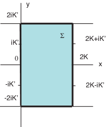
Figure 1: The fundamental domain for $\Sigma$.

5.2 Asymptotic regions and boundary conditions

The poles of $h$ arise when the denominator of (5.7) vanishes, which requires ${\rm\,cn}(y,k^{\prime})=0$ and ${\rm\,sn}(x,k)=0$. Thus, there are no poles on the inside of $\Sigma$. On the boundary $\partial\Sigma$, there are four distinct poles, namely at the points,

$$z_{1}=+iK^{\prime} z_{3}=2K+iK^{\prime}$$

$$z_{2}=-iK^{\prime} z_{4}=2K-iK^{\prime}$$ (5.10)

To investigate the boundary conditions, we evaluate $G$ on the two disjoint boundary components, parametrized by $z=iy$ and $z=2K+iy$ both for $|y|\leq 2K^{\prime}$. The expressions for $G$ are, respectively,

$$G(z=iy) = {{\rm\,cn}(y,k^{\prime})\over|{\rm\,cn}(y,k^{\prime})|}\Big{(}-(B_{1}-B_{1}^{*})-(B_{2}-B_{2}^{*})\Big{)}$$

$$G(z=2K+iy) = {{\rm\,cn}(y,k^{\prime})\over|{\rm\,cn}(y,k^{\prime})|}\Big{(}+(B_{1}-B_{1}^{*})-(B_{2}-B_{2}^{*})\Big{)}$$ (5.11)

Here, we have applied a number of simplifications, made with the help of relations (5.8), as well as using the fact that ${\rm\,dn}(y,k^{\prime})>0$ for all real $y$. Clearly, the real parts of $B_{1}$ and $B_{2}$ are unconstrained by the boundary conditions, and the overall sign of the boundary conditions may be reversed by reversing the imaginary parts of $B_{1}$ and $B_{2}$. Thus, without loss of generality, we may choose $G(z=0)=+i$, which will imply that $G=+i$ for $z=iy$ and $|y|<K^{\prime}$ and $G=-i$ for $z=iy$ and $K^{\prime}<|y|<2K^{\prime}$. With this choice, we now have two possibilities left,

$$G(z=2K)=+i B_{1}^{*}=B_{1}\qquad\qquad B_{2}^{*}-B_{2}=+i$$

$$G(z=2K)=-i B_{2}^{*}=B_{2}\qquad\qquad B_{1}^{*}-B_{1}=+i$$ (5.12)

Note that the entire boundary behavior is generated by either the $B_{1}$ terms, or the $B_{2}$ terms, but not both at the same time.

5.3 The constraint $|G|^{2}>1$

Systematic numerical analysis shows that with the above boundary conditions, the quadratic constraint $|G|^{2}>1$ is obeyed for all $z\in\Sigma$, if and only if either $B_{1}=0$, or $B_{2}=0$. In particular, whenever $B_{1}$ and $B_{2}$ are both non-zero, there is always a region of $\Sigma$ where $|G|<1$. In fact, we find an even stronger result, namely that whenever $B_{1}$ and $B_{2}$ are non-zero, there exists at least one point $z_{0}\in\Sigma$ where $G(z_{0})=0$.

It is possible to prove the above result analytically in the special case of small deformations away from the M-Janus solution. These are achieved, for example, by keeping $B_{1}$ fixed, and taking $B_{2}$ to be small (compared to $B_{1}$). The $B_{2}$-terms then introduce only small changes in $G$ over most of the fundamental domain, except in the neighborhood of the poles of the $B_{2}$-terms. The function $G$ has the following poles in $\Sigma$,

$$B_{1} z=K,\,K+2iK^{\prime}\equiv K-2iK^{\prime}$$-terms

$$B_{2} z=K+iK^{\prime},\,K-iK^{\prime}$$-terms (5.13)

These poles result, respectively, from the zeros of ${\rm\,cn}$, and ${\rm\,dn}$ in the fundamental domain. Each one of the above points $z$ corresponds to a single term in $G$ being singular. Consider now the behavior of $G$ near the poles of the $B_{2}$-terms, $z_{\pm}=K\pm iK^{\prime}$. Here, we have

$${\rm\,sn}(z_{\pm},k) = 1/k$$

$${\rm\,cn}(z_{\pm},k) = \mp ik^{\prime}/k$$

$${\rm\,dn}(z_{\pm},k) = 0$$ (5.14)

where $k,k^{\prime}>0$, and $k^{2}+(k^{\prime})^{2}=1$. The term in $G$ proportional to $B_{2}^{*}$ is the only one exhibiting a singularity at $z=z_{\pm}$; the term proportional to $B_{2}$ vanishes there, while the terms in $B_{1}$ and $B_{1}^{*}$ are regular and non-zero. The singular and leading finite contributions to $G$ are then given as follows,

$$G=\pm{i\over k^{\prime}}\Big{(}B_{1}(1-k)-B_{1}^{*}(1+k)\Big{)}\pm{iB_{2}^{*}\over k^{\prime}}{1\over\bar{z}-\bar{z}_{\pm}}+{\cal O}\left(|z-z_{\pm}|\right)$$ (5.15)

where we have used ${\rm\,dn}(\bar{z}_{\pm})=\mp ik^{\prime}$. If $0<|B_{2}|\ll|B_{1}|$, this form of $G$ will always have a zero $z_{\pm}^{0}$ in the vicinity of $z_{\pm}$, for which we may write down an explicit formula,

$$z_{\pm}^{0}=z_{\pm}+{2B_{2}\over B_{1}(1+k)-B_{1}^{*}(1-k)}+{\cal O}\left(|B_{2}|^{2}\right)$$ (5.16)

The implicit function theorem guarantees that such a solution will exist at least in an open neighborhood of $B_{2}=0$. (For $B_{2}=0$, the pole would be at $z_{\pm}$, but its residue now vanishes.)

This result demonstrates that there cannot be a smooth deformation away from the M-Janus solution, by a “complex conjugate pair of eigenvalue solution” which satisfies the differential equation for $G$, as well as the quadratic constraint $|G|\geq 1$.

5.4 Real and complex conjugate pair eigenvalues

The one logical possibility still left open by the above negative results is the superposition of the $\Phi$-field of the M-Janus solution (with a pair of complex conjugate eigenvalues of $D^{-1}H$), with the $\Phi$-field associated with two real eigenvalues. We shall continue to take the complex eigenvalues to be at $\kappa=\pm i$, and denote the real eigenvalues $\pm 1/a$, for $a$ real and positive. The corresponding $\Phi$ is then given as follows,

$$\Phi = {A_{+}\over a}(1+a\kappa)^{1\over 2}(1+a\bar{\kappa})^{1\over 2}+{A_{-}\over a}(1-a\kappa)^{1\over 2}(1-a\bar{\kappa})^{1\over 2}$$ (5.17)

$$+B(1+i\kappa)^{1\over 2}(1+i\bar{\kappa})^{1\over 2}+B^{*}(1-i\kappa)^{1\over 2}(1-i\bar{\kappa})^{1\over 2}$$

In $\kappa$-coordinates, the function $G$ is given by $G=2i\partial_{\bar{\kappa}}\Phi$, and we find,

$$G=iA_{+}\left({1+a\kappa\over 1+a\bar{\kappa}}\right)^{1\over 2}-iA_{-}\left({1-a\kappa\over 1-a\bar{\kappa}}\right)^{1\over 2}-B\left({1+i\kappa\over 1+i\bar{\kappa}}\right)^{1\over 2}+B^{*}\left({1-i\kappa\over 1-i\bar{\kappa}}\right)^{1\over 2}$$ (5.18)

The branch points on ${\bf R}$ at $\pm a^{-1}$ are responsible for flipping the signs of the corresponding terms there.

To investigate suitable boundary conditions on $G$ requires disentangling the branch cut in the complex plane. The branch points at $\kappa=\pm a^{-1}$ also produce branch cuts, but these could consistently be taken away from the upper half-plane (as was done when we solved the $AdS_{7}\times S^{4}$ deformations). To this end, we carry out a (partial) uniformization, which unfolds the branch cuts starting at $\kappa=\pm i$, and introduce the variable $u$, related to $\kappa$ by,

$$\kappa(u)={2u\over u^{2}-1}$$ (5.19)

We use the M-Janus parameterization $B=(i+\lambda)/2$, and uniformize the square roots in the parameter $a$ by setting,

$$a={\rm\,sh}(\varphi)\hskip 50.58878pt\varphi>0$$ (5.20)

The relevant quadratic functions in $u$ then factorize as follows,

$$u^{2}\pm 2au-1=\left(u+e^{\pm\varphi}\right)\left(u-e^{\mp\varphi}\right)$$ (5.21)

These points are ordered as follows,

$$-e^{\varphi}<-1<-e^{-\varphi}<e^{-\varphi}<+1<e^{\varphi}$$ (5.22)

The resulting $G$-functions is then given by,

$$G = i{{\bar{u}}^{2}-1\over|u^{2}-1|}\left[A_{+}\left({(u+e^{\varphi})(u-e^{-\varphi})\over({\bar{u}}+e^{\varphi})({\bar{u}}-e^{-\varphi})}\right)^{1\over 2}-A_{-}\left({(u-e^{\varphi})(u+e^{-\varphi})\over({\bar{u}}-e^{\varphi})({\bar{u}}+e^{-\varphi})}\right)^{1\over 2}\right.$$ (5.23)

$$\hskip 72.26999pt\left.-{|u|^{2}+1-\lambda(u-{\bar{u}})\over{\bar{u}}^{2}+1}\right]$$

The boundary of $\Sigma$ is to be at ${\rm Im}(\kappa)=0$, which corresponds precisely to ${\rm Im}(u)=0$. As $u$ proceeds along the real axis, the third term in the brackets is constant, and equal to $-1$. In the first two terms, the functions are piece-wise constant, but change sign whenever a branch cut is being traversed. The basic function to be considered is

$$f(u)=\left({u-u_{0}\over{\bar{u}}-u_{0}}\right)^{1\over 2}$$ (5.24)

where $u_{0}$ is real. Assuming that the sign of the square root is taken to be + for $u>u_{0}$, we determined the sign for $u<u_{0}$ by introducing an adapted local coordinate, $u=u_{0}+v^{2}$, in which we have $f(u)=v/\bar{v}$. As we proceed from $u>u_{0}$ for which $v$ is real so that $f(u)=+1$, to $u<u_{0}$ for which $v$ is imaginary, we see that we must have $f(u)=-1$. Following this procedure through all branch cuts, we have the following table of boundary values of $G$,

$$e^{\varphi}<u~{}~{}~{}~{}~{} G=+i(A_{+}-A_{-}-1)$$

$$+1<u<e^{\varphi} G=+i(A_{+}+A_{-}-1)$$

$$e^{-\varphi}<u<+1 G=-i(A_{+}+A_{-}-1)$$

$$-e^{-\varphi}<u<e^{-\varphi} G=-i(-A_{+}+A_{-}-1)$$

$$-1<u<-e^{-\varphi} G=-i(-A_{+}-A_{-}-1)$$

$$-e^{\varphi}<u<-1 G=+i(-A_{+}-A_{-}-1)$$

$$u<-e^{\varphi}~{}~{}~{}~{}~{} G=+i(A_{+}-A_{-}-1)$$ (5.25)

The overall sign reversals for $-1<u<+1$ are due to the prefactor $({\bar{u}}^{2}-1)/|u^{2}-1|$ in $G$. The boundary conditions require that $G=\pm i$ throughout the real line, or equivalently,

$$(A_{+}\pm A_{-}-1)^{2}=(-A_{+}\pm A_{-}-1)^{2}=1$$ (5.26)

where the above $\pm$ signs are uncorrelated. These conditions require that $A_{+}(\pm A_{-}-1)=0$. Taking the sum of these two relations, we find $A_{+}=0$, and thus $A_{-}=0$. Thus, one cannot add the real eigenvalue contributions without violating the boundary conditions on $G$.

5.5 Generalization to arbitrary numbers of poles

The arguments presented in the preceding sections were for $p=2$ and $q=1$, but may be generalized to arbitrary $p,q$, by considering a solution to the differential equation for $G$ which has $q$ complex conjugate pairs of eigenvalues. For simplicity, we shall limit the discussion here to the case $p=0$. The expression for $G$ is readily written down in terms of the holomorphic function $\kappa$, which runs through the upper half-plane, ${\rm Im}(\kappa)>0$,

$$G=\sum_{n=1}^{N}\left[-B_{n}\left({\kappa-w_{n}\over\bar{\kappa}-w_{n}}\right)^{1\over 2}+B_{n}^{*}\left({\kappa-\bar{w}_{n}\over\bar{\kappa}-\bar{w}_{n}}\right)^{1\over 2}\right]\hskip 43.36243pt{\rm Im}(w_{n})>0$$ (5.27)

The generalization of the preceding result, which had been obtained for the elliptic case only, may be stated as follows.

For sufficiently small $B_{m}$ the singularity at $\kappa=w_{m}$ is a pole which produces a zero of $G$ in its neighborhood.

To prove this, we begin by uniformizing the square root around $w_{m}$, in a neighborhood of $w_{m}$, and introduce a suitable local coordinate $u$,

$$\kappa-w_{m}=u^{2}$$ (5.28)

The singular and leading finite contributions to $G$ are then given as follows,

$$G = G_{m}+B_{m}^{*}{\sqrt{w_{m}-\bar{w}_{m}}\over\bar{u}}$$

$$G_{m} = \sum_{n\not=m}\left[-B_{n}\left({w_{m}-w_{n}\over\bar{w}_{m}-w_{n}}\right)^{1\over 2}+B_{n}^{*}\left({w_{m}-\bar{w}_{n}\over\bar{w}_{m}-\bar{w}_{n}}\right)^{1\over 2}\right]$$ (5.29)

For each $m$, the quantity $G_{m}$ is a finite complex number. If $G_{m}$ happens to vanish (which is not generic), then $B_{m}=0$ produces a zero of $G$. If $G_{m}\not=0$, then $G$ has a zero in the neighborhood of $w_{m}$, for which we may give an explicit formula,

$$u=B_{m}{\sqrt{\bar{w}_{m}-w_{m}}\over G_{m}^{*}}+{\cal O}\Big{(}|B_{m}|^{2}\Big{)}$$ (5.30)

Thus, we conclude that, within the approximation of small deviations away from the maximally symmetric solution, the bound $|G|>1$ is always violated by a region containing a point where $G=0$.

6 M-brane interpretation of rigidity

There are several arguments in M-theory for the existence of half-BPS brane configurations whose geometry is $AdS_{3}\times S^{3}\times S^{3}$ warped over a two-dimensional surface $\Sigma$. We list these arguments below, and discuss their various qualifications and limitations.

• The first argument originates from considering the symmetries of probe branes, such as M2 probe branes inserted into $AdS_{7}\times S^{4}$, or M5 probe branes inserted into $AdS_{4}\times S^{7}$. The embedding of the probe branes preserves the same symmetries as our Ansatz for full solutions does. The preservation of half of the supersymmetries of the probe branes is assured, in the Green-Schwarz formalism, by the existence of a kappa-symmetry projector in the world-volume theory of the probe brane [34]. While the presence of probe branes is suggestive of the existence of back-reacted supergravity solutions, only the resolution of the full supergravity BPS equations (as is being analyzed here) can conclusively decide on the existence of any full fledged regular supergravity solutions.

• The second argument rests on the existence of asymptotic symmetries and supersymmetries in AdS space-times. The existence of full fledged half-BPS supergravity solutions with local $AdS_{4}\times S^{7}$ asymptotics requires the existence of certain subalgebras with 16 fermionic generators of $OSp(8|4,{\bf R})$. These subalgebras do indeed exist [13]. Conversely, however, the mere existence of a corresponding subalgebra does not suffice to guarantee existence of a full-fledged regular supergravity solution.

• The third argument is based on the expected symmetry enhancement, in the near-horizon limit, for the 1+1 dimensional intersection of M2- and M5-branes. The full regular supergravity solution with M2- and M5-branes intersecting over a 1+1-dimensional space-time is expected to exist and preserve 1/4 of the supersymmetries of flat space-time. Enhancement in the near-horizon limit would then result in a regular half-BPS supergravity solution. Note, however, that no such localized intersecting brane solutions are known explicitly at this time, so that we do not know for sure which near-horizon limits exist, and which do not. Thus, the third argument proceeded mostly by analogy with known cases in Type IIB, but does not guarantee existence of full fledged regular supergravity solutions either.

All three arguments given above would proceed in parallel for the cases of solutions asymptotic either to $AdS_{4}\times S^{7}$ or to $AdS_{7}\times S^{4}$. The arguments would suggest the existence of full fledged half-BPS solutions asymptotic to $AdS_{4}\times S^{7}$ just as they do for solutions asymptotic to $AdS_{7}\times S^{4}$. Having critically discussed the various arguments above in favor of the existence of regular supergravity solutions with $AdS_{4}\times S^{7}$ asymptotics, we shall now refine the arguments by exhibiting a fundamental asymmetry between the case of solutions asymptotic to $AdS_{4}\times S^{7}$ and the case asymptotic to $AdS_{7}\times S^{4}$. This asymmetry will be key in our final argument against the existence of regular half-BPS supergravity solutions which are asymptotic to $AdS_{4}\times S^{7}$ and carry M5-brane charges.

6.1 Asymmetry between M2- and M5- branes

The conserved charges associated with M5- and M2-branes are given by,

$$Q_{5}=\int_{{\cal M}_{4}}F_{4},\hskip 72.26999ptQ_{2}=\int_{{\cal M}_{7}}(*F_{4}+F_{4}\wedge C_{3})$$ (6.1)

where ${\cal M}_{4}$ and ${\cal M}_{7}$ are surfaces surrounding the M5- and M2-brane, respectively, capturing all the flux. From the arguments given at the beginning of this section one would naively expect that there exist two kinds of half-BPS solutions: First, fully back-reacted solutions asymptotic to $AdS_{7}\times S^{4}$ which also support M2-brane charge and second, fully back-reacted solutions asymptotic to $AdS_{4}\times S^{7}$ which also support M5-brane charge.

Solutions corresponding to the first case do indeed exist and were explicitly constructed in [22]. These solutions have one asymptotic $AdS_{7}\times S^{4}$ region and in addition non-trivial seven cycles with non-zero $Q_{2}$.

The arguments and calculations presented in the present paper show, however, that the corresponding solutions for the second case do not exist. In other words, even though the general fully back-reacted half-BPS solution which is asymptotic to $AdS_{4}\times S^{7}$ has non-trivial 4-cycles, they do not support any net M5-brane charge. In fact, the only new half-BPS solution found here and in [23] is the M-Janus solution and its multiple covers, but these solutions have no net M5-brane charges.

The asymmetry of the two cases may seem surprising at first , given the fact that the local solutions are very similar. In the following we give an explanation for the different behavior of the two cases. Two key Theorems enter into consideration,

Theorem 1

M2-branes can end on M5-branes, but M5-branes cannot end on M2-branes.

Theorem 2

No solutions exist which have $SO(2,2)\times SO(4)\times SO(4)$ symmetry and 16 supersymmetries throughout space-time and possess both $AdS_{4}\times S^{7}$ and $AdS_{7}\times S^{4}$ asymptotic regions.

The result of Theorem 1 dates back to the early days of M-theory (see for example [35, 36]), and was obtained using the Chern-Simons term in M-theory. The argument for why an M5-brane can not end on an M2-brane is as follows. The 4-surface ${\cal M}_{4}$ in the formula (6.1) for the M5-brane charge surrounds the M5-brane transversely to capture all the flux. If the M5-brane ends on an M2-brane, this surface can be slipped off and contracted and we arrive at a contradiction, since one calculation of the M5-brane charge gives a non-zero while the other calculation gives zero.

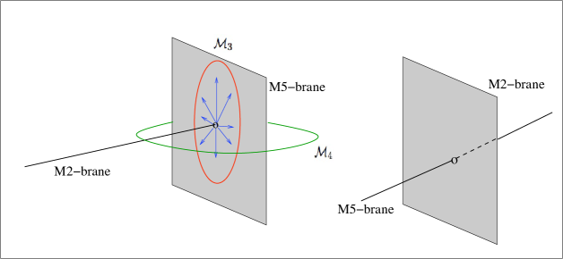
Figure 2: An M2-brane ending on an M5-brane produces flux inside the M5-brane worldvolume. By contrast, an M5-brane can only intersect an M2 brane (see also [36]).

The existence of a Chern-Simons term in the 11-dimensional supergravity action implies the presence of the $F_{4}\wedge C_{3}$ term in the formula for the M2-brane charge (6.1). This term makes it possible for an M2-brane to end on an M5-brane without violating charge conservation. As one tries to slip off the seven surface ${\cal M}_{7}$ in (6.1), the surface decomposes into a 4-surface ${\cal M}_{4}$ enclosing the M5-brane on which the M2-brane ends and a 3-surface ${\cal M}_{3}$ lying in the world-volume of the M5-brane enclosing the two dimensional boundary of the M2-brane,

$$Q_{2}=\int_{{\cal M}_{4}}F_{4}\int_{{\cal M}_{3}}C_{3}=Q_{5}\int_{{\cal M}_{3}}C_{3}$$ (6.2)

An M2-brane ending on a M5-brane induces a non-trivial 3-form field $C_{3}$ in the world-volume of the M5-brane. This supergravity field is related to the self-dual 3-form field strength of the world-volume theory of the M5-brane [37, 38, 39].

The result of Theorem 2 was obtained in [14], and derived from the explicit construction of the local solutions. The general half-BPS solution is characterized by three real constants $c_{i},i=1,2,3$, which are subject to the condition $c_{1}+c_{2}+c_{3}=0$. The constants $c_{i},i=1,2,3$ are related to the normalization of the metrics of the $AdS_{3}\times S^{3}\times S^{3}$ factors respectively. An overall scaling of all $c_{i}$ can be absorbed into a rescaling of the eleven dimensional metric and is not important. The key fact is that the choice of $c_{i}$ characterizes the asymptotic geometry of the half-BPS solution completely. In particular the choices $c_{1}=c_{2}$ and $c_{1}=c_{3}$ imply asymptotic $AdS_{7}\times S^{4}$ regions, whereas $c_{2}=c_{3}$ implies asymptotic $AdS_{4}\times S^{7}$ regions. Because of the $c_{1}+c_{2}+c_{3}=0$ constraint the conditions can never be satisfied simultaneously. It follows that a half BPS-solution cannot have asymptotic $AdS_{7}\times S^{4}$ and $AdS_{4}\times S^{7}$ regions at the same time.

6.2 Comparison to solutions asymptotic to $AdS_{7}\times S^{4}$

The argument presented above shows that if an M2-brane ends on (a stack of) M5-branes, the net flux carried by the M2-brane is conserved and must be carried off by the gauge field on the M5-brane. No matter which limit we take of the M5-brane (such as the near-horizon limit), the net flux will continue to produce a non-zero M2-brane charge on the M5-brane. Therefore, in the near-horizon limit, we should expect to recover an $AdS_{7}\times S^{4}$ space-time with net M2-brane charges inserted at the remnant points due to the M2-branes. This is indeed borne out by the explicit and exact solutions of [22], which exhibit net M2-brane charges in an asymptotic $AdS_{7}\times S^{4}$ space-time.

Theorem 2 implies that, given the $AdS_{7}\times S^{4}$ asymptotic solution with non-trivial M2-brane charges, there should exist no limit in which we can recover the M2-brane geometry. Indeed, if such a M2-brane near-horizon limit existed, then we would have a geometry which exhibits both an $AdS_{4}\times S^{7}$ asymptotic region (namely near the M2-brane) and an $AdS_{7}\times S^{4}$ asymptotic region (namely space-time away from the M2-brane insertions), but this is impossible in view of Theorem 2. This result is also borne out by the explicit solution of [22]. Its only moduli are the positions $x_{m}$ of the sign-flips in $G$ on the boundary of $\Sigma$. Thus, the only limits we can consider is to let consecutive positions $x_{m}$ collapse to one another.

We compute explicitly the M2-charges and show a singular M2-brane never emerges in the limit of collapsing moduli. Using the general expression for $G$ in (3.28) of [22], as well as the expressions for the fluxes in (2.8) of [22], we may compute the explicit fluxes in an asymptotic expansion away from the boundary for the case of general $g$. The result is

$$\partial_{w}b_{i}=-2i\varepsilon_{i}-i\eta_{i}\sum_{n=1}^{g+1}\bigg{(}{x-x_{2n-1}\over|x-x_{2n-1}|}-{x-x_{2n}\over|x-x_{2n}|}\bigg{)}+{\cal O}(y)$$ (6.3)

The values of the sign factors $\varepsilon_{i}$ and $\eta_{i}$ are given by $\varepsilon_{1}=-\varepsilon_{2}=+1$, $\varepsilon_{3}=0$, and $\eta_{1}=\eta_{2}=-\eta_{3}=1$, and the points are ordered as follows,

$$x_{1}<x_{2}<x_{3}<\cdots<x_{2g}<x_{2g+1}<x_{2g+2}$$ (6.4)

In general, the geometry contains $2g+1$ four-cycles, which split into two groups. One group contains $g$ four-cycles formed from the first three sphere $S_{2}^{3}$, while the second group contains $g+1$ four-cycles formed from the second sphere $S_{3}^{3}$. The charge along the first group can be computed by integrating the imaginary part of $\partial_{w}b_{2}$ along the boundary starting from $\xi_{n}$ and ending at $\xi_{n+1}$ with $n=1,...,g$ and $x_{2n-1}<\xi_{n}<x_{2n}$. The charge along the second group of four cycles can be computed by integrating the imaginary part of $\partial_{w}b_{3}$ along the boundary starting from $\xi^{\prime}_{n}$ and ending at $\xi^{\prime}_{n+1}$ with $n=0,...,g$ and $x_{2n}<\xi^{\prime}_{n}<x_{2n+1}$. Here we take $x_{0}=-\infty$ and $x_{2g+3}=+\infty$. The resulting charges are independent of the choices for $\xi_{n}$ and $\xi^{\prime}_{n}$ and are given as

$$Q_{5n}^{(2)} = q_{5}^{(2)}(x_{2n+1}-x_{2n})\qquad n=1,...,g$$

$$Q_{5n}^{(3)} = q_{5}^{(3)}(x_{2n}-x_{2n-1})\qquad n=1,...,g+1$$ (6.5)

where $Q_{5n}^{(2)}$ is the charge along $S^{3}_{2}$ and $Q_{5n}^{(3)}$ is the charge along $S^{3}_{3}$. Here, $q_{5}^{(2)}$ and $q_{5}^{(3)}$ are constants, i.e. parameters which are independent of the points $x_{n}$. Taking $x_{2n+1}\rightarrow x_{2n}$ we see that $Q_{5n}^{(2)}\rightarrow 0$ while taking $x_{2n}\rightarrow x_{2n-1}$ we see that $Q_{5n}^{(3)}\rightarrow 0$.

To compute the M2-brane charge, we first note that the integral of $*F_{4}$ over the seven cycle formed by the product of one of the four-cycles and the conjugate three sphere always vanishes. This is because we must integrate the real part of $\partial_{w}b_{1}$ along the boundary which always vanishes. This shows that the M2-brane charge comes purely from the topological term and takes the value

$$Q_{2i}^{(2)}=\int_{S^{4}_{2i}}F_{4}\int_{S^{3}_{3}}C_{3}=Q_{5i}^{(2)}\int_{S^{3}_{3}}C_{3}$$

$$Q_{2i}^{(3)}=\int_{S^{4}_{3i}}F_{4}\int_{S^{3}_{2}}C_{3}=Q_{5i}^{(3)}\int_{S^{3}_{2}}C_{3}$$ (6.6)

Collapsing branch cuts, we see that the vanishing of the M5-charge immediately implies the vanishing of the M2-charge. Thus, in the limit consecutive positions $x_{m}$ collapse to one another we see that the net M2-brane charge localized at these points always tends to 0.

6.3 Completing arguments for solutions asymptotic to $AdS_{4}\times S^{7}$

The arguments for the absence of half-BPS solutions which are asymptotic to $AdS_{4}\times S^{7}$ and support M5-brane charge can now be completed.

Theorem 1, given above, asserts that an M5-brane cannot end on an M2-brane. Hence there is no net 4-form flux to fan out into the M2-brane geometry that produces a non-vanishing net M5-brane charge. Of course, the M5-brane can simply intersect the M2-brane, but this configuration produces no net charge into the M2-brane. In the near-horizon limit, no M5-brane flux is required to survive.

Theorem 2, given above, implies that there exists no near-horizon limit in which both the M2-brane and the M5-brane survive (since this limit would exhibit both $AdS_{4}\times S^{7}$ and $AdS_{7}\times S^{4}$ asymptotic regions). Hence, the near-horizon limit will be either that of an M2-brane or of an M5-brane, but not of both simultaneously. This implies that the $AdS_{4}\times S^{7}$ asymptotic space-time cannot sustain any conserved 5-brane charge.

These arguments seem to be borne out by the fact that on the one hand the explicit solutions we have found in this paper, i.e. the multi cover M-Janus solutions of section 3, have four cycles and a nontrivial 4-form field, but that on the other hand the integrated M5-brane charge along these cycles vanishes. We discuss possibles loopholes in this result in the next section.

7 Discussion

The main result of the present paper is that regular half BPS-solutions of M-theory that enjoy $SO(2,2)\times SO(4)\times SO(4)$ symmetry and are asymptotic to $AdS_{4}\times S^{7}$ are remarkably rigid in the sense that the only non-trivial solutions we have found is the M-Janus solution of [23] and multiple covers thereof. We have given an interpretation of this result in terms of M2- and M5-brane intersections and endings in the previous section. In this section, we shall conclude with a discussion of a number of questions left open by our work, and of possible directions for further research.

7.1 Origin and physical significance of multiple covers of M-Janus

The first open question concerns the physical interpretation of the multiple covers of the M-Janus solution found in section 3. The M-Janus solution [23] has two asymptotic $AdS$ regions. Its interpretation in the dual 2+1-dimensional CFT is given by the insertion of a dimension 2 operator localized along a 1+1-dimensional linear interface/defect, thereby partially breaking the superconformal symmetry. The $(g+1)$-fold cover of the M-Janus solution in turn has $2g+2$ asymptotic $AdS$ regions. The behavior of the supergravity fields is identical to that of the parent M-Janus solution with only two asymptotic regions, and can in principle be smoothly projected to the parent M-Janus solution by a freely acting discrete transformation group. Furthermore, the solution does not support any M5-brane charge.

It is useful to contrast this solution with the corresponding multi-Janus solution of Type IIB supergravity which was constructed in [26]. The Type IIB multi-Janus solution also has $2g+2$ asymptotic $AdS$ regions. However, in the Type IIB solution, the dilaton generically takes different values in the different asymptotic regions. In the dual CFT this means that the theories on the different half-spaces, which are glued together at the defect, are all different. In addition, the solution supports non-zero five brane charge. In M-theory, the bulk CFTs dual to each asymptotic region have no free parameters, since the gauge coupling of the maximally supersymmetric 2+1-dimensional CFT is fixed. This may be the source of the identical nature of the cover copies in the corresponding supergravity solutions.

It would be interesting to investigate the multiple cover solutions further. On the supergravity side it is possible to calculate correlation functions of operators located in different asymptotic regions, and elucidate whether the multiple-cover M-Janus solutions are genuinely different from the parent solutions with only two asymptotic $AdS$ regions. It would also be interesting to determine whether a sensible CFT interpretation of the multiple defect theories exists.

A great deal of progress has been made in understanding the CFT associated with the decoupling limit of multiple M2-branes [9, 10, 11]. Of particular interest is the ABJM solution of [12] which has manifest ${\cal N}=6$ supersymmetry and is dual to M-theory on the quotient $AdS_{4}\times S^{7}/Z_{k}$. The M-Janus solution admits a regular ABJM reduction to a quotient solution which is invariant under $SO(2,2)\times SO(4)\times U(1)^{2}$, preserves 12 supersymmetries, and provides a Janus-like interface/defect solution in ABJM theory. It would be interesting to analyze the multiple cover M-Janus solution and its dual CFT interpretation in the context of the ABJM quotient as well.

7.2 Can one relax the regularity and boundary conditions ?

The second open question concerns the assumptions we have made on the boundary and regularity conditions. The rigidity result we found is closely related to the regularity assumptions and the constraint $|G|^{2}>1$, which the solution has to satisfy point-wise. It is easy to construct more general solutions which satisfy the differential equation (4.17) by linear superposition. In all the cases we have explored, however, the solution has one or more of the following properties:

1. the solution is singular;

2. the solution is not asymptotic to $AdS_{4}\times S^{7}$;

3. the solution violates the constraint $|G|^{2}>1$.

It is an open question wether it is possible to modify or omit some of the assumptions in order to obtain new solutions which have a sensible physical interpretation. Below, we shall list three scenarios in which weaker conditions appear.

$\bullet$ First, there exists an example of such a solution in the literature [15, 16, 17] which violates assumption 2. It is characterized by a space-time manifold $AdS_{3}\times S^{3}\times S^{3}\times T^{2}$ without any warping. The solution is regular, but not asymptotic to $AdS_{4}\times S^{7}$. A systematic analysis of more general solutions with other asymptotics would be interesting, but is beyond the scope of this paper.

$\bullet$ Second, the absence of any M5-brane charge in our regular solutions may suggest that if one drops the condition of regularity on the boundary $\partial\Sigma$, it might be possible to obtain solutions which have non vanishing M5-brane charge. A particular generalization is obtained by choosing a harmonic function $h$ of the type given in (3.5), but which contains higher order poles. Another possibility is to allow for isolated points on the inside of $\Sigma$ where the constraint $|G|^{2}>1$ is violated, and we have instead $|G|^{2}=1$. It is an open question whether such solutions are sensible. One possibility is that singular solutions may be associated with the presence of probe M5-branes in the $AdS_{4}\times S^{7}$ spacetime.

$\bullet$ Last, it might be the case that demanding the preservation of 16 supersymmetries is too restrictive to allow for regular solutions. A way out might be to look for solutions which only preserve 8 supersymmetries, yielding quarter-BPS solutions. Intersecting M2/M5-brane solutions in flat space preserve one quarter of the 32 Minkowski supersymmetries and it is possible that the near-horizon limit does not lead to an enhancement of the number of supersymmetries from 8 to 16. We leave these interesting questions for future work.

Acknowledgements

MG gratefully acknowledges the hospitality of the Department of Physics and Astronomy, Johns Hopkins University, during the course of this work.

Appendix A Reduced form of the polynomial $P$

The form of the polynomial $P$ in the Ansatz of (3.16) does not account for the most general real polynomial of degree 4. In this appendix, we shall derive the general restrictions on $P$ of (3.9) that result from the polynomial equations (3.10) and the boundary conditions. To construct explicit solutions, and describe their moduli spaces concretely, it will be helpful to reduce the Ansatz of (3.9) by demonstrating that $P$ is not a general polynomial of degree $2g+2$ in $u,{\bar{u}}$, but obeys certain restrictions, as a consequence of the boundary conditions and of the polynomial equation (3.10).

$\bullet$ The boundary conditions force $P$ to consist of an arbitrary polynomial of degree $2g+1$ plus a single term of the form $(u\bar{u})^{g+1}$. To obtain this result, we note that $u\to\infty$ is part of the boundary of $\Sigma$ on which we must have $|G|=1$. The magnitude of $G$ may be readily evaluated from (4.17). The asymptotic behavior as $u\to\infty$ of the denominator of $G$ is,

$$\bar{Q}\partial_{\bar{u}}\bar{R}-\bar{R}\partial_{\bar{u}}\bar{Q}=(2g+1)\bar{u}^{4g+2}\sum_{i=1}^{2g+2}c_{i}$$ (A.1)

Considering now the behavior of a term $P_{mn}=u^{m}\bar{u}^{n}\pm u^{n}{\bar{u}}^{m}$ in $P$ as $u\rightarrow\infty$, we find,

$$P_{mn}\partial_{\bar{u}}\bar{Q}-2\bar{Q}\partial_{\bar{u}}P_{mn}=(2g+2-2n)u^{m}\bar{u}^{n+2g+1}\pm(2g+2-2m)u^{n}\bar{u}^{m+2g+1}$$ (A.2)

Requiring the ratio of the numerator and the denominator of the expression for $|G|$ to be finite as $u\to\infty$ yields the following allowed orders $m,n$,

$$m=n = g+1$$

$$m+n \leq 2g+1$$ (A.3)

which proves our above assertion.

$\bullet$ The polynomial relation (3.10) will schematically be represented by ${\cal D}P=0$. This relation forces further restrictions. It will be instructive to derive these independently of the restrictions derived above from the boundary conditions. The most general real polynomial $P$ of degree $2g+2$ in $u,{\bar{u}}$, may be parametrized as follows,

$$P(u,\bar{u})=\sum_{m=0}^{2g+2}\sum_{{0\leq n\leq m\atop m+n\leq 2g+2}}\!\!\!d_{m,n}(u^{m}\bar{u}^{n}+u^{n}\bar{u}^{m})+\sum_{m=0}^{2g+2}\sum_{{0\leq n\leq m-1\atop m+n\leq 2g+2}}\!\!\!ie_{m,n}(u^{m}\bar{u}^{n}-u^{n}\bar{u}^{m})$$ (A.4)

The polynomial $P$ is real provided $d_{m,n}$ and $e_{m,n}$ are real. The number of free parameters for $d_{m,n}$ is $(g+2)(2g+3)$, while for $e_{m,n}$, it is $(g+1)(2g+3)$, giving a total of $(2g+3)^{2}$. Parts of the polynomial relation ${\cal D}P(u,{\bar{u}})=0$ may be solved by an iterative process.

The following restrictions are found to arise,

1. All coefficients $d_{m,n}$ with $m>g+1$ must vanish;

2. All coefficients $e_{m,n}$ must vanish.

These results may be shown iteratively beginning with the coefficients corresponding to the highest value of $m-n$, which are $d_{2g+2,0}$ and $e_{2g+2,0}$. Equations in which these coefficients appear as overall factors, show that these coefficient must vanish. Setting now $d_{2g+2,0}=e_{2g+2,0}=0$, one finds that there are factorized equations also for $d_{2g,2}$ and $e_{2g,2}$, so that also these coefficients must vanish and so on. In this manner, one shows iteratively that $d_{m,n}=e_{m,n}=0$ for all $m>g+1$. (Note that the coefficients $d_{m,n}$ and $e_{m,n}$ are defined with $m\geq n$, so that $n>g+1$ automatically implies $m>g+1$, and these cases does not have to be considered separately.)

To show that the coefficients $e_{m,n}$ for the remaining range of $m,n$ also vanish, one proceeds to split the polynomial relation ${\cal D}P(u,{\bar{u}})$ into real and imaginary parts. These are correlated with the appearance of the coefficients $d_{m,n}$ and $e_{m,n}$, as follows,

$$({\cal D}P)(u,{\bar{u}})-({\cal D}P)({\bar{u}},u) d_{m,n}$$ contains only

$$({\cal D}P)(u,{\bar{u}})+({\cal D}P)({\bar{u}},u) e_{m,n}$$ contains only (A.5)

The vanishing of all contributions containing only $e_{m,n}$ may be solved iteratively again, each time encountering at least one coefficient $e_{m,n}$ in factorized form. We have checked these results explicitly by MAPLE for $g=0,1,2,3,4$.

In summary, incorporating the above results, the form of the polynomial Ansatz is drastically simplified, and we are left with the following remaining form,

$$P(u,\bar{u})=\sum_{m=0}^{g+1}\,\sum_{n=0}^{m}d_{m,n}\left(u^{m}\bar{u}^{n}+u^{n}\bar{u}^{m}\right)$$ (A.6)

Note that the term of maximal degree is unique, and given by $2d_{m,m}(u{\bar{u}})^{m}$ with $m=g+1$. As a result, the point $u=\infty$ is a regular point of the functions $\Phi$ and $G$.

Appendix B Derivation of the complex analytic equations

In this section, we shall show that the assumption of Hermitian pairing in (4.1) together with the boundary conditions of (4.2) leads to a Cauchy-Riemann type differential equation for the functions $\phi_{m}$, given in (4.3). We shall now proceed to reducing the partial differential equations to a set of differential equations in just the holomorphic coordinate $u$. This reduction is general, and will be proven with the help of a Lemma below.

Lemma 1

Let $\xi_{m}(u)$ and $\zeta_{m}(u)$ with $m=1,\cdots,N$ be meromorphic functions of $u$, and let the set $\{\xi_{m}(u)\}$ consist of $N$ linearly independent functions. Both $\xi_{n}(u)$ and $\zeta_{m}(u)$ are assumed to be real, in the sense that $\overline{\xi_{m}(u)}=\xi_{m}({\bar{u}})$ and $\overline{\zeta_{m}(u)}=\zeta_{m}({\bar{u}})$. If the following pairing

$$\sum_{m=1}^{N}\overline{\zeta_{m}(u)}\xi_{m}(u)$$ (B.1)

is real for all complex $u$, then there exists a real symmetric $N\times N$ matrix $H$, whose coefficients are independent of $u,{\bar{u}}$, such that

$$\zeta_{m}(u)=\sum_{n=1}^{N}H_{mn}\xi_{n}(u)$$ (B.2)

To prove the Lemma, we make use of the reality of the functions to express the complex conjugates $\overline{\zeta_{m}(u)}$ of the function $\zeta_{m}(u)$ in terms of the same function $\zeta_{m}(v)$ evaluated on the complex conjugate variable $v={\bar{u}}$ instead. The reality condition of the pairing may then be written as follows,

$$\sum_{m=1}^{N}\Big{(}\zeta_{m}(v)\xi_{m}(u)-\zeta_{m}(u)\xi_{m}(v)\Big{)}=0$$ (B.3)

As usual, we may now view $v$ as a complex variable which is completely independent of $u$. We may now regard the functions $\xi_{m}(u)$ as a given set of linearly independent meromorphic functions, and seek to establish the relation of the $\zeta_{m}$-functions with $\xi_{m}$. The linear independence of the functions $\xi_{m}(u)$ for $m=1,\cdots,N$ guarantees that we can pick $N$ points $a_{n}$ with $n=1,\cdots,N$ such that the $N\times N$ matrix $\xi_{m}(a_{n})$ is invertible. We denote its inverse by $X_{mn}$, so that

$$\sum_{p=1}^{N}\xi_{m}(a_{p})X_{pn}=\delta_{mn}$$ (B.4)

Hence, we have

$$\zeta_{m}(u)=\sum_{n=1}^{N}H_{mn}\xi_{n}(u)\hskip 72.26999ptH_{mn}=\sum_{p=1}^{N}\zeta_{n}(a_{p})X_{pm}$$ (B.5)

The matrix $H$ is independent of $u$ by construction. It is also independent of the choice of points $a_{p}$. A non-zero meromorphic function cannot vanish identically on the real axis. Therefore, the points $a_{p}$ may be chosen on the real axis, and thus $H_{mn}$ is real. That the matrix $H$ is also symmetric may be established by substituting the relation $\zeta=H\xi$ back into the equation, which gives,

$$\sum_{m,n=1}^{N}H_{mn}\Big{(}\xi_{m}(u)\xi_{n}(v)-\xi_{m}(v)\xi_{n}(u)\Big{)}=0$$ (B.6)

Only the anti-symmetric part of $H$ contributes in this equation. If the anti-symmetric part were non-zero, the equation, for any fixed $v$, would imply a non-trivial linear relation between the functions $\xi_{m}(u)$. Since the $\xi_{m}$ were assumed to be linearly independent, such a relation must be trivial, forcing $H_{mn}-H_{nm}=0$.

References

- [1]
- [2] J. M. Maldacena, “The large N limit of superconformal field theories and supergravity,” Adv. Theor. Math. Phys. 2 (1998) 231 [Int. J. Theor. Phys. 38 (1999) 1113] [arXiv:hep-th/9711200].
- [3] S. S. Gubser, I. R. Klebanov and A. M. Polyakov, “Gauge theory correlators from non-critical string theory,” Phys. Lett. B 428 (1998) 105 [arXiv:hep-th/9802109].
- [4] E. Witten, “Anti-de Sitter space and holography,” Adv. Theor. Math. Phys. 2 (1998) 253 [arXiv:hep-th/9802150].
- [5] O. Aharony, S. S. Gubser, J. M. Maldacena, H. Ooguri and Y. Oz, “Large N field theories, string theory and gravity,” Phys. Rept. 323 (2000) 183 [arXiv:hep-th/9905111].
- [6] E. D’Hoker and D. Z. Freedman, “Supersymmetric gauge theories and the AdS/CFT correspondence,” in Strings, Branes, and Extra Dimensions, S.S. Gubser, J.D. Lykken, Eds, World Scientific (2004), arXiv:hep-th/0201253.
- [7] O. Aharony, Y. Oz and Z. Yin, “M-theory on AdS(p) x S(11-p) and superconformal field theories,” Phys. Lett. B 430 (1998) 87 [arXiv:hep-th/9803051].
- [8] S. Minwalla, “Particles on AdS(4/7) and primary operators on M(2/5) brane world-volumes,” JHEP 9810 (1998) 002 [arXiv:hep-th/9803053].
- [9] J. Bagger and N. Lambert, “Modeling multiple M2’s,” Phys. Rev. D 75 (2007) 045020 [arXiv:hep-th/0611108].
- [10] J. Bagger and N. Lambert, “Gauge Symmetry and Supersymmetry of Multiple M2-Branes,” Phys. Rev. D 77 (2008) 065008 [arXiv:0711.0955 [hep-th]].
- [11] A. Gustavsson, “Algebraic structures on parallel M2-branes,” Nucl. Phys. B 811 (2009) 66 [arXiv:0709.1260 [hep-th]].
- [12] O. Aharony, O. Bergman, D. L. Jafferis and J. Maldacena, “N=6 superconformal Chern-Simons-matter theories, M2-branes and their gravity duals,” JHEP 0810, 091 (2008) [arXiv:0806.1218 [hep-th]].
- [13] E. D’Hoker, J. Estes, M. Gutperle, D. Krym and P. Sorba, “Half-BPS supergravity solutions and superalgebras,” JHEP 0812 (2008) 047 [arXiv:0810.1484 [hep-th]].
- [14] E. D’Hoker, J. Estes, M. Gutperle and D. Krym, “Exact Half-BPS Flux Solutions in M-theory I, Local Solutions,” JHEP 0808 (2008) 028 [arXiv:0806.0605 [hep-th]].
- [15] H. J. Boonstra, B. Peeters and K. Skenderis, “Brane intersections, anti-de Sitter spacetimes and dual superconformal theories,” Nucl. Phys. B 533 (1998) 127 [arXiv:hep-th/9803231].
- [16] J. P. Gauntlett, R. C. Myers and P. K. Townsend, “Supersymmetry of rotating branes,” Phys. Rev. D 59 (1999) 025001 [arXiv:hep-th/9809065].
- [17] J. de Boer, A. Pasquinucci and K. Skenderis, “AdS/CFT dualities involving large 2d N = 4 superconformal symmetry,” Adv. Theor. Math. Phys. 3 (1999) 577 [arXiv:hep-th/9904073].
- [18] J. P. Gauntlett, O. A. P. Mac Conamhna, T. Mateos and D. Waldram, “New supersymmetric AdS(3) solutions,” Phys. Rev. D 74 (2006) 106007 [arXiv:hep-th/0608055].
- [19] A. Donos, J. P. Gauntlett and N. Kim, “AdS Solutions Through Transgression,” JHEP 0809, 021 (2008) [arXiv:0807.4375 [hep-th]].
- [20] S. Yamaguchi, “Bubbling geometries for half-BPS Wilson lines,” Int. J. Mod. Phys. A 22 (2007) 1353 [arXiv:hep-th/0601089].
- [21] O. Lunin, “1/2-BPS states in M theory and defects in the dual CFTs,” JHEP 0710 (2007) 014 [arXiv:0704.3442 [hep-th]].
- [22] E. D’Hoker, J. Estes, M. Gutperle and D. Krym, “Exact Half-BPS Flux Solutions in M-theory II: Global solutions asymptotic to ,” JHEP 0812 (2008) 044 [arXiv:0810.4647 [hep-th]].
- [23] E. D’Hoker, J. Estes, M. Gutperle and D. Krym, “Janus solutions in M-theory,” arXiv:0904.3313 [hep-th].
- [24] H. Lin, O. Lunin and J. M. Maldacena, “Bubbling AdS space and 1/2 BPS geometries,” JHEP 0410 (2004) 025 [arXiv:hep-th/0409174].
- [25] E. D’Hoker, J. Estes and M. Gutperle, “Exact half-BPS Type IIB interface solutions I: Local solution and supersymmetric Janus,” JHEP 0706 (2007) 021 [arXiv:0705.0022 [hep-th]].
- [26] E. D’Hoker, J. Estes and M. Gutperle, “Exact half-BPS type IIB interface solutions. II: Flux solutions and multi-janus,” JHEP 0706 (2007) 022 [arXiv:0705.0024 [hep-th]].
- [27] E. D’Hoker, J. Estes and M. Gutperle, “Gravity duals of half-BPS Wilson loops,” JHEP 0706 (2007) 063 [arXiv:0705.1004 [hep-th]].
- [28] D. Bak, M. Gutperle and S. Hirano, “A dilatonic deformation of AdS(5) and its field theory dual,” JHEP 0305 (2003) 072 [arXiv:hep-th/0304129].
- [29] B. Biran, A. Casher, F. Englert, M. Rooman and P. Spindel, “The Fluctuating Seven Sphere In Eleven-Dimensional Supergravity,” Phys. Lett. B 134 (1984) 179.
- [30] S. Helgason, “A duality for symmetric spaces with applications to group representations”, Advan. Math. 5 (1970) 1-154 (section IV, §1).
- [31] A. Terras, “Harmonic Analysis on Symmetric Spaces and Applications I”, Springer-Verlag (1985).
- [32] A. Erdelyi, Editor, Higher transcendental Functions, Bateman Manuscript Project, Vol II, Chapter XIII, Robert E. Krieger Publishing Company, (1981).
- [33] F. Oberhettinger and W. Magnus, Anwendung der elliptischen Funcktionen in Physik un Technik, Springer-Verlag (1948).
- [34] K. Skenderis and M. Taylor, “Branes in AdS and pp-wave spacetimes,” JHEP 0206 (2002) 025 [arXiv:hep-th/0204054].
- [35] A. Strominger, “Open p-branes,” Phys. Lett. B 383 (1996) 44 [arXiv:hep-th/9512059].
- [36] P. K. Townsend, “Brane surgery,” Nucl. Phys. Proc. Suppl. 58, 163 (1997) [arXiv:hep-th/9609217].
- [37] P. S. Howe, E. Sezgin and P. C. West, “Covariant field equations of the M-theory five-brane,” Phys. Lett. B 399 (1997) 49 [arXiv:hep-th/9702008].
- [38] M. Aganagic, J. Park, C. Popescu and J. H. Schwarz, “World-volume action of the M-theory five-brane,” Nucl. Phys. B 496 (1997) 191 [arXiv:hep-th/9701166].
- [39] I. A. Bandos, K. Lechner, A. Nurmagambetov, P. Pasti, D. P. Sorokin and M. Tonin, “Covariant action for the super-five-brane of M-theory,” Phys. Rev. Lett. 78 (1997) 4332 [arXiv:hep-th/9701149].