dHvA Oscillations in High-Tc Compounds

Abstract

Recent de Haas-van Alphen (dHvA) experiments on high-Tc compounds have been interpreted using Lifshitz-Kosevich (LK) theory, which ignores many-body effects. However in quasi-2d systems, interactions plus Landau level quantization give strong singularities in the self-energy $\Sigma$ and the thermodynamic potential $\Omega$. These are rapidly suppressed as one increases the c-axis tunneling amplitude $t_{\perp}$ and/or impurity scattering. We show that 2d-3d crossover and interaction effects should show up in these experiments, and that they can lead to strong deviations from LK behaviour. Moreover, dHvA experiments in quasi-2d systems should clearly distinguish between Fermi liquid and non-Fermi liquid states, for sufficiently weak impurity scattering.

By tradition de Haas-van Alphen (dHvA) experiments are interpreted using Lifshitz-Kosevich (LK) theory, in which magnetization oscillations probe directly the quasiparticles at the Fermi surface (so that in a non-Fermi liquid (NFL), with zero quasiparticle weight on this surface, LK theory implies no dHvA oscillations at all). Where applicable, LK theory allows unambiguous measurement of Fermi surface cross-sectional areas, Fermi surface scattering rates, and Fermi surface band masses LK .

Even in 3d, LK theory is not strictly valid because of interactions lutt ; ES ; these cause “Engelsberg-Simpson” (ES) deviations from LK, which are seen in experiments expES . In 2d, the mere existence of the Fractional Quantum Hall Liquid (FQHL), even when the interaction strength $\bar{V}\ll\hbar\omega_{c}$, shows that Fermi liquid (FL) theory must break down in a field, provided impurity scattering is weak FHL (ie., once $\omega_{c}\tau\gg 1$, where $\omega_{c}$ is the cyclotron frequency and $\tau$ an impurity scattering time).

Thus the dHvA experiments recently performed in high-Tc systems ybco create a clear paradox. Impurity scattering is weak (it must be for a dHvA signal to be seen) and the c-axis tunneling amplitude $t_{\perp}$ is very small (in YBa₂Cu₃O_7-δ, $t_{\perp}\sim$ 15 K is found for $\delta=0.5$): thus $\hbar\omega_{c}>t_{\perp}$ and the system is reaching the 2d limit. And yet it is claimed that the data can be fit using LK theory ybco . Similar LK analyses have been made for other quasi-2d systems SrO ; organics . Since LK theory must break down for genuinely 2d systems if $\omega_{c}\tau\gg 1$ and correlations are strong, this raises several important questions:

(a) How can one generalise dHvA theory to include interactions in quasi-2d systems; and how should dHvA data then be analysed?

(b) What kind of oscillations will be shown by NFL systems; and can one tell the difference between FL and NFL states from dHvA experiments?

To address these questions, we first analyze the 1-particle Green function $\mathcal{G}$ and the thermodynamic potential $\Omega$ for a quasi-2d system, with $t_{\perp}/\hbar\omega_{c}$ assumed arbitrary (but $t_{\perp}\ll\mu$, the chemical potential). When interactions are added, we find highly singular behaviour in $\mathcal{G}$. When $t_{\perp}\ll\hbar\omega_{c}$ and $\omega_{c}\tau\gg 1$, these singularities imply a complete breakdown of standard Fermi liquid theory. However we still find dHvA oscillations, although not of LK form. To illustrate these results we compute $\mathcal{G}$ for 2 examples; a NFL with singular forward scattering interactions, and a FL of band electrons interacting with nearly antiferromagnetic spin fluctuations. We find clear 3d-2d crossover effects as $\hbar\omega_{c}$ exceeds $t_{\perp}$, and departures from LK behaviour whose form depends strongly on the nature of the many-body interactions. Neither LK theory, nor its “ES” generalisation ES , apply strictly unless $\hbar\omega_{c}<t_{\perp}$ and/or $\omega_{c}\tau\ll 1$; neither condition is satisfied in experiments. We find that dHvA experiments ought to be able to distinguish FL from NFL states.

(i) Singularities of $\mathcal{G}$: The form of the dHvA oscillations can be found from either the spectral function ${\mathcal{I}m\mathcal{G}}(\epsilon)$, or directly from $\Omega$. In 2d, the Landau levels are massively degenerate, and ${\mathcal{I}m\mathcal{G}}_{\nu}(\epsilon)\propto\delta(\epsilon-\epsilon_{\nu})$ where $\epsilon_{\nu}$ is the $\nu$-th Landau level energy; interactions destabilize this degeneracy, and so have a singular effect on ${\mathcal{G}}(\epsilon)$. However any impurity scattering or c-axis tunneling tends to suppress this singularity. Although the analytic structures of ${\mathcal{G}}(\epsilon)$ and $\Omega$ are now understood for neutral 2d fermions Fink in a field (ie. without Landau quantization), there are no general results when one has both Landau quantization and interactions exactFHL . However, we can derive results for particular models. Here we discuss 2 simple models involving quasi-2d band electrons, with dispersion $\epsilon_{\bf k}=\varepsilon(k_{x},k_{y})-2t_{\perp}\cos(k_{z}a)-\mu$, where $t_{\perp}\ll\mu$. These couple to low-energy fluctuations; in a finite field, the lowest-order “1-fluctuation” graph for the self-energy takes the form

$$\Sigma_{\nu}(k_{z},z)= \sum_{\bf q}\sum_{\nu^{\prime}}\int{d\omega\over\pi}|\Lambda_{\nu\nu^{\prime}}({\bf q})|^{2}{\mathcal{I}m}\chi({\bf q},\omega)$$ (1)

$$\times\left({1-f_{\nu^{\prime}}+n(\omega)\over z-\omega-\epsilon_{\nu^{\prime}}(q_{z})}+{f_{\nu^{\prime}}+n(\omega)\over z+\omega-\epsilon_{\nu^{\prime}}(q_{z})}\right)$$

where $\chi({\bf q},\omega)$ is the fluctuation propagator, $f_{\nu}=f(\epsilon_{\nu q_{z}})$ is the Fermi function for electrons in the $\nu$-th Landau level, $n(\omega)$ the Bose function, and the matrix element $\Lambda_{\nu\nu^{\prime}}({\bf q})$, between Landau states $\nu,\nu^{\prime}$ and the fluctuations, incorporates the fermion-fluctuation coupling $g_{q}$. When $\mu\gg\omega_{c}$, $|\Lambda_{\nu\nu^{\prime}}({\bf q})|^{2}\sim g_{q}^{2}(m/2\mu)^{1\over 2}\omega_{c}/\pi q$.

At this time there is no consensus on a model for high-$T_{c}$ superconductors (indeed the central issue is whether they are FL or NFL); and other strongly-correlated quasi-2d systems are quite complex. Thus, instead of presenting numerical calculations for a specific experimental system, we address the general questions posed in the introduction by analysing two widely studied models of strong correlations in quasi-2d systems: in zero field these describe a FL and NFL respectively.

We begin by discussing the self-energy, which for a quasi-2d system can be written near the Fermi surface as $\Sigma(z)=\bar{\Sigma}(z)+\Sigma_{osc}(z)$, where $\bar{\Sigma}(z)$ is non-oscillatory in $1/B$, and the oscillatory part

$$\Sigma_{osc}(z)=2\sum_{r=1}^{\infty}(-1)^{r}\Sigma_{r}(z)J_{0}\left(4\pi r{t_{\perp}\over\hbar\omega_{c}}\right)\sin\left(2\pi r{A_{F}\over B}\right)$$ (2)

The Bessel function $J_{0}$ in this expression comes from integrating over $q_{z}$.

Model (a) Spin fluctuation model: This well-known model nAFM has 2d lattice fermions with dispersion

$$\varepsilon(k_{x},k_{y})=-2t_{0}(\cos k_{x}+\cos k_{y})-4t_{1}\cos k_{x}\cos k_{y}$$ (3)

and coupling $t_{\perp}$ between planes; the fermions couple to antiferromagnetic spin fluctuations, with propagator

$$\chi({\bf q},\omega)={\chi_{0}\over 1+\xi^{2}({\bf q}-{\bf Q})^{2}-i\omega/\omega_{SF}}$$ (4)

via a coupling $g_{q}=g$. The wave-vectors ${\bf Q}=(\pm\pi,\pm\pi)$. In zero field this model, with or without vertex corrections vertexcor , gives FL behaviour, with a Green function having finite residue $z_{k_{F}}(\mu)$ at the Fermi surface, and a self-energy $\Sigma(\omega)$ with a 2d FL form (ie., with ${\mathcal{R}e}\Sigma(\omega)=(1-m/m^{*})\omega$ and ${\mathcal{I}m}\Sigma(\omega)\propto\omega^{2}(1+\ln\omega)$).

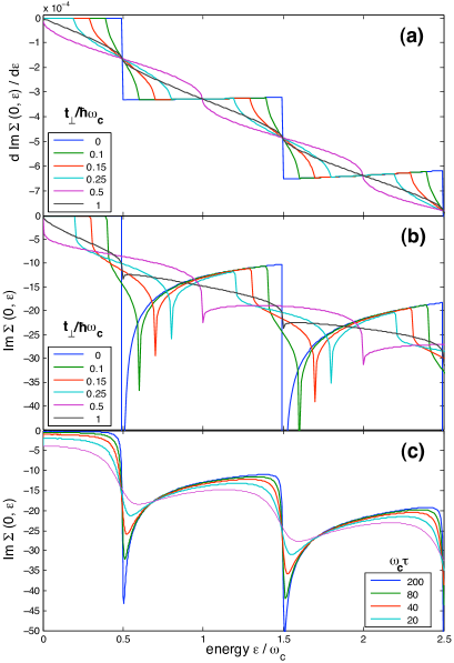
Figure 1: The imaginary part ${\mathcal{I}m}\Sigma(\epsilon)$ of the self-energy, as a function of $t_{\perp}/\hbar\omega_{c}$, at $T=0$. (a) shows ${\mathcal{I}m}\partial\Sigma/\partial\epsilon$ for the spin fluctuation model; we fix $g_{q}=g=0.58$ eV, $\chi_{0}=80$ states/eV, $\xi=2.5a$ and $\omega_{SF}=10$ meV. (b) shows ${\mathcal{I}}m\Sigma$ (with no derivative) for the non-Fermi liquid model, assuming $s=3$; we fix $K_{s=3}=0.013(\hbar\omega_{c})^{2/3}\mu^{1/3}$ with $\mu=6000~{}K$. (c) shows the effect of impurity scattering on the NFL model; we plot ${\mathcal{I}m}\Sigma(\epsilon)$ for different values of $\omega_{c}\tau$, assuming $t_{\perp}/\hbar\omega_{c}=0.75$.

In a finite field, $\Sigma(\omega)$ can be evaluated analytically, but the expression is extremely lengthy Sigrs . The essential result is shown in Fig. 1; Landau quantization introduces a “step-like” behaviour in $\partial{\mathcal{I}m}\Sigma/\partial{\epsilon}$, with corresponding singularities in ${\mathcal{R}e}\Sigma(\epsilon)$, at $\epsilon=\epsilon_{\nu}$. Notice how rapidly this singular behaviour is suppressed by interplane hopping – it is almost invisible once $t_{\perp}\sim\hbar\omega_{c}$. Impurity scattering has a similar effect (not shown in Fig. 1).

Model (b) Non-Fermi liquid model: We now couple the band electrons to fluctuations with propagator gauge :

$$\chi({\bf q},\omega)={q\over\chi q^{s}-i\gamma\omega}$$ (5)

where $s$ is a dynamic scaling exponent, with $2\leq s\leq 3$, using a fermion fluctuation coupling $g_{q}=K_{s}$. The zero field self-energy has the NFL forms $\Sigma(\epsilon)\sim\epsilon\ln\epsilon$ (for $s=2$) and $\Sigma(\epsilon)\sim(i\Omega_{0}/\epsilon)^{1\over 3}\epsilon$ (for $s=3$), so that $z_{\bf k}(\epsilon)\to 0$ on the Fermi surface. In a finite field, $\Sigma_{\nu}(k_{z},z)$ can again be evaluated analytically in the form (2), with the coefficients $\Sigma_{r}(z)$ taking the interesting $T=0$ form :

$$\Sigma_{r}(z)\;=\; {sK_{s}\over 2r^{2/s}}\left[{\cal Z}_{r}^{1\over 2}S_{2}\left({1\over 2}+{2\over s},{1\over 2};{\cal Z}_{r}\right)-{\cal Z}_{r}^{2/s}\right.$$ (6)

$$-\;\left.(-{\cal Z}_{r})^{1\over 2}S_{2}\left({1\over 2}+{2\over s},{1\over 2};-{\cal Z}_{r}\right)+(-{\cal Z}_{r})^{2/s}\right]$$

(and a more complicated finite $T$ form), where $S_{2}$ is a Lommel function Lommel , and ${\cal Z}_{r}=2\pi rz/\hbar\omega_{c}$. Now the singular behaviour in $\Sigma$ is far more pronounced; again, it is eliminated by switching on $t_{\perp}$ (Fig. 1(b)), or by impurity scattering (calculated in Fig. 1(c) in a self-consistent Born approximation).

We see that both models show singular behaviour of $\Sigma(\epsilon)$ as a function of $\epsilon$, implying similar behaviour for the quasiparticle weight $z_{k}(\epsilon)$. At the Fermi energy, $\Sigma(\epsilon=\mu)$ will then show the same singular behaviour as a function of $B$, periodic in $1/B$. Strictly speaking, this means a breakdown of FL theory for both models, but much more strongly for the NFL system. Because these singularities are rapidly suppressed by both inter-plane hopping and impurity scattering, this breakdown will only be clearly visible when $t_{\perp},\hbar/\tau\ll\hbar\omega_{c}$.

(ii) Thermodynamic potential $\Omega$: If “crossed graphs” can be ignored in $\Sigma(z)$, we can write an expression for $\Omega$ in terms of ${\cal G}$ CS :

$$\Omega=-{1\over\beta}{\mathrm{T}r}\ln\left[\left(\bar{\mathcal{G}}+{\mathcal{G}}_{osc}\right)^{-1}\right]$$ (7)

where $\bar{\mathcal{G}}$ is the non-oscillatory part of ${\mathcal{G}}$. This expression resembles the classic Luttinger/ES expression ES for $\Omega$, except that the latter drops ${\mathcal{G}}_{osc}$ from (7). This is justified in 3d, but not in 2d CS ; in the quasi-2d case it is only justified if $t_{\perp}\gg\hbar\omega_{c}$. From (7) we find $\Omega=\bar{\Omega}+2\sum_{r=1}^{\infty}(-1)^{r}\Omega_{r}\cos(r\hbar A_{F}/eB)$, where $\bar{\Omega}$ is the non-oscillatory part of $\Omega$, and

$$\Omega_{r}=\;- {m\over\hbar^{2}\beta}\sum_{n>0}\;[J_{o}^{2}\left({4\pi rt_{\perp}\over\hbar\omega_{c}}\right)\zeta_{r}(\omega_{n})$$ (8)

$$-\;{\hbar\omega_{c}\over 2\pi r}J_{o}\left({4\pi rt_{\perp}\over\hbar\omega_{c}}\right)\exp(-{2\pi r\over\hbar\omega_{c}}(\omega_{n}+\zeta(\omega_{n}))]$$

where the $\zeta_{r}(\omega_{n})=i\Sigma_{r}(i\omega_{n})$ are real and positive. Equation (8) reduces to the Luttinger/ES expression for $\Omega$ if we drop the first term, and if in the second term we use only the non-oscillatory part $\bar{\zeta}(\omega_{n})$ of $\zeta(\omega_{n})=i\Sigma(i\omega_{n})$. It further reduces to LK if we assume $\Sigma(\omega)\rightarrow(1-m/m^{*})\omega+i/2\tau$, ie., a mass renormalisation and scattering rate both independent of energy. Clearly (Fig. 1) the oscillatory part of $\Sigma$ must not in general be neglected.

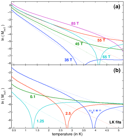
Figure 2: $\ln{M_{r}}$ for $r=1$ against $T$ (the “mass plot”), for the spin fluctuation model: (a) Plot for different fields, assuming $t_{\perp}=15K$ but no impurity scattering (when $B=55~{}T$, $\hbar\omega_{c}=20~{}K$); (b) Plot for different impurity scattering rates, assuming $t_{\perp}/\hbar\omega_{c}=0.6$. The dashed lines are fits to LK.

(iii) Oscillatory Magnetisation: We write the magnetisation at constant chemical potential $M_{\mu}(B)=-\left.\partial\Omega/\partial B\right|_{\mu}$ in the form $M=\bar{M}(B)+2\sum_{r}(-1)^{r}M_{r}$, where $\bar{M}$ is the non-oscillatory part ($M(B)$ at constant $N$ is found by making a Legendre transform Legendre ). Differentiating (8), we get $M_{r}=M_{1}^{r}+M_{2}^{r}$, with

$$M_{1}^{r}\;=\; -\Omega_{r}\sin(r\hbar A_{F}/eB)$$ (9)

$$M_{2}^{r}\;=\; -{\partial\Omega_{r}\over\partial B}\cos(r\hbar A_{F}/eB)$$

The key point here is that if $\Sigma$ contains strong oscillations with energy, these translate into a very strong new oscillatory contribution to $M_{osc}$.

Equation (9) yields a very rich variety of forms for $M(B)$, depending on the two parameters $t_{\perp}/\hbar\omega_{c}$, $\omega_{c}\tau$, and on the form and strength of the interactions. We have no space here to discuss the whole parameter range, but we can summarize the key features:

Figure 3: The dHvA component $M_{r}$ for $r=1$, against $1/B$ (again, if $B=55~{}T$, $\hbar\omega_{c}=20~{}K$), for different values of $t_{\perp}$ (measured in $K$), with no impurity scattering; we assume $T=1~{}K$. (a) for the spin fluctuation model; and (b) for the non-Fermi liquid model with $s=3$ (the topmost curve in (b) has been rescaled by a factor $0.5$).

1. Clear departures are seen from LK theory, even in mass plots (Fig. 2), for NFL systems and even for FL unless the fluctuation energy scale $\omega_{SF}\gg\hbar\omega_{c}$, and/or $\omega_{c}\tau<1$. Without interactions, only the 2nd term ($\propto J_{0}$) survives in (8); this term is well-known in LK theory J0 . With interactions, the two terms compete – as the field-induced singularities in $\Sigma(\epsilon)$ (and hence in $\zeta(\omega_{n})$ become stronger, the 1st term in $\Omega_{r}$ ($\propto J_{0}^{2}$) increases, and for NFL it can dominate the 2nd term. The much stronger singular structure in $\Sigma(\epsilon)$ means that NFL have much stronger departures from LK than FL.

2. The form of $M(B)$ depends strongly on $t_{\perp}/\hbar\omega_{c}$. This gives a remarkable structure in field plots (Fig. 3), which is eliminated by strong impurity scattering (Fig. 2(b)), or by removing strong correlation effects.

3. Short-range impurity scattering strongly suppresses the singular structure from interactions once $\omega_{c}\tau<1$ (see Fig. 2(b)). However, curiously, it affects $M_{1}^{r}$ and $M_{2}^{r}$ rather differently; $M_{1}^{r}$ decreases exponentially with $1/\omega_{c}\tau$ (à la Dingle) but $M_{2}^{r}$ decreases approximately as a power law. More refined analysis of the effect of scattering off impurities and off small angle scatterers (like dislocations) is certainly necessary for this problem.

We see that interactions have profound effects on the quasiparticles and the thermodynamics of conducting systems in high fields, for quasi-2d systems. These effects are rapidly removed by interplane coupling (once $t_{\perp}>\hbar\omega_{c}$), and even more rapidly by impurity scattering (once $\omega_{c}\tau<1$). The models we have used are of course rather simple (although very widely used in the literature); but our main results are not crucially changed by, eg., adding vertex corrections.

Consider now the experimental situation. Experiments on YBCO fall precisely in the crossover regime, with $t_{\perp}\sim 15$ K, and 15 K $\lesssim\hbar\omega_{c}\lesssim 30$ K. It is not yet possible to compare the experimental fits ybco on YBCO and Tl-2201 with the theory here, because these fits have not included the $J_{0}$ term (which already exists in LK theory J0 ). It will be extremely interesting to have fits to different strong-correlation models – and to discriminate between FL and NFL models. We note that absence of the $J_{0}^{2}$ term in (8) would indicate the underlying state is FL (but NFL if the $J_{0}^{2}$ term is strong). It will also be interesting to look more closely at other strongly-correlated quasi-2d systems in high fields – where few departures from LK have been found so far. Finally, note that any experiments sensitive to the singular structure we find in ${\cal G}$ should show interesting effects. Obvious examples are c-axis tunneling and SdH experiments in very high fields, but a generalisation of the foregoing to a transport theory will be required.

This work was supported by NSERC, CIFAR and PITP. We thank P. W. Anderson, D. Bonn, S. Julian, B. Ramshaw, and G. A. Sawatzky for discussions.

References

- (1) I. M. Lifshitz and A. M. Kosevich, Sov. Phys. JETP 2, 646 (1956); D. Shoenberg, Magnetic Oscillations in Metals (Cambridge Univ. Press, 1984). We ignore “spin factors” in this paper.
- (2) J. M. Luttinger, Phys. Rev. 121, 1251 (1961); Y. Bych’kov, L. P. Gor’kov, Sov. Phys. JETP 14, 1132 (1962)
- (3) M. Fowler, R. E. Prange, Physica 1, 315 (1965); S. Engelsberg, G. Simpson, Phys. Rev. B 2, 1657 (1970); A. Wasserman, M. Springford, Adv. Phys. 45, 471 (1996).
- (4) See, eg., M. Elliot, T. Ellis, M. Springford, J. Phys. F10, 2681 (1980); or A. McCollum et. al., Physica B403, 717 (2008), and refs. therein.
- (5) See, eg., The Quantum Hall effect, ed. R.E. Prange, S.M. Girvin (Springer-Verlag, 1990).
- (6) For YBCO, see C. Jaudet et al., Phys. Rev. Lett. 100, 187005 (2008); A. Audouard et al., /condmat 0812.0458; for the system, see B. Vignolle et al., Nature 455, 952 (2008)
- (7) C. Bergemann et al., Adv. Phys. 52, 639 (2003); F. Bauemberger et al., Phys. Rev. Lett. 96, 246402 (2006)
- (8) J. Wosnitza et al., New J. Phys. 10, 083032 (2008).
- (9) A. Shekhter, A. M. Finkelstein, Proc. Nat. Acad. Sci. 103, 15765 (2006).
- (10) For exact 2d results for large Landau levels, see R. Moessner, J.T. Chalker, Phys. Rev. B54, 5006 (1996).
- (11) Such “nearly antiferromagnetic spin fluctuation” models for conducting systems go back to T. Moriya, Phys. Rev. Lett. 24, 1433 (1970). They have been applied by many authors to high- systems; early papers are T. Moriya et al., J. Phys. Soc. Jap. 59, 2905 (1990), and A.J. Millis, P. Monthoux, D. Pines, Phys. Rev. B42, 167 (1990).
- (12) Vertex corrections to eqn (1) change the numerical results, but not the basic form of , or of the dHvA oscillations, for the spin fluctuation model.
- (13) The self-energy , and the coefficients , can be found analytically for the spin fluctuation model as a a rather cumbersome function of elliptic integrals and exponential integrals.
- (14) Models in which fermions couple to fluctuation propagators of form (5) have been studied extensively in high- systems and for the FQHL; see, eg., P.A. Lee., N. Nagaosa, Phys. Rev. B46, 5621 (1992), and B.I. Halperin, P.A. Lee, N. Read, Phys. Rev. B47, 7312 (1993). The importance of vertex corrections to this model depends on how it is formulated. In a expansion, vertex corrections can be neglected for large ; see J. Polchinski, Nucl. Phys B422, 617 (1994).
- (15) For Lommel functions, see G.N. Watson, A treatise on the theory of Bessel functions (Cambridge Univ Press, 1952), section 10.7. The function is also written as in the literature.
- (16) S. Curnoe and P. C. E. Stamp, Phys. Rev. Lett. 80, 3312 (1998)
- (17) It is convenient to do field-theoretical calculations at constant . To find, eg., (ie., at constant ), we calculate , with ; then .
- (18) K. Yamaji, J. Phys. Soc Jap. 58, 1520 (1989).