Implications of $D^{0}-\overline{D^{0}}$ on the rare top quark decays $t\to u\gamma$ and $t\to ug$

Abstract

The recently observed mass difference of the $D^{0}-\overline{D^{0}}$ mixing is used to predict the branching ratios of the rare top quark decays $t\to u\gamma$ and $t\to ug$ in a model independent way using the effective Lagrangian approach. It is found that $Br(t\to u\gamma)<4\times 10^{-4}$ and $Br(t\to ug)<2\times 10^{-3}$, which still may be within reach of the LHC collider.

I Introduction

With the recent start of the up–and–coming experimental program of the Large Hadron Collider (LHC) at CERN, the search for new physics effects at the TeV scale enters into an exciting era. In particular, due to the expected copious production of top quark events, clues of physics beyond the Fermi scale could be evidenced. The flavor changing neutral current (FCNC) transitions of the top quark are good processes to look for signals of new physics, since the new dynamical effects are likely more evident in those top quark processes that are forbidden or strongly suppressed in the standard model (SM) review . In the SM, the FCNC top transitions $t\to cg$, $t\to c\gamma$, $t\to cZ$, and $t\to cH$ arise at the one–loop level, being considerably GIM–suppressed, as they have branching ratios ranging from $10^{-10}$ to $10^{-13}$ DMPR ; EHS1 ; EHS2 ; MP . The decays involving in the final state the quark $u$ instead of $c$ are much more suppressed due to Kobayashi–Maskawa effects. On the other hand, the three body $t\to cgg$ EFT and $t\to c\bar{c}c$ CHTT1 ; CHTT2 transitions have also been studied within the context of the SM. It was found EFT ; CHTT1 ; CHTT2 the surprising result that the branching rations for these decays are respectively one order of magnitude larger and of the same order of magnitude when compared with the two–body $t\to cg$ decay. Beyond the SM, FCNC top quark decays have been the subject of considerable interest in the literature, as they can have branching ratios much larger than the SM ones. These type of top transitions have been studied in some extended theories such as the two–Higgs doublet model (THDM) THDM11 ; THDM12 ; THDM13 ; THDM21 ; THDM22 ; THDM23 ; THDM24 ; THDM31 ; THDM32 , supersymmetric (SUSY) models with nonuniversal soft breaking SUSY1 ; SUSY2 ; SUSY3 ; SUSY4 ; SUSY5 ; SUSY6 ; SUSY7 ; SUSY8 ; SUSY9 ; SUSY10 ; SUSY11 , SUSY models with broken R–parity SUSYR1 ; SUSYR2 , models with extra $Z^{\prime}$ gauge bosons ZP , and even more exotic scenarios ES1 ; ES2 ; ES3 ; ES4 . Similar results were obtained within the context of effective theories ETS1 ; ETS2 ; ETS3 .

In this work, we are interested in using the mass difference $\Delta M_{D}$ in the $D^{0}-\overline{D^{0}}$ mixing recently observed by the Babar Babar and Belle Belle collaborations to impose a bound on the branching ratios for the FCNC top quark $t\to u\gamma$ and $t\to ug$ decays. It turns out that due to electromagnetic gauge invariance, the $t\to u\gamma$ transition is somewhat restricted, as it can occurs only through two electromagnetic gauge structures of dipolar type, which are characterized by Lorentz tensor structures of the form $\sigma_{\mu\nu}q^{\nu}$ (transition magnetic dipole moment), with $q_{\mu}$ the photon momentum, or $\gamma_{5}\sigma_{\mu\nu}q^{\nu}$ (transition electric dipole moment). The $t\to ug$ decay occurs through the analogous chromomagnetic and chromoelectric dipole moments. These interactions are naturally suppressed, as they can arise in renormalizable theories only through quantum fluctuations of one–loop or higher orders.

An outline of this paper is as follows. In section II we briefly study the couplings arising from the effective Lagrangian. Section III is devoted to obtain the leading contribution of the $tu_{i}\gamma$ and $tu_{i}g$ couplings to the mass difference $\Delta M_{D}$ of the $D^{0}-\overline{D^{0}}$ mixing. Finally, in section IV we comment our results.

II Effective Lagrangian for the $tu_{i}\gamma$ and $tu_{i}g$ couplings

The most general structure for the $tu\gamma$ and $tug$ couplings arise from the following dimension–six $SU_{C}(3)\times SU(2)_{L}\times U_{Y}(1)$–invariant effective Lagrangian:

$${\cal L}^{Up-FCNC}_{eff} = \frac{\alpha^{ij}_{uB}}{\Lambda^{2}}(\bar{Q}_{i}\sigma_{\mu\nu}B^{\mu\nu}u_{j}\tilde{\Phi})+\frac{\alpha^{ij}_{uW}}{\Lambda^{2}}(\bar{Q}_{i}\sigma_{\mu\nu}W^{\mu\nu}u_{j}\tilde{\Phi})$$ (1)

$$+ \frac{\alpha^{ij}_{uG}}{\Lambda^{2}}(\bar{Q}_{i}\sigma_{\mu\nu}G^{\mu\nu}u_{j}\tilde{\Phi}),$$

where $Q^{\prime}$ and $u^{\prime}$ stand for left– and right–handed doublet and singlet of $SU_{L}(2)$, respectively and a sum over quark flavor is implied. Here, $B_{\mu\nu}$, $W_{\mu\nu}=\sigma^{i}W^{i}_{\mu\nu}/2$, and $G_{\mu\nu}^{a}=\lambda^{a}G_{\mu\nu}/2$ are the gauge tensors associated with the $U_{Y}(1)$, $SU_{L}(2)$, and $SU_{C}(3)$ groups, respectively. On the other hand, $\tilde{\Phi}=i\sigma^{2}\Phi^{*}$, with $\Phi$ the SM Higgs doublet. In addition, the $\alpha^{ij}$ are the coefficients of general $3\times 3$ matrices defined in the flavor space, whereas $\Lambda$ represents the new physics scale. This parametrization allow us to treat in a model–independent way FCNC transitions in the up quark sector mediated by massless gauge bosons.

After spontaneous symmetry breaking, ${\cal L}^{Up-FCNC}_{eff}$ can be diagonalized as usual via the $V^{u}_{L}$ and $V^{u}_{R}$ unitary matrices, which relate gauge states to mass eigenstates. In particular, the $u_{i}u_{j}\gamma$ and $u_{i}u_{j}g$ vertices are given by the following Lagrangian:

$${\cal L}_{\overline{U}U\gamma(g)} = \frac{g}{2\sqrt{2}m_{W}}\Big{(}\overline{U}(\omega^{\gamma}P_{R}+\omega^{\gamma{\dagger}}P_{L})\sigma_{\mu\nu}UF^{\mu\nu}$$ (2)

$$+\overline{U}(\omega^{g}P_{R}+\omega^{g{\dagger}}P_{L})\sigma_{\mu\nu}\frac{\lambda^{a}}{2}UG^{a\mu\nu}\Big{)},$$

where $\overline{U}=(\bar{u},\bar{c},\bar{t})$ are vectors in the flavor space. Notice the presence of the global factor $g/\sqrt{2}m_{W}$, which arises from the Higgs mechanism and is common to both electromagnetic and strong couplings. In the above expression, $\omega^{\gamma}$ and $\omega^{g}$ are flavor matrices given by

$$\omega^{\gamma} = \Big{(}\frac{v}{\Lambda}\Big{)}^{2}V^{u}_{L}\big{(}c_{W}\alpha_{uB}+\frac{1}{2}s_{W}\alpha_{uW}\big{)}V^{u{\dagger}}_{R},$$ (3)

$$\omega^{g} = \Big{(}\frac{v}{\Lambda}\Big{)}^{2}V^{u}_{L}\alpha_{uG}V^{u{\dagger}}_{R},$$ (4)

where $v\approx 246$ GeV is the Fermi scale and $c_{W}$ ($s_{W}$) stands for cosine (sine) of the weak angle. To generate vector–mediated FCNC effects at the tree level in the effective theory, it is assumed that the $V^{u}_{L,R}$ matrices diagonalize the Yukawa mass matrix $Y^{u}$ but not the matrices $\alpha_{uB(uW)}$ and $\alpha_{uG}$. From the above expressions, it is immediate to derive the vertex functions for the $tu_{i}\gamma$ and $tu_{i}g$ ($u_{i}=u,c$) couplings, which can be written as

$$\Gamma^{(\gamma,g)}_{\mu}(q)=\frac{g}{\sqrt{2}m_{W}}\Big{(}\kappa^{(\gamma,g)}_{tu_{i}}+i\tilde{\kappa}^{(\gamma,g)}_{tu_{i}}\gamma_{5}\Big{)}\sigma_{\mu\nu}q^{\nu}\delta^{(\gamma,g)},$$ (5)

where $\delta^{\gamma}=1$ and $\delta^{g}=\lambda^{a}/2$. In addition, $\kappa^{(\gamma,g)}_{tu_{i}}=Re(\omega^{(\gamma,g)}_{tu_{i}})$ and $\tilde{\kappa}^{(\gamma,g)}_{tu_{i}}=Im(\omega^{(\gamma,g)}_{tu_{i}})$. As we will see below, it is not possible to isolate the contribution of the $tuV$ and $tcV$ ($V=\gamma,g$) couplings from the $D^{0}-\overline{D^{0}}$ mixing. This contribution is given through an amplitude that depends symmetrically on both vertices. Due to this, it is not possible to obtain bounds for the $t\to c\gamma$ and $t\to cg$ decays without making additional assumptions.

III $tu_{i}\gamma$ and $tu_{i}g$ contributions to $D^{0}-\overline{D^{0}}$ mixing

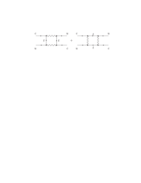
Figure 1: Simultaneous contribution of the $tc\gamma$ and $tcu$ couplings to the $D^{0}-\overline{D^{0}}$ mixing. The contribution of the $tcg$ and $tug$ couplings also is given through this type of diagrams.

We now are in position of deriving the contribution of the $tu_{i}\gamma$ and $tu_{i}g$ vertices to the mass difference $\Delta M_{D}$ of the $D^{0}-\overline{D^{0}}$ mixing. These contributions occur through short distance effects characterized by the box diagrams shown in FIG.1. Neglecting the external momenta, the $tu_{i}\gamma$ and $tu_{i}g$ couplings generate an amplitude given by:

$$T = 2\Bigg{(}\frac{g}{\sqrt{2}m_{W}}\Bigg{)}^{4}\Bigg{(}|\omega^{\gamma}_{tu}|^{2}|\omega^{\gamma}_{tc}|^{2}+\frac{11}{18}|\omega^{g}_{tu}|^{2}|\omega^{g}_{tc}|^{2}\Bigg{)}$$ (6)

$$\times\int\frac{d^{D}k}{(2\pi)^{D}}\frac{(\bar{u}_{L}\sigma_{\mu\lambda}k^{\lambda}\hbox{\large$/$}\kern-5.76042pt\hbox{$k$}\sigma_{\alpha\rho}k^{\rho}c_{L})(\bar{u}_{L}\sigma_{\mu\eta}k^{\eta}\hbox{\large$/$}\kern-5.76042pt\hbox{$k$}\sigma_{\mu\xi}k^{\xi}c_{L})}{(k^{2})^{2}(k^{2}-m^{2}_{t})^{2}}.$$

The integral involved in (6) is of the form

$$I^{(a,b)}_{\alpha\beta\mu\nu\lambda\rho}\equiv\int\frac{d^{D}k}{\left(2\pi\right)^{D}}\frac{k_{\alpha}k_{\beta}k_{\mu}k_{\nu}k_{\lambda}k_{\rho}}{(k^{2})^{a}(k^{2}-m^{2}_{t})^{b}},$$

with $a=2$ and $b=2$, and it diverges quadratically at $D=4$. As discussed in reference BL , the use of cutoffs to regularize quadratic or higher divergent integrals would violate the decoupling theorem, as this scheme introduce a strong dependence on the new physics scale. In our case, the use of a cutoff leads to an amplitude proportional to $\Lambda^{2}$, which would overestimate our prediction. Only a logarithmic dependence on the new physics scale is physically acceptable BL ; W (for some applications of dimensional regularization in effective Lagrangians see, for instance, Refs. Tosca1 ; Tosca2 ; Tosca3 ). Thus, we do not use a cutoff to regularize our amplitude, instead we will use dimensional regularization, which allow one to convert the quadratic divergence into a logarithmic one through the following limit delbourgo-scadron1 ; delbourgo-scadron2 :

$$\lim_{\varepsilon\to 0}\left(I^{(2,2)}_{\alpha\beta\mu\nu\lambda\rho}-2m^{2}_{t}I^{(2,3)}_{\alpha\beta\mu\nu\lambda\rho}\right) = -\frac{im^{2}_{t}}{3072\pi^{2}}\bigg{[}g_{\alpha\beta}\left(g_{\mu\nu}g_{\lambda\rho}+g_{\mu\lambda}g_{\nu\rho}+g_{\nu\lambda}g_{\mu\rho}\right)$$ (7)

$$+g_{\alpha\mu}\left(g_{\beta\nu}g_{\lambda\rho}+g_{\beta\lambda}g_{\nu\rho}+g_{\beta\rho}g_{\nu\lambda}\right)$$

$$+g_{\alpha\nu}\left(g_{\beta\mu}g_{\lambda\rho}+g_{\beta\lambda}g_{\mu\rho}+g_{\beta\rho}g_{\nu\lambda}\right)$$

$$+g_{\alpha\lambda}\left(g_{\beta\rho}g_{\mu\nu}+g_{\beta\nu}g_{\mu\rho}+g_{\beta\mu}g_{\nu\rho}\right)$$

$$+g_{\alpha\rho}\left(g_{\beta\lambda}g_{\mu\nu}+g_{\beta\mu}g_{\nu\lambda}+g_{\beta\nu}g_{\mu\lambda}\right)\bigg{]}.$$

The arising integral with logarithmic divergence, $I^{(2,3)}_{\alpha\beta\mu\nu\lambda\rho}$, can be treated in the usual manner, hence a renormalization scheme can directly be applied to the amplitude in (6).

Once the integral is solved, one obtains the result for the amplitude:

$$T = -\frac{i\alpha^{2}}{s^{4}_{W}m^{2}_{W}}\Big{(}\frac{21}{4}\Big{)}\Big{(}\frac{m_{t}}{m_{W}}\Big{)}^{2}\Bigg{(}|\omega^{\gamma}_{tu}|^{2}|\omega^{\gamma}_{tc}|^{2}+\frac{11}{18}|\omega^{g}_{tu}|^{2}|\omega^{g}_{tc}|^{2}\Bigg{)}$$ (8)

$$\times(\bar{u}_{L}\gamma_{\mu}c_{L})(\bar{u}_{L}\gamma^{\mu}c_{L})\Bigg{(}\Delta+\log\Big{(}\ \frac{\mu^{2}}{m^{2}_{t}}\Big{)}+\frac{19}{12}\Bigg{)},$$

where the ultraviolet divergence is contained in $\Delta=\frac{2}{\varepsilon}-\gamma_{E}+\log(4\pi)$, with $\varepsilon=4-D$ and $\gamma_{E}$ the Euler’s constant. Here, $\mu$ is the dimensional regularization scale. Following Refs.BL ; W ; Tosca1 ; Tosca2 ; Tosca3 ; RMS1 ; RMS2 , the divergent term in this amplitude can be absorbed by renormalizing the appropriated coefficients of the complete effective Lagrangian since it already contains all the invariants allowed by the SM symmetry. The invariants needed to absorb the divergences are of the form $(\alpha_{12}/\Lambda^{2})(\bar{q}_{1}\gamma_{\mu}q_{2})(\bar{q}_{1}\gamma^{\mu}q_{2})$, with $\bar{q}_{1}=(\bar{u}_{L},\bar{d}_{L})$ and $\bar{q}_{2}=(\bar{c}_{L},\bar{s}_{L})$, etc. Using the $\overline{MS}$ renormalization scheme with $\mu=\Lambda$, the renormalized amplitude can be written as follows:

$$T = -\frac{i\alpha^{2}}{s^{4}_{W}m^{2}_{W}}\Big{(}\frac{21}{4}\Big{)}\Big{(}\frac{m_{t}}{m_{W}}\Big{)}^{2}\Bigg{(}|\omega^{\gamma}_{tu}|^{2}|\omega^{\gamma}_{tc}|^{2}+\frac{11}{18}|\omega^{g}_{tu}|^{2}|\omega^{g}_{tc}|^{2}\Bigg{)}$$ (9)

$$\qquad\times(\bar{u}_{L}\gamma_{\mu}c_{L})(\bar{u}_{L}\gamma^{\mu}c_{L})f(\Lambda/m_{t}),$$

where we have defined the dimensionless function $f(\Lambda/m_{t})=\log\Big{(}\frac{\Lambda^{2}}{m^{2}_{t}}\Big{)}+\frac{19}{12}$. It is easy to see that this amplitude can be obtained directly from a four–quark effective interaction

$${\cal L}_{eff}=-\frac{\alpha^{2}}{s^{4}_{W}m^{2}_{W}}\Big{(}\frac{21}{16}\Big{)}\Big{(}\frac{m_{t}}{m_{W}}\Big{)}^{2}\Bigg{(}|\omega^{\gamma}_{tu}|^{2}|\omega^{\gamma}_{tc}|^{2}+\frac{11}{18}|\omega^{g}_{tu}|^{2}|\omega^{g}_{tc}|^{2}\Bigg{)}f(\Lambda/m_{t})Q_{1},$$ (10)

where the dimension–six operator $Q_{1}=(\bar{u}_{L}\gamma_{\mu}c_{L})(\bar{u}_{L}\gamma^{\mu}c_{L})$ is well known in the literature Operators . In the above expression, a factor of $1/4$ was introduced in order to compensate the $(2!)(2!)$ Wick contractions.

On the other hand, the mass difference $D$ is given by

$$\Delta M_{D}=\frac{1}{M_{D}}Re<\overline{D^{0}}|{\cal H}_{eff}=-{\cal L}_{eff}|D^{0}>,$$ (11)

which in our case takes the form

$$\Delta M_{D} = \frac{\alpha^{2}}{s^{4}_{W}m^{2}_{W}}\Big{(}\frac{21}{16}\Big{)}\Big{(}\frac{m_{t}}{m_{W}}\Big{)}^{2}\Bigg{(}|\omega^{\gamma}_{tu}|^{2}|\omega^{\gamma}_{tc}|^{2}+\frac{11}{18}|\omega^{g}_{tu}|^{2}|\omega^{g}_{tc}|^{2}\Bigg{)}f(\Lambda/m_{t})<Q_{1}>$$

$$= \Big{(}\frac{21}{24}\Big{)}\frac{\alpha^{2}}{s^{4}_{W}}\Big{(}\frac{m_{t}}{m_{W}}\Big{)}^{2}\Big{(}\frac{f_{D}}{m_{W}}\Big{)}^{2}M_{D}\Bigg{(}|\omega^{\gamma}_{tu}|^{2}|\omega^{\gamma}_{tc}|^{2}+\frac{11}{18}|\omega^{g}_{tu}|^{2}|\omega^{g}_{tc}|^{2}\Bigg{)}f(\Lambda/m_{t})B_{1},$$

where the expressions for $<Q_{1}>$ given in Ref.Operators were used. Here, $f_{D}$ is the $D$ decay constant. We will use the CLEO Collaboration determination $f_{D}=222.6\pm 16.7MeV$ CLEO . The factor $B_{1}$ is unknown, but lattice calculation Lattice leads to $B_{1}\approx 0.8$, although in vacuum saturation and in the heavy quark limit it approximates to the unity. In our numerical analysis, we will use $B_{1}=1$. Using the value $M_{D}=1.8646$ GeV, one obtains

$$\Delta M_{D}=6.28\times 10^{-8}f(\Lambda/m_{t})\Bigg{(}|\omega^{\gamma}_{tu}|^{2}|\omega^{\gamma}_{tc}|^{2}+\frac{11}{18}|\omega^{g}_{tu}|^{2}|\omega^{g}_{tc}|^{2}\Bigg{)}.$$ (13)

From the experimental side, the Heavy Flavor Averaging Group HFAG interpretation of the current data leads to a mass difference of $D^{0}-\overline{D^{0}}$ given by $\Delta M_{D}=(1.4\pm 0.5)\times 10^{-15}$ GeV PDG . To bound the $\kappa_{i}$ coefficients, we demand that the above contribution does not exceed the experimental uncertainty, which leads to

$$|\omega^{\gamma}_{tu}|^{2}|\omega^{\gamma}_{tc}|^{2}+\frac{11}{18}|\omega^{g}_{tu}|^{2}|\omega^{g}_{tc}|<7.96\times 10^{-9},$$ (14)

where it was assumed that $f(\Lambda/m_{t})\sim O(1)$. This assumption is reasonable MQ , as a new physics scale in the TeVs region is expected. Considering the electromagnetic and strong contributions one at the time, one obtains

$$|\omega^{\gamma}_{tu}||\omega^{\gamma}_{tc}| < 8.92\times 10^{-5},$$ (15)

$$|\omega^{g}_{tu}||\omega^{g}_{tc}| < 1.14\times 10^{-4}.$$ (16)

From general considerations, one can expect that $\omega^{\gamma,g}_{tc}>\omega^{\gamma,g}_{tu}$, so that a conservative point of view allow us to obtain the bounds

$$|\omega^{\gamma}_{tu}|^{2} < 8.92\times 10^{-5},$$ (17)

$$|\omega^{g}_{tu}|^{2} < 1.14\times 10^{-4}.$$ (18)

It should be noticed that it is not possible to bound the $tc\gamma$ and $tcg$ without making additional assumptions.

On the other hand, the branching ratios for the $t\to u\gamma$ and $t\to ug$ decays are given by

$$Br(t\to u\gamma) = \frac{\alpha}{4s^{2}_{W}}\Big{(}\frac{m_{t}}{\Gamma_{t}}\Big{)}\Big{(}\frac{m_{t}}{m_{W}}\Big{)}^{2}|\omega^{\gamma}_{tu}|^{2},$$ (19)

$$Br(t\to ug) = \frac{\alpha}{s^{2}_{W}}\Big{(}\frac{m_{t}}{\Gamma_{t}}\Big{)}\Big{(}\frac{m_{t}}{m_{W}}\Big{)}^{2}|\omega^{g}_{tu}|^{2}.$$ (20)

From these expressions and from Eqs.(15,16), we obtain the following bounds for these decays

$$Br(t\to u\gamma) < 3.9\times 10^{-4},$$ (21)

$$Br(t\to ug) < 2.02\times 10^{-3},$$ (22)

where the approximation $\Gamma_{t}\approx\Gamma(t\to bW)=1.55$ GeV for the total top decay width was used.

It is worth comparing our results with those predictions obtained in some specific models. Most of the known results are on the $t\to c\gamma$ and $t\to cg$ decays, which are strongly suppressed in the SM, with branching ratios of order of $10^{-13}$ and $10^{-11}$ EHS1 ; EHS2 , respectively. The branching ratios for the decays involving the quark $u$ instead of $c$ are even more suppressed by a Kobayashi–Maskawa factor of $(V_{ub}/V_{cb})^{2}\approx 10^{-2}$. Beyond the SM, these branching ratios are considerably enhanced. For instance, in the THDM-III, the $t\to c\gamma$ and $t\to cg$ decays can have a branching ratio in the range $10^{-7}-10^{-12}$ and $10^{-4}-10^{-8}$ THDM21 ; THDM22 ; THDM23 ; THDM24 , respectively. On the other hand, the respective predictions in some SUSY models SUSY1 ; SUSY2 ; SUSY3 ; SUSY4 ; SUSY5 ; SUSY6 ; SUSY7 ; SUSY8 ; SUSY9 ; SUSY10 ; SUSY11 are of order of $10^{-5}$ and $10^{-3}$. An effective Lagrangian analysis of Higgs–mediated FCNC leads to branching ratios for these decays of order of $10^{-7}$ and $10^{-6}$ ZP . All these predictions are consistent with our bound, as it is expected that the branching ratios for the $t\to u\gamma$ and $t\to ug$ decays are lower by two or higher orders of magnitude than those involving the quark $c$.

IV Final remarks

To conclude, we would like to comment on the possible detection of the $t\to u\gamma$ and $t\to ug$ decays at the LHC. On the light of our bounds for their branching ratios, one can conclude that they are within reach of this collider, given the important production of $t\bar{t}$ events of several millions per year. In a purely statistical basis those channels with branching ratios larger than about $10^{-6}$ do have the chance of being detected. However, the observability of a particular channel decay depends on several factors, background and systematics may reduce this value by several orders of magnitude depending of the particular signature. For instance, the $t\to ug$ decay would require a large branching in order to be detected as it is swamped by hadronic backgrounds. However, the important difference of about three orders of magnitude between the observability parameter and our bound makes quite possible the observation of this channel. As far as the $t\to u\gamma$ mode is concerned, it could be detected even with a relatively small branching ratio because it would be produced in a cleaner environment. In conclusion, our analysis suggests that the recent observation of $D^{0}-\overline{D^{0}}$ mixing does not exclude the possibility of observing the rare top quark decays $t\to u\gamma$ and $t\to ug$ at the LHC. Since the $tc\gamma$ and $tcg$ couplings are not directly constrained by this experimental result, their observation at the LHC would be more probable.

References

• (1) For a review on top quark physics, see D. Chakraborty, J. Kongsberg, and D. Rainwater, Annu. Rev. Nucl. Part. Sci. 53, 301 (2003).
• (2) J. L. Díaz–Cruz, R. Martínez, M. A. Pérez, and A. Rosado, Phys. Rev. D41, 891 (1990).
• (3) G. Eilam, J. L. Hewett, and A. Soni, Phys. Rev. D44, 1473 (1991).
• (4) G. Eilam, J. L. Hewett, and A. Soni, Phys. Rev. D59, 039901(E) (1999).
• (5) B. Mele and S. Petrarca, Phys. Lett. B435, 401 (1998).
• (6) G. Eilam, M. Frank, and I. Turan, Phys. Rev. D73, 053011 (2006).
• (7) A. Cordero–Cid, J. M. Hernández, G. Tavares–Velasco, and J. J. Toscano, Phys. Rev. D73, 094005 (2006).
• (8) N. G. Deshpande, B. Margolis, and H. D. Trottier, Phys. Rev. D45, 178 (1992).
• (9) M. E. Luke and M. J. Savage, Phys. Lett. B307, 387 (1993).
• (10) D. Atwood, L. Reina, And A. Soni, Phys. Rev. D53, 1199 (1996).
• (11) D. Atwood, L. Reina, And A. Soni, Phys. Rev. Lett. 75, 3800 (1995).
• (12) E. O. Iltan, Phys. Rev. D65, 075017 (2002).
• (13) E. O. Iltan and I. Turan, Phys. Rev. D67, 015004 (2003).
• (14) W. S. Hou, Phys. Lett. B296, 179 (1992).
• (15) D. Atwood, L. Reina, and A. Soni, Phys. Rev. D55, 3156 (1997).
• (16) J. L. Díaz–Cruz, M. A. Pérez, G. Tavares–Velasco, and J. J. Toscano, Phys. Rev. D60, 115014 (1999).
• (17) I. Baum, G. Eilam, and S. Bar–Shalom, Phys. Rev. D77, 113008 (2008).
• (18) G. M. de Divitiis, R. Petronzio, and L. Silvestrini, Nucl. Phys. B504, 45 (1997).
• (19) J. L. Lopez, D. V. Nanopoulos, and R. Rangarajan, Phys. Rev. D56, 3100 (1997).
• (20) C. S. Li, R. J. Oakez, and J. M. Yang, Phys. Rev. D49, 293 (1994).
• (21) J. Yang and C. S. Li, Phys. Rev. D49, 3412 (1994).
• (22) G. Couture, C. Hamzaoui, and H. Konig, Phys. Rev. D52, 1713 (1995).
• (23) G. Couture, M. Frank, and H. Konig, Phys. Rev. D56, 4213 (1997).
• (24) J. Guasch and J. Sola, Nucl. Phys. B562, 3 (1999).
• (25) Jun–jie Cao, Zhao–hua Xiong, and Jin Min Yang, Nucl. Phys. B651, 87 (2003).
• (26) Jian Jun Liu, Chong Sheng Li, Li Lin Yang, and Li Gang Jin, Phys. Lett. B599, 92 (2004).
• (27) J. J. Cao, G. Eilam, Ken–ichi Hikasa, and Jin Min Yang, Phys. Rev. D74, 031701 (2006).
• (28) J. J. Cao, G. Eilam, M. Frank, K. Hikasa, G. L. Liu, I. Turan, and J. M. Yang, Phys. Rev. D75, 075021 (2007).
• (29) J. M. Yang, B.-L. Young, and X. Zhang, Phys. Rev. D58, 055001 (1998).
• (30) G. Eilam, A. Gemintern, T. Han, J. M. Yang, and X. Zhang, Phys. Lett. B510, 227 (2001).
• (31) A. Coredero–Cid, G. Tavares–Velasco, and J. J. Toscano, Phys. Rev. D72, 057701 (2005).
• (32) Chong–xing Yue, Gong–ru Lu, Quing–jun Xu, Guo–li Liu, and Guang–ping Gao, Phys. Lett. B508, 290 (2001).
• (33) J. A. Aguilar–Saavedra and B. M. Nobre, Phys. Lett. B553, 251 (2003).
• (34) Gong–ru Lu, Fu–rong Yin, Xue–lei Wang, and Ling–de Wan, Phys. Rev. D68, 015002 (2003).
• (35) R. Gaitán, O. G. Miranda, and L. G. Cabral–Rosetti, Phys. Rev. D72, 034018 (2005).
• (36) F. del Aguila, M. Pérez–Victoria, and J. Santiago, Phys. Lett. B492, 98 (2000).
• (37) F. del Aguila, M. Pérez–Victoria, and J. Santiago, J.H.E.P. 09, 011 (2000).
• (38) Adriana Cordero–Cid, M. A. Pérez, G. Tavares–Velasco, and J. J. Toscano, Phys. Rev. D70, 074003 (2004).
• (39) B. Aubert et al. (BaBar Collaboration), Phys. Rev. Lett. 98,211802 (2007).
• (40) M. Staric et al. (Belle Collaboration), Phys. Rev. Lett. 98, 211803 (2007).
• (41) C. P. Burgess and D. London, Phys. Rev. Lett. 69, 3428 (1992).
• (42) J. Wudka, Int. J. Mod. Phys. A9, 2301 (1994).
• (43) M. A. Pérez and J. J. Toscano, Phys. Lett. B289, 381 (1992).
• (44) M. A. Pérez, J. J. Toscano, and J. Wudka, Phys. Rev. D52, 494 (1995).
• (45) J. L. Díaz–Cruz, J. Hernández–Sánchez, and J. J. Toscano, Phys. Lett. B512, 339 (2001).
• (46) R. Delbourgo and M. D. Scadron, Mod. Phys. Lett. A17, 209 (2002).
• (47) R. Delbourgo and M. D. Scadron, Mod. Phys. Lett. A10, 251 (1995).
• (48) S. Weinberg, Physica A96, 327 (1979).
• (49) J.Gasser and L. Leutwyler, Nucl. Phys. B250, 465 (1985).
• (50) E. Galowich, J. Hewett, S. Pakvasa, and A. A. Petrov, Phys. Rev. D76, 095009 (2007).
• (51) M. Artuso et al. (CLEO Collaboration), Phys. Rev. Lett. 95, 251801 (2005).
• (52) R. Gupta, T. Bhattacharya, and S. R. Sharpe, Phys. Rev. D55, 4036 (1977).
• (53) Heavy Flavor Averaging Group, http://www.slac.stanford.edu/xorg/hfag/index.
• (54) W.-M. Yao et al., Journal of Physics G33, 1 (2006).
• (55) See for instance: W. J. Marciano and A. Queijeiro, Phys. Rev. D33, 3449 (1986).