Galaxy clusters identified from the SDSS DR6 and their properties

Abstract

Clusters of galaxies in most previous catalogs have redshifts $z\leq 0.3$. Using the photometric redshifts of galaxies from the Sloan Digital Sky Survey Data Release 6 (SDSS DR6), we identify 39,668 clusters in the redshift range $0.05<z<0.6$ with more than eight luminous ($M_{r}\leq-21$) member galaxies. Cluster redshifts are estimated accurately with an uncertainty less than 0.022. The contamination rate of member galaxies is found to be roughly 20%, and the completeness of member galaxy detection reaches to $\sim$90%. Monte Carlo simulations show that the cluster detection rate is more than 90% for massive ($M_{200}>2\times 10^{14}~{}M_{\odot}$) clusters of $z\leq 0.42$. The false detection rate is $\sim$5%. We obtain the richness, the summed luminosity, and the gross galaxy number within the determined radius for identified clusters. They are tightly related to the X-ray luminosity and temperature of clusters. Cluster mass is related to the richness and summed luminosity with $M_{200}\propto R^{1.90\pm 0.04}$ and $M_{200}\propto L_{r}^{1.64\pm 0.03}$, respectively. In addition, 685 new candidates of X-ray clusters are found by cross-identification of our clusters with the source list of the ROSAT X-ray survey.

1. Introduction

As the largest gravitational bound systems in the universe, clusters of galaxies are important tracers to study the large scale structure (Bahcall, 1988; Postman et al., 1992; Carlberg et al., 1996; Bahcall et al., 1997). Statistical studies of clusters constrain the cosmological parameters, for example, $\Omega_{m}$, the mass density parameter of the universe, and $\sigma_{8}$, the amplitude of mass fluctuations at a scale of 8 $h^{-1}$ Mpc (Reiprich & Böhringer, 2002; Seljak, 2002; Dahle, 2006; Pedersen & Dahle, 2007; Rines et al., 2007). The detailed studies of clusters provide the strong evidence of dark matter and constrain the abundance of dark matter in the universe (see, e.g., Ikebe et al., 1996; Castillo-Morales & Schindler, 2003; Jee et al., 2007; Bradač et al., 2008). Clusters are also important laboratories to investigate the evolution of galaxies in dense environment, e.g., the Butcher–Oemler effect, the morphology–density relation (Dressler, 1980; Butcher & Oemler, 1978, 1984; Garilli et al., 1999; Goto et al., 2003a, b). In addition, clusters can act as efficient gravitational lenses and provide an independent way to study high-redshift faint background galaxies (see, e.g., Blain et al., 1999; Smail et al., 2002; Metcalfe et al., 2003; Santos et al., 2004).

A lot of clusters have been found in various surveys in last decades. By visual inspection of optical images, Abell (1958) was the first to identify a large sample of rich clusters from the National Geographic Society–Palomar Observatory Sky Survey. The catalog was improved and expanded to 4073 rich clusters by Abell et al. (1989). Some other catalogs of clusters were obtained visually from optical images (see, e.g., Zwicky et al., 1968; Gunn et al., 1986).

To reduce subjectivity, an automated peak-finding method was developed by Shectman (1985) and applied to the Edinberg/Durham survey (Lumsden et al., 1992) and the Automatic Plate Measurement Facility survey (Dalton et al., 1997). A matched-filter algorithm was later developed by Postman et al. (1996) and applied to the Palomar Distant Cluster Survey, and later the Edinburgh/Durham Southern Galaxy Catalogue (Bramel et al., 2000), the Sloan Digital Sky Survey (SDSS) data (Kim et al., 2002), and the Canada–France–Hawaii Telescope Legacy Survey (Olsen et al., 2007). Gal et al. (2003) used an adaptive kernel technique (Silverman, 1986) to search for clusters in the galaxy sample ($15.0<m_{r}<19.5$) of the digitized Second Palomar Observatory Sky Survey and presented the NSC catalog containing 8155 clusters of $z\leq 0.3$ in the sky region of 5800 deg². Lopes et al. (2004) incorporated the adaptive kernel and the Voronoi tessellation techniques (Ramella et al., 2001; Kim et al., 2002) to a deeper sample ($m_{r}<21.1$) of the digitized Second Palomar Observatory Sky Survey and presented the NSCS catalog containing 9956 clusters of $0.1\leq z\leq 0.5$ in the sky region of $2700$ deg².

The above methods were applied to detect clusters in single-band imaging data, and suffered severe contamination from foreground and background galaxies. To reduce projection effect, several methods have been developed to search for clusters in multicolor photometric data and have been successfully used to the Red-Sequence Cluster Survey (Gladders & Yee, 2000, 2005) and the SDSS (Goto et al., 2002a; Miller et al., 2005; Koester et al., 2007a).

When spectroscopic redshifts are available for a large sample of galaxies, clusters or groups can be identified in three dimensions conventionally by the friend-of-friend algorithm (Huchra & Geller, 1982; Geller & Huchra, 1983). Many catalogs of clusters or groups have been obtained from the various redshift surveys: Tully (1987) for the Nearby Galaxies Catalog, Ramella et al. (1999) for the ESO Slice Project, Tucker et al. (2000) for the Las Campanas Redshift Survey, Giuricin et al. (2000) for the Nearby Optical Galaxy Sample, Ramella et al. (2002) for the Southern Sky Redshift Survey, Merchán & Zandivarez (2002), Eke et al. (2004), and Yang et al. (2005) for the two-degree field Galaxy Redshift Survey (2dfGRS), Gerke et al. (2005) for the DEEP2 Galaxy Redshift Survey, and Merchán & Zandivarez (2005), Berlind et al. (2006), Yang et al. (2007), Deng et al. (2007), and Tago et al. (2008) for the SDSS. A matched-filter algorithm was developed in spectroscopic or photometric redshift surveys (White & Kochanek, 2002) and applied to the Two Micron All Sky Survey (2MASS) data (Kochanek et al., 2003).

The SDSS (York et al., 2000) offers an opportunity to produce the largest and most complete cluster catalog. It provides photometry in five broad bands ($u$, $g$, $r$, $i$, and $z$) covering 10,000 deg² and the follow-up spectroscopic observations. The photometric data reach a limit of $r=22.5$ (Stoughton et al., 2002) with the star–galaxy separation reliable to a limit of $r=21.5$ (Lupton et al., 2001). The spectroscopic survey observes galaxies with an extinction-corrected Petrosian magnitude of $r<17.77$ for the main galaxy sample (Strauss et al., 2002) and $r<19.5$ for the Luminous Red Galaxy (LRG) sample (Eisenstein et al., 2001). The spectroscopic data of the SDSS enable to detect clusters up to $z\sim 0.1$, while the photometric data enable to detect clusters up to $z\sim 0.5$ (Bahcall et al., 2003).

Merchán & Zandivarez (2005) performed the friend-of-friend algorithm to the spectroscopic data of the SDSS DR3 and obtained 10,864 groups with a richness (i.e., the number of member galaxies) $\geq 4$. Similarly, Berlind et al. (2006) obtained three volume-limited samples from the SDSS DR3, which contain 4107, 2684, and 1357 groups with a richness $\geq 3$ out to redshift of 0.1, 0.068, and 0.045, respectively. The catalogs by Deng et al. (2007) and Tago et al. (2008) contain 11,163 groups with a richness $\geq 4$ and 50,362 groups with a richness $\geq 2$. Using a modified friend-of-friend algorithm by Yang et al. (2005), Weinmann et al. (2006) identified 53,229 groups of $z\leq 0.2$ with a mass greater than $3\times 10^{11}~{}h^{-1}~{}M_{\odot}$ from the SDSS DR2, and later Yang et al. (2007) obtained 301,237 groups of $z\leq 0.2$ with a mass greater than $6.3\times 10^{11}~{}h^{-1}~{}M_{\odot}$ from the SDSS DR4. By using merely spectroscopic data of the SDSS, most of the groups in Weinmann et al. (2006) and Yang et al. (2007) have only one member galaxy.

Searching for galaxies in seven-dimensional position and color spaces, Miller et al. (2005) presented the C4 catalog, which contains 748 clusters of $z\leq 0.12$ with a richness $\geq 10$ from the spectroscopic data of the SDSS DR2. To reduce incompleteness due to the SDSS spectroscopic selection bias, e.g., fiber collisions, Yoon et al. (2008) incorporated the spectroscopic and photometric data to search for density peaks and obtained 924 clusters from the SDSS DR5 in the redshift range $0.05<z<0.1$. The SDSS photometric data give a large space for cluster finding. From the photometric data of the SDSS Early Data Release (SDSS EDR), Goto et al. (2002a) used the “Cut and Enhance” method to detect the enhanced densities for galaxies of similar colors and obtained 4638 clusters of $z<0.4$. Kim et al. (2002) developed a hybrid matched-filter cluster finder and applied it to the SDSS EDR. The detected clusters were compiled by Bahcall et al. (2003). By looking for small and isolated concentrations of galaxies, Lee et al. (2004) identified 175 compact groups with a richness between 4 and 10 from the SDSS EDR. Koester et al. (2007a) developed a “Red-Sequence cluster finder”, the maxBCG, to detect clusters dominated by red galaxies. From the SDSS DR5, Koester et al. (2007b) obtained a complete volume-limited catalog containing 13,823 clusters in the redshift range $0.1<z<0.3$. Recently, Dong et al. (2008) presented a modified adaptive matched-filter algorithm to identify clusters, which is adaptive to imaging surveys with spectroscopic redshifts, photometric redshifts, and no redshift information at all. Tests of the algorithm on the mock SDSS catalogs suggest that the detected sample is $\sim$85% complete for clusters with masses above $1.0\times 10^{14}~{}M_{\odot}$ up to $z=0.45$.

Most of the clusters in above catalogs have been identified in optical bands at $z\leq 0.3$. For methods based on the single-band image data, clusters at higher redshifts are difficult to detect due to projection effect. In multicolor surveys, the color cut is an efficient method to detect clusters since the red sequence, i.e., the color–magnitude relation, can be used as an indicator of redshift. For example, Koester et al. (2007a) used the $g-r$ color cut to detect clusters in the SDSS data. At $0.1<z<0.3$, the $g-r$ color difference is sensitive to redshift because of the shift of the 4000 Å break between $g$ and $r$ bands. However, the 4000 Å break migrates into the $r$ band at $z>0.35$, then the $g-r$ color difference is insensitive to redshift.

Galaxy clusters can be detected by other approaches. The X-ray observation is an efficient and independent way to identify clusters with a low contamination rate (see, e.g., Schwartz, 1978; Gioia et al., 1990; Ebeling et al., 1998). About 1100 X-ray clusters have been identified from the ROSAT survey, including the Northern ROSAT All-Sky cluster sample (NORAS; Böhringer et al., 2000), the ROSAT-ESO flux limit cluster sample (REFLEX; Böhringer et al., 2004) and the ROSAT PSPC 400 deg² cluster sample (Burenin et al., 2007). From a sample of 495 ROSAT X-ray extended sources, Böhringer et al. (2000) presented the NORAS sample containing 376 clusters with count rates of $C_{X}\geq 0.06$ count s^-1 in the 0.1–2.4 keV band. The REFLEX is a complete sample, containing 447 X-ray clusters in the southern hemisphere with a flux limit of $3\times 10^{-12}$ erg s^-1 cm^-2 in the 0.1–2.4 keV band (Böhringer et al., 2004). Burenin et al. (2007) presented a catalog of X-ray clusters detected in a new ROSAT PSPC survey. From $\sim$400 deg², they identified 287 extended X-ray sources with a flux limit of $1.4\times 10^{-13}$ erg s^-1 cm^-2 in the 0.5–2 keV band, of which 266 are optically confirmed as galaxy clusters, groups or elliptical galaxies. Besides the X-ray method, the Sunyaev–Zeldovich effect and the weak lensing effect have been tried to search for clusters (Schneider, 1996; Carlstrom et al., 2000; Wittman et al., 2001; Pierpaoli et al., 2005).

Usually, cluster richness is indicated by the number of cluster member. The spectroscopic redshifts are required to accurately determine the member galaxies of clusters. However, spectroscopic redshifts are usually flux-limited. Only clusters at low redshifts have their richnesses well determined (see, e.g., Berlind et al., 2006; Miller et al., 2005). Moreover, the fiber collision in the SDSS sometimes results in the incompleteness of spectroscopic data about 35% or even worse for clusters of $z\leq 0.1$ (Yoon et al., 2008). Without redshifts, the richnesses were generally measured by the number of all galaxies in a projected radius for the clusters selected from single-band image data, and hence suffered from heavy projection effect. For example, the Abell richness is defined to be the number of galaxies within 2 mag range below the third-brightest galaxy within a radius of 1.5 $h^{-1}$ Mpc (Abell et al., 1989). Without accurate member discrimination, few cluster catalogs have richness well determined. In multicolor survey, it is possible to discriminate cluster galaxies by color cuts with contamination partly being excluded. Koester et al. (2007b) discriminated member galaxies based on cluster ridgeline for the SDSS maxBCG clusters. They defined the richness to be the number of galaxies brighter than $0.4L^{\ast}$ within $\pm 2\sigma_{c}$ of the ridgeline defined by the BCG color. Here $\sigma_{c}$ is the error of the measured color.

For many researches, such as large-scale structure studies, a volume-limited cluster sample with richness well determined in a broad redshift range is required. The cluster-finding algorithm need to maximize the completeness of member galaxies and minimize the contamination from foreground and background galaxies. Previous studies (Brunner & Lubin, 2000; Yuan et al., 2001, 2003; Zhou et al., 2003; Yang et al., 2004; Wen et al., 2007) showed that most of luminous member galaxies of clusters can be picked out using photometric redshifts. In this paper, we identify clusters from the SDSS photometric data by discriminating member galaxies in the photometric redshift space. Our method is valid to the multicolor surveys for which photometric redshifts can be estimated. Clusters can be detected even up to $z\sim 0.6$ in the SDSS.

This paper is organized as follows. In Section 2, we describe our cluster-finding algorithm in the photometric redshift space. In Section 3, we examine the statistical properties of our cluster catalog. Using the SDSS spectroscopic data, we estimate the uncertainty of cluster redshift, the contamination rate, and the completeness of discriminated member galaxies of clusters. Monte Carlo simulations are performed to estimate cluster detection rate and false detection rate of our algorithm. In Section 4, we compare our catalog with the previous optical-selected cluster catalogs. In Section 5, we discuss the correlations between the richness and summed luminosity of clusters with the measurements in X-rays. New candidates of X-ray clusters are extracted by the cross-identification of our clusters with the source list in the ROSAT All Sky Survey. A summary is presented in Section 6.

Throughout this paper, we assume a $\Lambda$CDM cosmology, taking $H_{0}=$100 $h$ ${\rm km~{}s}^{-1}$ ${\rm Mpc}^{-1}$, with $h=0.72$, $\Omega_{m}=0.3$ and $\Omega_{\Lambda}=0.7$.

2. The Cluster Detection

In the traditional friend-of-friend algorithm, clusters and their member galaxies are identified in spectroscopic redshift space with appropriately chosen linking lengths both in line of sight and perpendicular directions. However, spectroscopic redshift surveys are usually flux-limited; thus, the detected cluster/group samples are obtained from flux-limited galaxy samples. Complete volume-limited samples can be obtained only at low redshifts by the SDSS spectroscopic data (see, e.g., Berlind et al., 2006). When spectroscopic redshifts are not available for the faint galaxies, photometric redshifts can be used. We now attempt to identify clusters using the photometric redshift catalog of the SDSS DR6 in a broad redshift range ($z\sim 0.05$–0.6).

2.1. Photometric redshifts in the SDSS

Based on the SDSS photometric data, photometric redshifts of galaxies brighter than $r=22$ have been estimated by two groups. Csabai et al. (2003) provided photometric redshifts utilizing various techniques, from empirical to template and hybrid techniques. Oyaizu et al. (2008) estimated photometric redshifts with the Artificial Neural Network technique and provided two different photometric redshift estimates, CC2 and D1. Figure 1 shows the differences between photometric and spectroscopic redshifts at $z<0.65$. The galaxy sample is selected from the SDSS spectroscopic data at $z\leq 0.4$ and from the 2dF-SDSS Luminous Red Galaxy Survey (Cannon et al., 2006) at $z>0.4$. The error bars show the uncertainties of photometric redshifts, $\sigma_{68}$, the ranges containing 68% sample in the distribution of $|z_{p}-z_{s}|$. We find that the uncertainties for three estimates are comparable, being 0.02–0.03 at $z<0.5$ and $\sim$0.07 at $z\geq 0.5$. At $z\leq 0.3$, the estimate by Csabai et al. (2003, version v1.6, see panel a in Figure 1) has more photometric redshifts with large deviations than the CC2 and D1 estimates. At $0.3<z<0.5$, the scattering by Csabai et al. (2003) is smaller than those of the CC2 and D1 estimates. For both CC2 and D1 estimates, photometric redshifts are systematically larger than the spectroscopic redshifts at $z\sim 0.3$ and 0.5 but smaller at $z\sim 0.4$. In our cluster-finding algorithm, the linearity between photometric and spectroscopic redshifts is important. The systematic biases can induce systematic underestimation or overestimation on the density of galaxies in the photometric redshift space, thus affecting the uniformity of cluster selection. The estimate by Csabai et al. (2003) has smaller systematic derivation in general except at $z>0.5$. To obtain an uniform cluster detection in a broad redshift range, we adopt the photometric redshifts by Csabai et al. (2003) in the following cluster detection.

Most of the galaxies at $z>0.2$ in the SDSS spectroscopic data are the luminous red galaxies (Eisenstein et al., 2001), which have strong continuum feature, the 4000 Å break. Because of this feature, photometric redshifts are well estimated for these galaxies. However, there is no sample of less luminous galaxies for the calibration of photometric redshifts at $z>0.2$. The uncertainties of photometric redshifts should be larger for less luminous galaxies of $z>0.2$ due to the shallower depth of the 4000 Å break and larger photometric errors. In the following analysis, we assume that the uncertainty, $\sigma_{z}$, of photometric redshift increases with redshift in the form of $\sigma_{z}=\sigma_{0}(1+z)$ for all galaxies.

Figure 1.— Comparison between spectroscopic redshift $z_{s}$ with photometric redshift $z_{p}$. Panel (a) is for Csabai et al. (2003, version v1.6), and panels (b) and (c) are for CC2 and D1 from Oyaizu et al. (2008).

2.2. Cluster finding algorithm

The galaxy sample is taken from the SDSS DR6 database, including the coordinates (R.A., Decl.), the model magnitudes with $r\leq 21.5$, and the photometric redshifts, the $K$-corrections and absolute magnitudes estimated by Csabai et al. (2003). To obtain a volume-limited cluster catalog, we consider only the luminous galaxies of $M_{r}\leq-21$. We assume that they are member galaxy candidates of clusters. Our cluster-finding algorithm includes the following steps:

1. For each galaxy at a given $z$, we assume that it is the central galaxy of a cluster candidate, and count the number of luminous “member galaxies” of $M_{r}\leq-21$ within a radius of 0.5 Mpc and a photometric redshift gap between $z\pm 0.04(1+z)$. Within this redshift gap, most of the member galaxies of a cluster can be selected, with a completeness of $\sim$80% if assuming the photometric redshift uncertainty of $\sigma_{z}=0.03(1+z)$. The radius of 0.5 Mpc is chosen to get a high overdensity level and a low false detection rate according to simulation tests (see Section 3.4). It is smaller than the typical radius of a rich cluster, but a rich cluster can have enough luminous member galaxies within this radius for detection.

2. To avoid a cluster identified repeatedly, we consider only one cluster candidate within a radius of 1 Mpc and a redshift gap of 0.1. We define the center of a cluster candidate to be the position of the galaxy with a maximum number count. If two or more galaxies show the same maximum number counts, we take the brightest one as the central galaxy. The cluster redshift is defined to be the median value of the photometric redshifts of the recognized “members”.

3. For each cluster candidate at $z$, all galaxies within 1 Mpc from the cluster center and the photometric redshift gap between $z\pm 0.04(1+z)$ are assumed to be the member galaxies, and then their absolute magnitudes are recalculated with the cluster redshift.

Figure 2.— Mean and rms of the number counts as a function of redshift for background galaxies of $M_{r}\leq-21$ within a radius of 0.5 Mpc and a redshift gap between $z\pm 0.04(1+z)$.

Figure 3.— Redshift distribution of clusters in our catalog. The dotted histogram in the redshift range $0.1<z<0.3$ is for the SDSS maxBCG clusters. The dashed line is the expected distribution for a complete volume-limited sample.

Figure 4.— Distributions of the number of member galaxy candidates within a radius of 1 Mpc ($N_{\rm gal}$, left), the cluster richness ($R$, middle) and the gross galaxy number ($GGN$, right) for clusters in our catalog.

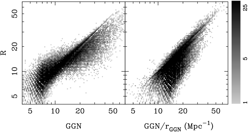
Figure 5.— Comparison between the gross galaxy number ($GGN$, left) and $GGN/r_{\rm GGN}$ (right) with cluster richness. The density of cluster sample is indicated by grey in the plot.

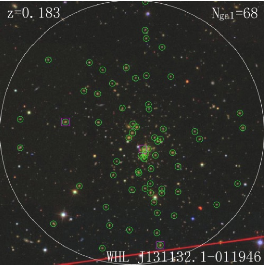
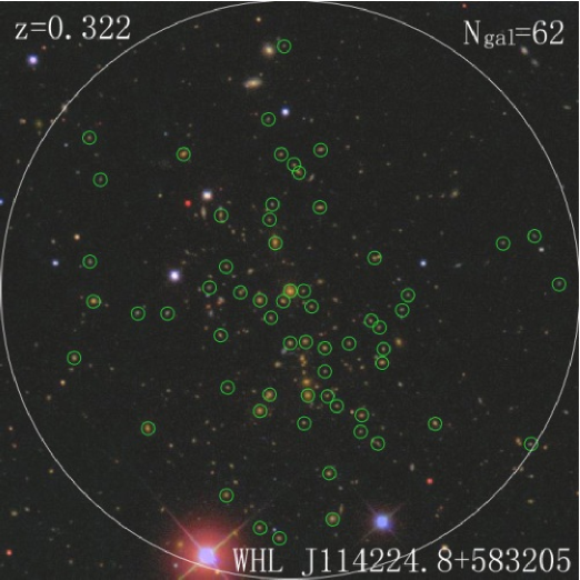
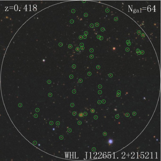
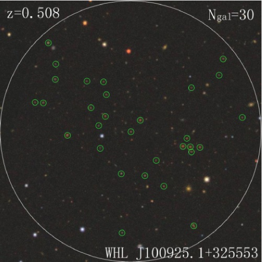
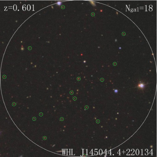
Figure 6.— Examples of detected clusters at different redshifts and their member galaxies discrimination. The big circle on the image has a radius of 1 Mpc from the cluster center. The small circles indicate member candidates discriminated by our method. The squares indicate member galaxies of $M_{r}\leq-21$ with velocities differing from that of the cluster by less than 4500 km s^-1 in the SDSS spectroscopic data. A color version of this figure is available in the online journal.

We detect a cluster if more than eight member galaxies of $M_{r}\leq-21$ are found within 0.5 Mpc from the cluster center. For clusters at very low redshifts, although most of the member galaxies of $M_{r}\leq-21$ can be included within the photometric redshift gap, their absolute magnitudes have large uncertainties when the estimated redshift slightly deviates from its true redshift. Therefore, we restrict our cluster detection with a lower redshift cutoff of $z=0.05$. The nearby clusters ($z<0.05$) have been easily detected in the spectroscopic redshift space (see, e.g., Miller et al., 2005).

To show overdensity of our clusters, we estimate the mean number counts of galaxies within the same criteria of our algorithm, and the root mean square (rms). At a given $z$, 2000 random positions (R.A., Decl.) are selected in the real background of galaxies. We count the number of galaxies ($M_{r}\leq-21$), $N(0.5)$, within a radius of 0.5 Mpc and a redshift gap between $z\pm 0.04(1+z)$, and then estimate the mean number count and the rms (see Figure 2). The mean number counts, $\langle N(0.5)\rangle$, is found to be $\sim$1.2 in the redshift range $0.1<z<0.42$, and the rms is also nearly constant, to be $\sigma_{N(0.5)}\sim 1.3$ at $0.1<z<0.42$. The number counts decrease at higher redshift ($z>0.42$) because the galaxy sample with a faint end of $r=21.5$ is incomplete for galaxies of $M_{r}\leq-21$. We define the overdensity level of a cluster to be $D=(N(0.5)-\langle N(0.5)\rangle)/\sigma_{N(0.5)}$. The minimum number is eight within 0.5 Mpc from a cluster center, and corresponds to a minimum overdensity level $D$ about 4.5, above which the false detection rate is very low in principle (see Section 3.4).

The number of member galaxy candidates ($N_{\rm gal}$ hereafter) is defined to be the number of galaxies ($M_{r}\leq-21$) within 1 Mpc (not 0.5 Mpc) from the cluster center in the redshift gap between $z\pm 0.04(1+z)$. The cluster richness, $R$, is defined by the number of real member galaxies in this region. It is estimated by $N_{\rm gal}$ but subtracting contamination from foreground and background galaxies. The contamination has to be estimated according to the local background for each cluster. First, for each cluster, we divide the area from its center to a radius of 3 Mpc into 36 annuluses, each with an equal area of 0.25$\pi$ Mpc², and then count the number of luminous ($M_{r}\leq-21$) galaxies within each annulus. Certainly, this is done within the redshift gap $z\pm 0.04(1+z)$. Secondly, we get the distribution peak at the count $n$ from the 36 number counts. The background is estimated from the average galaxy density in all annuluses with a number count less than $n+\sigma_{N(0.5)}\approx n+1$. More galaxies in an annulus are probably from real structures around the cluster, such as merging clusters, superclusters or cosmological web structures. The average contamination background within an annulus area of 0.25$\pi$ Mpc² is

$$\langle N_{\rm cb}\rangle=\Big{[}\sum_{i=1}^{36}N^{i}_{\rm ann}\theta(n+1-N^{i}_{\rm ann})\Big{]}\Big{/}N_{\rm ring}.$$ (1)

Here $\theta(x)$ is the step function, $\theta(x)=1$ for $x\geq 0$ and zero otherwise; $N^{i}_{\rm ann}$ is the number count within $i$th annulus; $N_{\rm ring}$ is the total number of annuluses with $N^{i}_{\rm ann}\leq n+1$. Then, the real number of cluster galaxies (richness, $R$) within a radius of 1 Mpc is estimated to be $R=N_{\rm gal}-4\times\langle N_{\rm cb}\rangle$.

We notice that for many clusters, the radius of 1 Mpc is not the boundary of luminous cluster galaxies. The boundary can be recognized from the number counts within the annuluses. It is defined to be the radius of the first annulus from a cluster center, from which two outer successive annuluses have $N^{i}_{\rm ann}\leq n+1$. We take it as the radius for member galaxy detection, $r_{\rm GGN}$, within which we count all luminous galaxies. After subtracting background, we obtain the gross galaxy number of a cluster, $GGN$.

From the SDSS DR6, we obtain 39,668 clusters (named after WHL and J2000 coordinates of cluster center) in the redshift range $0.05<z<0.6$. All clusters are listed in Table 1 (a full list is available in the online version). Figure 3 shows the redshift distribution of the clusters, compared with that of the SDSS maxBCG clusters. The distribution can be well fitted by the expected distribution for a complete volume-limited sample (the dashed line) with a number density of $7.8\times 10^{-6}$ Mpc^-3 at $z<0.42$. Above this redshift, it is less complete because of the flux cutoff at $r=21.5$ for the input galaxy sample.

Figure 4 shows the distributions of the number of member galaxy candidates within a radius of 1 Mpc, $N_{\rm gal}$, the cluster richness, $R$, and the gross galaxy number, $GGN$. The peaks are at $N_{\rm gal}\sim$16, $R\sim$10 and $GGN\sim 6$. Among 39,668 clusters listed in our catalog, 28,082 clusters (71%) have a richness $R\geq 10$, 4059 clusters (10%) have $R\geq 20$, and 610 clusters (1.5%) have $R\geq 30$.

Figure 5 compares $GGN$ and $GGN/r_{\rm GGN}$ with cluster richness. We find that $GGN$ is related to cluster richness but not linearly, while $GGN/r_{\rm GGN}$ is nearly linearly related to cluster richness. The scatter is larger at the lower end probably because of the quantized radius of annuluses, which is more uncertain at smaller radius. We notice that cluster–galaxy cross-correlation is described by a power law, $\xi(r)\propto r^{-\gamma}$, with the correlation index $\gamma\sim 2$ (e.g., Lilje & Efstathiou, 1988). Hence, the value of $GGN/r_{\rm GGN}$ is related to the amplitude of cluster–galaxy cross-correlation, which has been shown to be a tracer of cluster richness (Yee & López-Cruz, 1999). In the following, we use the richness $R$ to study the statistical properties of our catalog and compare them with other optical catalogs, but we will consider $GGN$ and $GGN/r_{\rm GGN}$ in the discussions of their correlations with X-ray properties (see Section 5.1).

Examples of six clusters at different redshifts and their member galaxies discrimination are shown in Figure 6. For the cluster WHL J155820.0$+$271400 (Abell 2142) at $z=0.091$, we get $N_{\rm gal}=56$ and $R=44$. Within a radius of 1 Mpc, 62 galaxies of $M_{r}\leq-21$ have velocities differing from that of the cluster by less than 4500 km s^-1 in the SDSS spectroscopic data (the velocity dispersion of a very rich cluster can be 1500 km s^-1). We discriminate 52 (84%) of them by using photometric redshifts. In addition, four galaxies with velocity difference greater than 4500 km s^-1 are selected as members. This example shows that photometric redshifts are reliable for member galaxies discrimination at $z\sim 0.1$. The richness of this cluster is 95 by the maxBCG method (defined to be the number of member galaxies brighter than 0.4$L^{\ast}$ within 1 $h^{-1}$ Mpc), and 164 by the method of Yang et al. (2007) (defined to be the number of member galaxies of $M_{r}\leq-19.5$). The second example is WHL J131132.1$-$011946 (Abell 1689) at $z=0.183$, for which we get $N_{\rm gal}=68$ and $R=62.74$. Only three member galaxies have spectroscopic redshifts in the SDSS. The richness of this cluster is 102 by the maxBCG method, but only two by the method of Yang et al. (2007). For clusters WHL J114224.8$+$583205 (Abell 1351) at $z=0.322$, WHL J122651.2$+$215211 (NSCS) at $z=0.418$ and WHL J100925.1$+$325553 at $z=0.508$, though no member galaxies have spectroscopic redshifts, most of the luminous member galaxies ($M_{r}\leq-21$) of these clusters can be well discriminated by using photometric redshifts. For cluster WHL J145044.4$+$220134 at $z=0.601$, 18 luminous red galaxies are discriminated. Some probable cluster galaxies are not selected as members because of poor estimate of photometric redshift at $z\sim 0.6$ (see Figure 1). In general, these examples show that photometric redshifts can be very efficient indicator for picking up cluster galaxies up to $z\sim 0.5$ in the SDSS, much deeper than that by spectroscopic redshifts.

3. Statistical tests for the identified Clusters

Using the SDSS spectroscopic redshifts, we estimate the uncertainty of cluster redshift, the contamination rate, and the completeness of discriminated member galaxies. We also examine the reliability of cluster richness determined by our method. Moreover, Monte Carlo simulations are performed with the real observed background of galaxies to estimate cluster detection rate and false detection rate of our algorithm.

3.1. Redshift test

We verify the accuracy of photometric redshifts of clusters in our catalog. The spectroscopic redshift of a cluster is taken to be that of its brightest cluster galaxy (BCG). From the SDSS data, we find BCGs of 13,643 clusters having spectroscopic redshifts measured. In Figure 7, we show the distribution of difference between photometric and spectroscopic redshifts, $z_{p}-z_{s}$. In each panel, we fit the distribution of $z_{p}-z_{s}$ with a Gaussian function. The systematic offset $\delta$ of the fitting is $-0.002$ or $-0.003$, and the standard deviation $\sigma$ is around 0.02.

Figure 7.— Distribution of the difference between photometric and spectroscopic redshifts in the four redshift ranges. The solid line is the best fit with a Gaussian function. The parameters, i.e., the offset $\delta$ and the standard deviation $\sigma$, of the Gaussian function are marked on the left of each panel.

3.2. Member detection and richness tests

Figure 8.— Completeness (the upper panel) and contamination rate (the lower panel) of member galaxy candidates within a radius of 1 Mpc against the number of member galaxy candidates, $N_{\rm gal}$.

Within photometric redshift gap, member galaxies can be contaminated by foreground and background galaxies and incompletely detected. Now, we use the spectroscopic redshifts of the SDSS DR6 to study the contamination due to projection effect and the completeness of member galaxies discrimination. From our sample, we obtain 1070 clusters with more than five discriminated members having spectroscopic redshifts. Totally, 10,677 galaxies with spectroscopic redshifts are discriminated as members of these clusters. The cluster redshift can be defined to be the median redshift of these member galaxies with spectroscopic redshifts for each of these clusters. We compare individual member redshifts with the estimate of the cluster redshift, and find that 2260 (21%) galaxies have velocity difference from clusters by more than 2000 km s^-1. They are probably not the member galaxies, and therefore are considered as contamination of galaxies. However. this percentage is somewhat biased by the SDSS spectroscopic selection. Since bright galaxies are preferentially targeted in the SDSS spectroscopic survey, the spectroscopically measured galaxies in the dense region are more likely member galaxies of clusters. Assuming that the effect of other selection bias, e.g., fiber collisions, is limited on measurement of galaxies, the fraction of 21% can be considered as a lower limit of contamination rate.

To estimate the completeness, we get the total member galaxies in the SDSS data. In the 1070 clusters, 8793 galaxies of $M_{r}\leq-21$ within 1 Mpc from cluster centers have velocities differing from those of clusters by less than 2000 km s^-1, of which 7882 (90%) galaxies have been found as member galaxies by our method. Figure 8 shows the contamination rate and the completeness of member galaxy candidates against the number of member galaxy candidates. The completeness of member galaxies is nearly constant for clusters with different richnesses. The contamination rate is roughly 20%, and slightly decreases with $N_{\rm gal}$.

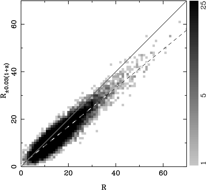
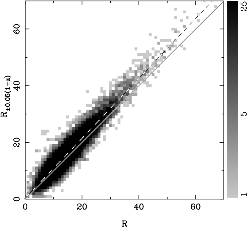
Figure 9.— Comparison between the cluster richness for the gap of $z\pm 0.04(1+z)$ and that for the gap of $z\pm 0.03(1+z)$ (the upper panel) and $z\pm 0.05(1+z)$ (the lower panel). The dashed line shows the best linear fit. The solid line is an equal line.

The contamination rate and the completeness depend on photometric redshift gap. With a larger gap, real member galaxies are selected more completely, but the member contamination becomes severer. With a smaller gap, we can discriminate less real member galaxies with a small contamination, but the sensitivity of cluster detection is lower. The gap about $z\pm 0.04(1+z)$ is a reliable compromise, within which the majority of member galaxies in a cluster can be picked out with only a small percentage of contamination galaxies included (see Figure 8). To study how the richness depends on the gap, we obtain richnesses of clusters using different photometric redshift gaps. Figure 9 compares these cluster richnesses. They are tightly correlated with relations of

$$R_{\pm 0.03(1+z)}=(0.67\pm 0.01)+(0.81\pm 0.01)\times R,$$ (2)

and

$$R_{\pm 0.05(1+z)}=(0.33\pm 0.01)+(1.06\pm 0.01)\times R.$$ (3)

Statistically, the tight correlations suggest that any richness within a gap between $z\pm 0.03(1+z)$ and $z\pm 0.05(1+z)$ can be an equivalent indicator of true richness. The richness does not change much for that with the gap of $z\pm 0.05(1+z)$, indicating that member galaxies are selected with a good completeness for the gap of $z\pm 0.04(1+z)$.

3.3. Cluster detection rate

Mock clusters are simulated with assumptions for their distributions and then added to the real data of the SDSS to test the detection rate of the mock clusters by our cluster-finding algorithm.

The luminosity function of galaxies in a cluster is taken to follow the Schechter function (Schechter, 1976)

$$\phi(M)dM\propto 10^{-0.4(M-M^{\ast})(\alpha+1)}\exp[-10^{-0.4(M-M^{\ast})}]dM.$$ (4)

We adopt the parameters as, $\alpha=-0.85\pm 0.03$, $M^{\ast}=-22.21\pm 0.05$, derived by Goto et al. (2002b) based on the SDSS CE clusters. We also assume that the galaxy number density in a mock cluster follows the Navarro-Frenk-White (NFW) profile (Navarro et al., 1997), in which the scaled radius is adopted to be 0.25 Mpc (for clusters with masses of $\sim$$10^{14}$ $M_{\odot}$; see Pointecouteau et al., 2005). The mock clusters are distributed in redshift space with a uniform comoving number density. Then, we calculate the apparent magnitudes of cluster galaxies after correcting their colors in the $r$ band with the $K$-correction curve of early-type galaxy by Fukugita et al. (1995). The photometric redshifts are assigned to the member galaxies of each cluster. We assume that the uncertainty of photometric redshift of cluster galaxies follows a Gaussian probability function with a standard deviation of $\sigma_{z}$, but varies with redshift in the form of $\sigma_{z}=\sigma_{0}(1+z)$.

Figure 10.— Detection rate of mock clusters as a function of redshift in the real background for input richness of $N_{\rm in}=8$ (the open circle), 12 (the open square), 16 (the black triangle), and 20 (the black square) assuming $\sigma_{z}=0.03(1+z)$.

We do two tests. First, we test with mock clusters for different given richness independently. Here, the input richness for a mock cluster, $N_{\rm in}$, is defined to be the numbers of luminous galaxies ($M_{r}\leq-21$) within a radius of 1 Mpc. For each richness, 2000 clusters are simulated in the redshift range $0.05<z<0.55$ via above procedures assuming $\sigma_{z}=0.03(1+z)$, and added to the real SDSS data of 500 deg². Mock clusters are put to a region where no real detected cluster exists within 3 Mpc. Our cluster finding algorithm is then performed to detect these mock clusters from the galaxy sample of $r\leq 21.5$.

A mock cluster is detected if the number of recognized member galaxies ($M_{r}\leq-21$) is above the detection threshold of eight within a radius of 0.5 Mpc and the redshift gap (see Section 2.2). Here, the recognized members can be not only the member galaxies of mock clusters, but also the contamination galaxies from the real background. We emphasize again that the input richness $N_{\rm in}$ and output richness $R$ is for a radius of 1 Mpc, but the detection threshold is designed within a radius of 0.5 Mpc. Figure 10 shows the detection rates as a function of redshift for mock clusters with different input richness. The detection rates depend on input richness, but do not vary much with redshift at $z<0.4$. The detection rates of clusters with input richness of $N_{\rm in}=8$ (the open circles) are about 10% up to $z\sim 0.4$. The detection rates increase to 35% for clusters of $N_{\rm in}=12$ (the open square), and more than 60% for clusters of $N_{\rm in}=16$ (the black triangle) and 90% for $N_{\rm in}=20$ (the black square) up to $z\sim 0.4$. The detection rates decrease at a higher redshift due to the magnitude cutoff, as mentioned in Section 2.2.

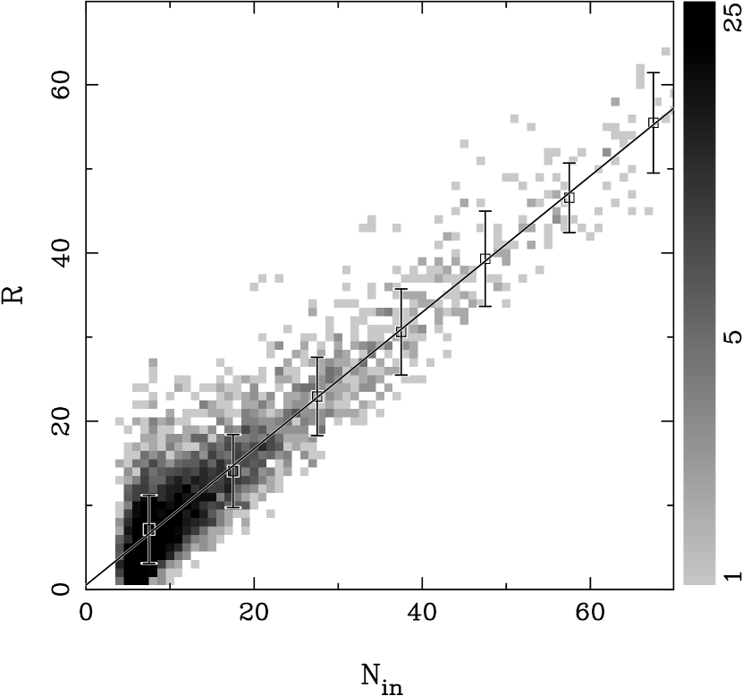
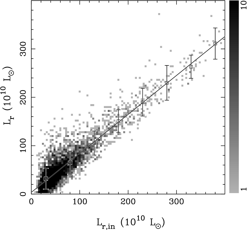
Figure 11.— Comparison between the input and output richness (the upper panel), and the input and output summed luminosity (the lower panel) for clusters of $z<0.42$.

Figure 12.— Detection rate as a function of input richness at $z<0.42$ for all detected clusters (the solid line) and more restrictively excluding those with more than half contamination (the dashed line).

Figure 13.— Upper panel: Output richness distribution of detected clusters for different input richness. Lower panel: Probability distribution of input richness for clusters that have the same output richness.

Figure 14.— Detection rate of mock clusters as a function of redshift for different output richnesses.

Secondly, we perform Monte Carlo simulation considering a population of clusters with various input richness. Using the mass function of Jenkins et al. (2001) in a cosmology with $\Omega_{m}=0.3$ and $\sigma_{8}=0.9$, we generate the halos with masses greater than $10^{14}~{}M_{\odot}$ in the redshift range $0.05<z<0.55$. According the halo occupation distribution obtained by Yang et al. (2008), we derive the number of the galaxies of ${}^{0.1}M_{r}-5\log h\leq-20$ in the halos. Here, ${}^{0.1}M_{r}$ refers to the absolute magnitude $K$-corrected and evolution corrected to $z=0.1$ in the $r$-band. The magnitudes, coordinates, redshifts and cluster input richness are simulated as described above. These mock galaxies are added to the real background, and then we detect them using our cluster-finding algorithm.

For every input cluster, we discriminate the luminous “member galaxies” ($M_{r}\leq-21$) by using photometric redshifts and obtain the output richness. We also estimate its luminosity by summing luminosities of “member galaxies” after contamination subtraction. In Figure 11, we compare the input and output richnesses and the summed luminosities for clusters of $z<0.42$. The output richness is well related to the input richness with a scatter of $\sim$5. The best fit gives

$$R=(0.52\pm 0.81)+(0.81\pm 0.01)N_{\rm in}.$$ (5)

Similar, the output summed luminosity is also well related to the input luminosity a scatter of $\sim$30$\times 10^{10}~{}L_{\odot}$. The best fit gives

$$L_{r,10}=(3.58\pm 2.39)+(0.81\pm 0.01)L_{r,\rm in,10}.$$ (6)

Here $L_{r,10}$ refers to the summed $r$-band luminosity in unit of $10^{10}~{}L_{\odot}$.

Again, a mock cluster is detected by our algorithm if more than eight luminous “member galaxies” are found within a radius of 0.5 Mpc. Figure 12 shows the detection rate as a function of input richness for clusters of $z<0.42$. The detection rate is 10% for clusters of $N_{\rm in}=8$ if all detected clusters are considered. However, if the number of member candidates of a detected cluster is more than twice of the input richness, then more than half member candidates are contamination galaxies. One can consider it as a false detection of a cluster. The detection rate becomes 6% if more restrict criterion for cluster detection is applied. The detection rate reaches 60% for clusters of $N_{\rm in}=16$, and 90% for clusters of $N_{\rm in}=20$, respectively.

In Figure 13, we show the output richness distribution of detected clusters for different input richness and the probability distribution of input richness for clusters that have the same output richness. Clusters with larger output richnesses are from larger input clusters. About 80% of detected clusters of $R=12$ are mock clusters of $N_{\rm in}\leq 16$, while about 70% detected clusters of $R=16$ are mock clusters of $N_{\rm in}\geq 16$. The detection rates by our algorithm for different output richnesses are shown in Figure 14. The detection rates are $\sim$40% for clusters of $R=12$, which increase to $\sim$60% for clusters of $R=16$ and $\sim$90% for clusters of $R=20$. As one can see from Figure 11, clusters with input richness $N_{\rm in}\leq 12$ can have output richness $R\geq 16$ due to contamination from real background. Since there are significantly more relatively poorer clusters than big ones, many clusters of $R\geq 16$ in the output catalog would be poor ones if the detection threshold (i.e., eight galaxies within a radius of 0.5 Mpc) is not used. Our algorithm preferentially detects the rich clusters as shown above, and hence reduces the contamination from the poor clusters in the output catalog. The above simulations show that the completeness of cluster detection by our method is nearly constant up to $z\sim 0.42$ using photometric redshift catalog of the SDSS. The output catalog is $\sim$60% complete for clusters with $N_{\rm in}=16$, and $\sim$90% complete for clusters with $N_{\rm in}=20$.

3.4. False detection rate

The presence of the large-scale structures makes it possible to detect false clusters because of projection effect. We also perform Monte Carlo simulation with the real SDSS data to estimate the false detection rate. Our method is similar to that of Goto et al. (2002a). First, each galaxy in the real SDSS data is forced to have a random walk in the two-dimension projected space in a random direction. The step length is a random value less than 2.5 Mpc. Second, we shuffle the photometric redshift of the galaxy sample. The procedures above are to eliminate the real clusters, but reserve the larger scale structure in two-dimension projected space. The maximum step of 2.5 Mpc is chosen so that clusters as rich as $N_{\rm gal}=100$ can be eliminated. Our method is applied to detect “clusters” from the shuffled sample of 500 deg².

Figure 15 shows the distribution of the number counts of galaxies ($M_{r}\leq-21$) within 0.5 Mpc from the centers of “cluster” candidates and the photometric redshift gap of $z\pm 0.04(1+z)$. Only 148 “clusters” are found to exceed the threshold (the dashed line), comparing to the 2380 real detected clusters in the 500 deg² region. We cross-identify the “clusters” with real clusters within a radius of 1 Mpc, and find that 41 “clusters” match the real clusters, which means that they are clusters not well shuffled to a good randomness. The rest 107 clusters are considered as false clusters. This simulation shows that our algorithm gives a false detection rate of clusters as $107/2380\simeq$5%. The rate decreases with increase in the cluster richness as shown in Figure 16. We also take the maximum step length of 4 Mpc, and the false detection rate becomes $72/2380\simeq$3%.

Figure 15.— Distribution of the number of galaxies ($M_{r}\leq-21$) within 0.5 Mpc from “cluster center” and a redshift gap between $z\pm 0.04(1+z)$ in the shuffled data. The dashed line represents the threshold to identify clusters.

Figure 16.— False detection rate as a function of cluster richness.

4. Comparison with previous optical-selected cluster catalogs

We compare our cluster catalog with previous catalogs, the Abell, the SDSS CE, and the maxBCG catalogs. The Abell catalog contains most of rich clusters at $z<0.2$ but without a quantitative measurement of completeness (Abell et al., 1989). The SDSS CE catalog contains poor clusters as well as rich ones at $z<0.44$ (Goto et al., 2002a). The SDSS maxBCG catalog has a uniform selection in the redshift range $0.1<z<0.3$ (Koester et al., 2007b).

4.1. Comparison with the Abell clusters

Figure 17.— Upper panel: Comparison between the Abell richness and the richness we determine for the matched clusters. Lower panel: Distributions of richness for the matched and not-matched clusters.

There are 1594 Abell clusters in the sky region of the SDSS DR6. Some Abell clusters have redshifts not measured previously. We take their redshifts to be the values of the BCGs from the SDSS data. The photometric redshifts are used if no spectroscopic redshifts are available. Totally, 1354 Abell clusters have redshifts $z>0.05$, of which 991 clusters are found within a projected separation of $r_{p}<1$ Mpc and redshift difference of $\Delta z<0.05$ (about 2.5 $\sigma$ of our cluster redshift accuracy) from clusters in our catalog. Another 53 Abell clusters are found within a projected separation of $1.0<r_{p}<1.5$ Mpc and redshift difference of $\Delta z<0.05$ from clusters in our catalog, which are likely to have substructures so that centers are defined at different substructures in two catalogs. In total, 1044 (77%) Abell clusters are considered to be matched with our catalog.

In Figure 17, we compare the Abell richness with the richness we determine for the matched clusters. The correlation is poor. The discrepancy may come from the uncertainties of the Abell richness. Yee & López-Cruz (1999) showed that the Abell richness for clusters of $z\geq 0.1$ is not a good indicator of their true richness, and sometimes the richness is overestimated by as much as a factor of 3. One reason is the Abell richness suffers from the projection effect. Simulation shows that cluster surveys in two dimensions are heavily contaminated by projection biases if the cluster search radius is as large as Abell radius of 1.5 $h^{-1}$ Mpc (van Haarlem et al., 1997). Another reason for the null correlation may be the uncertainty of the definition. Recall that the Abell richness is defined to be the number of galaxies within 2 mag range below the third-brightest galaxy within Abell radius after correcting background. The richnesses are calculated within various absolute magnitude range because the magnitudes of the third-brightest galaxies vary a lot. For the non-matched Abell clusters, we also determine their richnesses by our method. The matched Abell clusters have a high richness, while the not-matched clusters are relatively poor with richness around eight, few larger than 20 (see the lower panel of Figure 17).

4.2. Comparison with the SDSS CE clusters

Figure 18.— Fraction of the CE clusters we detected as a function of redshift.

Figure 19.— Same as Figure 17 but for the CE clusters.

The SDSS CE clusters were identified by using 34 color cuts. The redshifts of clusters were estimated with the uncertainties of $\sigma=0.0147$ at $z<0.3$ and $\sigma=0.0209$ at $z>0.3$. The CE richness is defined to be the number of galaxies within 2 mag range below the third-brightest galaxy and within the detection radius after correcting background (Goto et al., 2002a).

Among 4638 CE clusters, 1160 clusters are found within a projected separation of $r_{p}<1.5$ Mpc and redshift difference of $\Delta z<0.05$ from clusters in our catalog. Figure 18 shows the detection rates of the CE clusters by our method as function of redshift. The rates are about 20%–30% for the whole sample, and increase to 40%–50% for clusters with the CE richness $\geq 20$. The correlation between our richness and the CE richness is also poor (see Figure 19), suggesting that the CE richness has a large uncertainty. For the not-matched CE clusters, we determine their richness by our method and find that most of the not-matched clusters are relatively poor with mean richness $\sim$3 (see the lower panel of Figure 19). Obviously, the CE clusters we detected are much richer than the not-matched clusters.

4.3. Comparison with the SDSS maxBCG clusters

Figure 20.— Same as Figure 18 but for the maxBCG clusters.

Figure 21.— Same as Figure 17 but for the maxBCG clusters. $R^{\prime}$ refers to cluster richness by our method using the same radius and magnitude range with the maxBCG clusters. The solid line is an equal line.

The SDSS maxBCG is approximately 85% complete in the redshift range $0.1<z<0.3$ with masses $M>1\times 10^{14}~{}M_{\odot}$ (Koester et al., 2007b). The redshifts of clusters were estimated with the uncertainties of $\sigma=0.01$. The cluster richness, $N_{\rm gal}^{\rm max}$, is defined to be the number of galaxies within a radius of 1 $h^{-1}$ Mpc and $2\,\sigma_{c}$ of the ridgeline colors, brighter than $0.4L^{\ast}$. A scaled richness, $N_{200}$, is measured to be the number of galaxies within $r_{200}$ and the color cuts. Here, $r_{200}$ is the radius within which the mean mass density is 200 times that of the critical cosmic mass density. Among 13,823 maxBCG clusters, 6424 clusters are found within a projected separation of $r_{p}<1.5$ Mpc and redshift difference $\Delta z<0.05$ from the clusters in our catalog. As shown in Figure 20, the detection rates of the maxBCG clusters by our method are 40%–50% for the whole sample, and increase 70%–80% for clusters with the maxBCG richness $\geq 20$.

The luminosity cutoff, $0.4L^{\ast}$, of the maxBCG method corresponds to absolute magnitude of $M_{r}\simeq-20.6$ (Koester et al., 2007b), which is about 0.4 magnitude fainter than that of our work. To make a comparison, we calculate the richness, $R^{\prime}$, for the matched clusters within the same radius and magnitude range with the maxBCG clusters, i.e., 1 $h^{-1}$ Mpc and $M_{r}\leq-20.6$. In Figure 21, we compare the maxBCG richness, $N_{\rm gal}^{\rm max}$, with the richnesses, $R$ and $R^{\prime}$. Both correlations are tighter than those with the Abell and CE clusters, though large scatters exist. With the same selection criteria, we find that the maxBCG richness is systematically smaller than the richness by our method. The discrepancy may come from some systematic bias in maxBCG method. Recall that the maxBCG method only selects ridgeline member galaxies without contamination subtraction. The color–magnitude diagrams (e.g., Miller et al., 2005) show that many member galaxies fall outside of the ridgeline of red galaxies, and hence they are likely missed by the maxBCG method. Rozo et al. (2008) also pointed out the systematic bias for the maxBCG richness due to color off-sets. The ridgeline galaxies fall outside the color cuts because of the increasing photometric errors with redshift. In addition, the ridgeline of red galaxies is not as flat as assumed and even evolves with redshift, so that the color cuts based on the BCGs colors will lose some of the less luminous cluster member galaxies. Furthermore, the study by Donahue et al. (2002) shows that some massive clusters do not have a prominent red sequence, which could induce bias in cluster detection and richness measurement.

We show that our method tends to detect the rich maxBCG clusters and that the not-matched maxBCG clusters are relatively poor with mean richness $\sim$6 (see the lower panel of Figure 21).

5. Correlations of our clusters with X-ray Measurements

The measurements in X-rays provide the properties of clusters from hot intracluster gas. The imaging observations can give the X-ray luminosity, and spectroscopic observations can provide the temperature of hot gas. Using the measurements in X-rays, the gravitational cluster mass can be derived (Wu, 1994; Reiprich & Böhringer, 2002). With luminous member galaxies well discriminated, the correlations between these X-ray measurements and the cluster richness or the summed optical luminosities are expected.

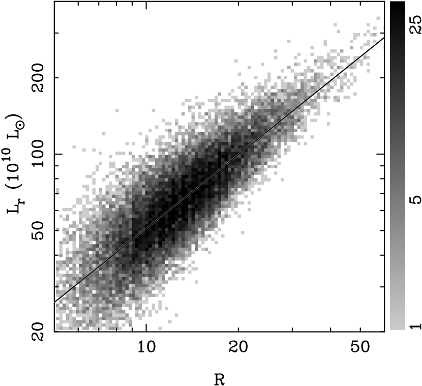
Figure 22.— Correlation between the richness and the summed luminosity for clusters of $z\leq 0.42$. The solid line is the best power-law fit given in Equation (7).

As mentioned above, the faint end of member galaxies is $M_{r}=-21$ in our sample at $z\leq 0.42$. At higher redshifts, the faint end moves to a brighter magnitude depending on redshift, so that the estimated summed luminosities for clusters of $z>0.42$ are biased. Therefore, we only consider clusters of $z\leq 0.42$ in the following statistics.

Figure 22 shows the correlation between the richness and the summed luminosities for clusters of $z\leq 0.42$. We find that the summed luminosity of a cluster is linearly related to the cluster richness by

$$L_{r,10}=(5.47\pm 0.06)R^{0.97\pm 0.01}.$$ (7)

This is consistent with the relation found by Popesso et al. (2007).

Figure 23.— Distribution of projected separations between X-ray peaks of clusters and the optical BCGs.

Figure 24.— Correlations between the cluster richness ($R$, the left panels) and summed $r$-band luminosity ($L_{r}$, the right panels) with the X-ray luminosity (the upper panels) of 146 clusters from Böhringer et al. (2000, 2004), and temperature (the bottom panels) of 67 clusters from Fukazawa et al. (2004). The lines are the best fit given in Equations (8)–(11).

5.1. Correlations between the richness and optical luminosity with the X-ray luminosity and temperature

There are 239 (203 NORAS and 36 REFLEX) X-ray clusters from Böhringer et al. (2000, 2004) in the sky region of the SDSS DR6, of which 190 clusters have redshifts $z>0.05$. We find 146 ROSAT X-ray clusters within a projected separation of $r_{p}<1.5$ Mpc and the redshift difference of $\Delta z<0.05$ from clusters in our sample. The X-ray emission of clusters usually traces the centers of matter distributions. They are likely coincident with the BCGs probably located near the centers of clusters. Figure 23 shows the distribution of the projected separation between X-ray peaks of clusters and the optical BCGs. Most (132/146) of the clusters have a separation of $r_{p}\leq 0.3$ Mpc. The small offsets are probably due to the movement of BCGs with respect to the cluster potential (Oegerle & Hill, 2001). Five merging clusters have projected separations of $r_{p}\geq 0.5$ Mpc because the BCGs and X-ray peak are located at different subclusters.

We find that the richness and summed $r$-band luminosities of 146 X-ray clusters are well correlated with the X-ray luminosity (Böhringer et al., 2000, 2004) derived from the ROSAT observations (see Figure 24). The best fit to the data gives

$$\log L_{X,44}=(-3.50\pm 0.17)+(2.79\pm 0.13)\log R,$$ (8)

and

$$\log L_{X,44}=(-5.19\pm 0.25)+(2.67\pm 0.12)\log L_{r,10}.$$ (9)

where $L_{X,44}$ refers to X-ray luminosity in the 0.1–2.4 keV band in unit of $10^{44}~{}{\rm erg~{}s^{-1}}$. The tight correlations suggest that the member galaxies are well discriminated by our method, as shown in Section 3.2. Popesso et al. (2005) studied the correlations between the optical and X-ray measurements using the RASS–SDSS clusters. They obtained the slope of the $L_{X,44}$–$L_{r,10}$ relation to be $1.72\pm 0.09$, much smaller than our result. Using maxBCG clusters, Rykoff et al. (2008) studied the mean and scatter of the $L_{X,44}$–$N_{200}$ relation, and obtained the slope of $1.82\pm 0.05$, where $N_{200}$ are determined within different radius, $r_{200}$, for different clusters. To make a comparison, we scale the slope of their relation to that of $L_{X,44}$–$N_{\rm gal}^{\rm max}$, where $N_{\rm gal}^{\rm max}$ is also defined within a fixed radius. The scaling relation between $N_{200}$ and $N_{\rm gal}^{\rm max}$ is $N_{200}\propto(N_{\rm gal}^{\rm max})^{1.41\pm 0.01}$ (Koester et al., 2007a). Therefore, the $L_{X,44}$–$N_{\rm gal}^{\rm max}$ relation has a slope of 2.57$\pm$0.09, in agreement with our result. However, the correlations of the $L_{X,44}$–$R$ relation are much tighter than that shown using the maxBCG clusters (see Figure 7 of Rykoff et al., 2008).

Fukazawa et al. (2004) compiled the temperatures of $\sim$300 X-ray clusters, of which 67 clusters are found in our catalog. We plot the richness and the summed $r$-band luminosity against the X-ray temperature for 67 clusters in Figure 24 and find the best fit as

$$\log T_{X}=(-0.40\pm 0.12)+(0.75\pm 0.08)\log R,$$ (10)

and

$$\log T_{X}=(-1.09\pm 0.18)+(0.83\pm 0.08)\log L_{r,10},$$ (11)

where $T_{X}$ refers to X-ray temperature in unit of keV. The slope of the $T_{X}$–$L_{r}$ relation is slightly higher than $0.61\pm 0.03$ found by Popesso et al. (2005).

Figure 25.— Correlations between the cluster $GGN$ (the left panels) and $GGN/r_{\rm GGN}$ (the right panels) with the X-ray luminosity (the upper panels) and temperature (the bottom panels). The lines are the best fit.

We also find the correlations between the $GGN$ and $GGN/r_{\rm GGN}$ of clusters with the X-ray luminosity and temperature. Figure 25 shows the correlations. $GGN/r_{\rm GGN}$ is more tightly correlated with $L_{X,44}$ and $T_{X}$ than $GGN$. The $L_{X,44}$–$GGN/r_{\rm GGN}$ relation and the $T_{X}$–$GGN/r_{\rm GGN}$ relation are:

$$\log L_{X,44}=(-3.92\pm 0.23)+(3.0\pm 0.17)\log(GGN/r_{\rm GGN}),$$ (12)

and

$$\log T_{X}=(-0.97\pm 0.15)+(1.13\pm 0.10)\log(GGN/r_{\rm GGN}),$$ (13)

where $GGN/r_{\rm GGN}$ is in unit of Mpc^-1.

Most of the cluster richnesses are determined based on the galaxy count (e.g., Abell et al., 1989). Other efforts were made to measure the richness of cluster by various methods, e.g., correlation function amplitude of the galaxies and the matched filter richness (Yee & López-Cruz, 1999; Rozo et al., 2008). However, few measured richnesses tightly correlate with measurements in X-rays due to the lack of accurate membership discrimination. With membership discrimination using photometric redshift, we show tighter correlations between the measurements of clusters in optical and X-ray bands. Obviously, the accuracy membership discrimination is crucial for finding the scaling relation of clusters.

5.2. Correlations of the richness and optical luminosity with the cluster mass

Figure 26.— Correlations between the cluster richness (the left panel) and summed $r$-band luminosity (the right panel) with cluster mass from Reiprich & Böhringer (2002) for 24 clusters. The lines are the best fit given in Equations (14)–(15)

The X-ray luminosity and temperature have been found to be tightly correlated with cluster mass (Finoguenov et al., 2001; Allen et al., 2001; Xu et al., 2001; Reiprich & Böhringer, 2002; Shimizu et al., 2003). As shown, the cluster richness and summed luminosity are well correlated with X-ray luminosity and temperature, hence can also trace cluster mass.

We obtain cluster masses, $M_{200}$, determined from X-ray measurements by Reiprich & Böhringer (2002). Here, $M_{200}$ is the total mass within the radius $r_{200}$. Among the sample of Reiprich & Böhringer (2002), there are 28 clusters/groups in the sky region of SDSS DR6. We exclude four nearby groups ($z\leq 0.006$), which contain only one luminous elliptical galaxies. Therefore, we have masses of 24 clusters in the redshift range $0.02<z<0.2$, of which 12 clusters are found in our catalog. To determine the $M_{200}$–$L_{r}$ and $M_{200}$–$R$ relations precisely, we also calculate the richness and summed $r$-band luminosities for the rest 12 clusters by our method. We plot the richness and the summed luminosity against the cluster masses for 24 clusters in Figure 26 and find the best fit as

$$\log\Big{(}\frac{M_{200}}{10^{14}~{}M_{\odot}}\Big{)}=(-2.08\pm 0.06)+(1.90\pm 0.04)\log R,$$ (14)

and

$$\log\Big{(}\frac{M_{200}}{10^{14}~{}M_{\odot}}\Big{)}=(-2.67\pm 0.07)+(1.64\pm 0.03)\log L_{r,10}.$$ (15)

In the previous studies, the mass–richness relation (the so called halo occupation distribution in some literature) is described in a power law, $R\propto M^{\beta}$, and the factor $\beta$ is expected less than 1 from the simulations (e.g., White et al., 2001). Our result, $1/\beta=1.90\pm 0.04$, i.e., $\beta=0.53\pm 0.01$, is in agreement with $\beta=0.55\pm 0.04$ found by Marinoni & Hudson (2002), but significantly smaller than $\beta=0.70\pm 0.04$ found by Pisani et al. (2003) and $\beta=0.92\pm 0.03$ found by Popesso et al. (2007).

The correlation of cluster mass with the optical luminosity, i.e., mass-to-light ratio $M/L$, is also very interesting. Adami et al. (1998) investigated a fundamental plane in nearby rich Abell clusters and suggested that the $M/L$ is not constant. In general, the $M/L$ is also described by a power law, $M/L\propto L^{\tau}$, with $\tau$ in the range 0.2–0.4 (Bahcall & Comerford, 2002; Girardi et al., 2002; Lin et al., 2003; Rines et al., 2004; Popesso et al., 2005). Our result, $\tau+1=1.64\pm 0.03$, i.e., $\tau=0.64\pm 0.03$, is larger than the normal $\tau$ range, but smaller than $\tau=0.8$ found by Bardeau et al. (2007).

Recall that our cluster finding algorithm can detect 60% clusters of $N_{\rm in}=16$, which corresponds to a mean output richness $R=13.5$ according to Equation (5). The rate increases to 90% for clusters of $N_{\rm in}=20$ with a mean $R=16.7$. Using Equation (14), the output catalog is therefore 60% complete for clusters with a mass $M_{200}\sim 1.2\times 10^{14}~{}M_{\odot}$, and 90% complete for clusters with a mass $M_{200}\sim 2\times 10^{14}~{}M_{\odot}$.

5.3. Candidates for New X-ray clusters

The ROSAT All Sky Survey detects 18,806 bright sources (Voges et al., 1999) and 105,924 faint sources (Voges et al., 2000) in the 0.1–2.4 keV band, of which 495 extended sources in the northern hemisphere and 447 extended sources in the southern hemisphere have been identified as clusters and AGNs or stars (Böhringer et al., 2000, 2004).

We cross-identify the ROSAT X-ray bright and faint sources with clusters in our catalog to find new candidates for X-ray clusters. Only those X-ray sources with a projected separation of $r_{p}<0.3$ Mpc from the BCGs are probably associated with clusters (see Figure 23). The hardness ratios are expected in the range 0–1 for clusters (Böhringer et al., 2000), which can help to distinguish the cluster X-ray sources. The X-ray sources with hardness ratios out of 0–1 can be excluded to be associated with clusters. Figure 27 shows the distribution of a projected separation between the X-ray sources and the BCGs of clusters in our catalog. If the X-ray sources are uncorrelated with the clusters, the number of pairs in each $r_{p}$ bin is proportional to $r_{p}^{2}$. The number excess at low $r_{p}$ suggests that many of the X-ray sources are clusters.

912 clusters in our catalog have a ROSAT X-ray source within $r_{p}<0.3$ Mpc, and 227 of them are known X-ray clusters according to NASA/IPAC Extragalactic Database. The rest 685 clusters are new candidates for X-ray clusters. We notice that the candidate distribution becomes constant within $0.5<r_{p}<1$ Mpc (see Figure 27). The real number of X-ray clusters should be the excess over the constant level, them about 60% of new candidates are expected to be real X-ray clusters. We also show the redshift distribution of the new candidates for X-ray cluster together with that of known ROSAT X-ray clusters from Böhringer et al. (2000, 2004) in the lower panel of Figure 27. Hundreds of candidates have redshifts $z>0.3$. We list both 685 new candidates and 227 known X-ray clusters in Table 2 (a full list is available in the online version).

Figure 27.— Upper panel: Distribution of projected separations between ROSAT X-ray sources and the BCGs of clusters in our catalog. Lower panel: Redshift distribution of the candidates for X-ray clusters ($r_{p}<0.3$ Mpc, solid histogram). The dotted histogram is for the known ROSAT X-ray clusters .

6. Summary

We identify 39,668 clusters of galaxies in the redshift range $0.05<z<0.6$ using photometric redshifts of galaxies from the SDSS DR6. A cluster is recognized if more than eight member galaxies of $M_{r}\leq-21$ are found within a radius of 0.5 Mpc and a photometric redshift gap between $z\pm 0.04(1+z)$. This is the largest cluster catalog to date. Our sample is much deeper in redshift than the previous cluster catalogs from the SDSS. Cluster redshifts are estimated with an uncertainty less than 0.022. Using the SDSS spectroscopic data, we also estimate the contamination rate and completeness of member galaxy candidates to be about 20% and 90%, respectively. Monte Carlo simulations show that the cluster detection rate depends on richness, but is approximately constant to redshift $z=0.42$. The detection rate is $\sim$60% for clusters with a mass $M_{200}\sim 1.2\times 10^{14}~{}M_{\odot}$, which corresponds to a mean output richness $R\sim 13.5$. The detection rate increases to be 90% for clusters with a mass $M_{200}>2\times 10^{14}~{}M_{\odot}$, which corresponds to a mean $R\sim 16.7$. The false detection rate of clusters is $\sim$5% for our algorithm.

We compare our catalog with the published Abell, CE, maxBCG, and ROSAT X-ray cluster catalogs. We find that our catalog includes 77% Abell clusters and 77% ROSAT X-ray selected clusters at $z>0.05$. Rich clusters are more likely detected by our method.

With luminous member galaxies discriminated, we get the richness, $R$, the summed luminosity, $L_{r}$, and the gross galaxy number $GGN$ within a cluster radius ($r_{\rm GGN}$) for clusters in our catalog up to $z\sim 0.42$. We find that they are tightly related to the X-ray luminosity and temperature, and can trace the cluster mass with the relations, $M_{200}\propto R^{1.90\pm 0.04}$ and $M_{200}\propto L_{r}^{1.64\pm 0.03}$. By cross-identification with the ROSAT X-ray source list, we obtain 685 new candidates of X-ray clusters, of which 60% are likely true.

Table 139668 Clusters identified from the SDSS DR6

Name	R.A.BCG	Decl.BCG	$z_{p}$	$z_{s,\rm BCG}$	$r_{\rm BCG}$	Ngal	R	$GGN$	$r_{\rm GGN}$	$L_{r}$	$D$	Other catalogs
	(deg)	(deg)							(Mpc)	($10^{10}L_{\odot}$)
(1)	(2)	(3)	(4)	(5)	(6)	(7)	(8)	(9)	(10)	(11)	(12)	(13)
WHL J000006.0$+$152547	0.02482	15.42990	0.1735	$-1.0000$	16.58	15	11.30	9.07	0.50	62.69	6.97	maxBCG
WHL J000007.1$-$092909	0.02957	$-9.48607$	0.3963	$-1.0000$	19.11	19	15.88	14.44	0.71	81.33	8.56
WHL J000007.6$+$155003	0.03177	15.83423	0.1489	0.1528	16.00	17	13.40	13.20	0.71	54.61	6.55	Abell,maxBCG
WHL J000020.1$+$160859	0.08358	16.14976	0.4591	$-1.0000$	19.88	20	18.56	29.40	1.58	107.01	6.02
WHL J000021.7$+$150611	0.09053	15.10328	0.2883	$-1.0000$	17.67	20	18.17	22.88	1.50	94.66	9.43	maxBCG
WHL J000025.1$-$093452	0.10453	$-9.58125$	0.3648	$-1.0000$	18.44	16	9.29	9.65	0.71	74.32	4.90
WHL J000027.6$-$010140	0.11617	$-1.04317$	0.4491	0.4387	18.62	25	20.07	20.07	1.00	124.10	8.81
WHL J000048.3$-$011204	0.18509	$-1.20016$	0.4373	0.4392	18.76	18	14.44	13.33	0.87	82.12	5.01
WHL J000050.5$+$004705	0.21051	0.78477	0.2458	$-1.0000$	17.64	22	20.10	26.16	1.22	105.53	5.94	NSCS,CE,maxBCG
WHL J000050.7$+$004704	0.21134	0.78470	0.4889	$-1.0000$	19.73	10	6.40	7.10	0.50	51.92	5.69
WHL J000052.9$+$160520	0.22045	16.08902	0.1986	$-1.0000$	16.88	12	10.22	11.33	1.22	46.42	5.44
WHL J000059.1$+$004841	0.24642	0.81162	0.3551	$-1.0000$	19.18	18	14.80	13.60	0.87	70.64	4.93	NSCS
WHL J000111.3$+$151839	0.29608	15.30418	0.4053	$-1.0000$	19.10	21	19.10	30.26	1.58	125.22	6.50
WHL J000116.2$-$093137	0.31767	$-9.52720$	0.3383	0.3693	18.29	24	19.83	31.65	1.41	112.56	7.03
WHL J000117.5$+$142848	0.32297	14.48012	0.3815	$-1.0000$	19.68	17	12.84	11.92	0.71	45.04	4.93

Note. — Column (1): Cluster name with J2000 coordinates of cluster center; Column (2): R.A. (J2000) of cluster BCG; Column (3): Decl. (J2000) of cluster BCG; Column (4): photometric redshift of cluster; Column (5): spectroscopic redshift of cluster BCG, $-1.0000$ means not available; Column (6): $r$-band magnitude of cluster BCG; Column (7): number of member galaxy candidates within 1 Mpc; Column (8): cluster richness; Column (9): gross galaxy number; Column (10): radius of member galaxy detection (Mpc); Column (11): summed $r$-band luminosity of cluster; Column (12): overdensity level of cluster; Column (13): Other catalogs containing the cluster: Abell (Abell, 1958; Abell et al., 1989); Zwcl (Zwicky et al., 1968); CE (Goto et al., 2002a); NSC (Gal et al., 2003); NSCS (Lopes et al., 2004); maxBCG (Koester et al., 2007b); RXC (Böhringer et al., 2000, 2004).

This table is available in its entirety in a machine-readable form in the online journal. A portion is shown here for guidance regarding the form and content.

The original catalog published in ApJS contains 39,716 clusters. Thanks Dr. Heinz Andernach for pointing out repeated entries (caused by a found bug in very early version of a code). We hence revised this table, and removed 48 entries and corrected BCG positions of 296 clusters.

Table 2912 clusters with ROAST X-ray sources including 685 candidates and 227 known X-ray clusters.

Name of X-ray source	Cluster Name	R.A.BCG	Decl.BCG	$z_{p}$	$r_{p}$	Count rate	Known X-ray clusters
		(deg)	(deg)		(Mpc)	(count s-1)
(1)	(2)	(3)	(4)	(5)	(6)	(7)	(8)
RXS J000522.7$+$161306	WHL J000524.0$+$161309	1.34987	16.21922	0.1115	0.04	0.076	RXC
RXS J001739.4$-$005150	WHL J001740.0$-$005314	4.40670	$-0.87835$	0.2340	0.21	0.037
RXS J002302.3$+$144645	WHL J002300.7$+$144656	5.75279	14.78240	0.3826	0.13	0.033
RXS J002815.2$+$135601	WHL J002819.8$+$135459	7.08254	13.91657	0.1516	0.23	0.026
RXS J003209.2$-$003932	WHL J003212.1$-$003950	8.04672	$-0.66670$	0.2175	0.14	0.013
RXS J003417.8$+$005145	WHL J003419.1$+$004948	8.59684	0.85723	0.2035	0.27	0.024
RXS J004149.7$-$091817	WHL J004148.2$-$091703	10.46029	$-9.30313$	0.0560	0.01	4.079	RXC
RXS J010101.1$-$095726	WHL J010101.5$-$095717	15.25645	$-9.95473$	0.1457	0.03	0.035
RXS J010243.0$+$010805	WHL J010243.1$+$010810	15.67950	1.13633	0.1345	0.01	0.052	RX
RXS J010649.5$+$010317	WHL J010650.5$+$010410	16.71051	1.06970	0.2527	0.21	0.187	RXC
RXS J010717.9$+$141635	WHL J010721.9$+$141623	16.84109	14.27322	0.0963	0.10	0.020
RXS J010921.7$+$005457	WHL J010923.1$+$005429	17.34616	0.90818	0.2723	0.14	0.029
RXS J011006.0$+$135849	WHL J011001.3$+$135555	17.51321	13.97815	0.0712	0.06	0.061	RXC
RXS J011202.7$-$004355	WHL J011204.1$-$004351	18.01689	$-0.73108$	0.2119	0.07	0.053
RXS J011940.0$+$145303	WHL J011938.3$+$145352	19.90952	14.89799	0.1289	0.12	0.096	RXC

Note. — Column (1): Name of ROSAT X-ray source with J2000 coordinates; Column (2): Cluster name in Table 1; Column (3): R.A. (J2000) of cluster BCG; Column (4): Decl. (J2000) of cluster BCG; Column (5): photometric redshift of cluster; Column (6): projected separation between X-ray source and cluster BCG in Mpc; Column (7): Count rate of X-ray cluster in 0.1–2.4 keV band; Column (8): Known X-ray clusters in the NASA/IPAC Extragalactic Database (NED).

This table is available in its entirety in a machine-readable form in the online journal. A portion is shown here for guidance regarding the form and content.

The original catalog published in ApJS contains 790 candidates of X-ray clusters, of which many known X-ray clusters in the NED were mixed in. Thanks Dr. Heinz Andernach for pointing out this problem after publication.

References

- Abell (1958) Abell, G. O. 1958, ApJS, 3, 211
- Abell et al. (1989) Abell, G. O., Corwin, Jr., H. G., & Olowin, R. P. 1989, ApJS, 70, 1
- Adami et al. (1998) Adami, C., Mazure, A., Biviano, A., Katgert, P., & Rhee, G. 1998, A&A, 331, 493
- Allen et al. (2001) Allen, S. W., Schmidt, R. W., & Fabian, A. C. 2001, MNRAS, 328, L37
- Bahcall (1988) Bahcall, N. A. 1988, ARA&A, 26, 631
- Bahcall & Comerford (2002) Bahcall, N. A. & Comerford, J. M. 2002, ApJ, 565, L5
- Bahcall et al. (1997) Bahcall, N. A., Fan, X., & Cen, R. 1997, ApJ, 485, L53
- Bahcall et al. (2003) Bahcall, N. A., McKay, T. A., Annis, J., et al. 2003, ApJS, 148, 243
- Bardeau et al. (2007) Bardeau, S., Soucail, G., Kneib, J.-P., et al. 2007, A&A, 470, 449
- Berlind et al. (2006) Berlind, A. A., Frieman, J., Weinberg, D. H., et al. 2006, ApJS, 167, 1
- Blain et al. (1999) Blain, A. W., Kneib, J.-P., Ivison, R. J., & Smail, I. 1999, ApJ, 512, L87
- Böhringer et al. (2000) Böhringer, H., Voges, W., Huchra, J. P., et al. 2000, ApJS, 129, 435
- Böhringer et al. (2004) Böhringer, H., Schuecker, P., Guzzo, L., et al. 2004, A&A, 425, 367
- Bradač et al. (2008) Bradač, M., Schrabback, T., Erben, T., et al. 2008, ApJ, 681, 187
- Bramel et al. (2000) Bramel, D. A., Nichol, R. C., & Pope, A. C. 2000, ApJ, 533, 601
- Brunner & Lubin (2000) Brunner, R. J. & Lubin, L. M. 2000, AJ, 120, 2851
- Burenin et al. (2007) Burenin, R. A., Vikhlinin, A., Hornstrup, A., Ebeling, H., Quintana, H., & Mescheryakov, A. 2007, ApJS, 172, 561
- Butcher & Oemler (1978) Butcher, H. & Oemler, Jr., A. 1978, ApJ, 219, 18
- Butcher & Oemler (1984) —. 1984, ApJ, 285, 426
- Cannon et al. (2006) Cannon, R., Drinkwater, M., Edge, A., et al. 2006, MNRAS, 372, 425
- Carlberg et al. (1996) Carlberg, R. G., Yee, H. K. C., Ellingson, E., Abraham, R., Gravel, P., Morris, S., & Pritchet, C. J. 1996, ApJ, 462, 32
- Carlstrom et al. (2000) Carlstrom, J. E., Joy, M. K., Grego, L., et al. 2000, Physica Scripta Volume T, 85, 148
- Castillo-Morales & Schindler (2003) Castillo-Morales, A. & Schindler, S. 2003, A&A, 403, 433
- Csabai et al. (2003) Csabai, I., Budavári, T., Connolly, A. J., et al. 2003, AJ, 125, 580
- Dahle (2006) Dahle, H. 2006, ApJ, 653, 954
- Dalton et al. (1997) Dalton, G. B., Maddox, S. J., Sutherland, W. J., & Efstathiou, G. 1997, MNRAS, 289, 263
- Deng et al. (2007) Deng, X.-F., He, J.-Z., Jiang, P., Luo, C.-H., & Wu, P. 2007, A&A, 474, 783
- Donahue et al. (2002) Donahue, M., Scharf, C. A., Mack, J., et al. 2002, ApJ, 569, 689
- Dong et al. (2008) Dong, F., Pierpaoli, E., Gunn, J. E., & Wechsler, R. H. 2008, ApJ, 676, 868
- Dressler (1980) Dressler, A. 1980, ApJ, 236, 351
- Ebeling et al. (1998) Ebeling, H., Edge, A. C., Bohringer, H., et al. 1998, MNRAS, 301, 881
- Eisenstein et al. (2001) Eisenstein, D. J., Annis, J., Gunn, J. E., et al. 2001, AJ, 122, 2267
- Eke et al. (2004) Eke, V. R., Baugh, C. M., Cole, S., et al. 2004, MNRAS, 348, 866
- Finoguenov et al. (2001) Finoguenov, A., Reiprich, T. H., & Böhringer, H. 2001, A&A, 368, 749
- Fukazawa et al. (2004) Fukazawa, Y., Makishima, K., & Ohashi, T. 2004, PASJ, 56, 965
- Fukugita et al. (1995) Fukugita, M., Shimasaku, K., & Ichikawa, T. 1995, PASP, 107, 945
- Gal et al. (2003) Gal, R. R., de Carvalho, R. R., Lopes, P. A. A., et al. 2003, AJ, 125, 2064
- Garilli et al. (1999) Garilli, B., Maccagni, D., & Andreon, S. 1999, A&A, 342, 408
- Geller & Huchra (1983) Geller, M. J. & Huchra, J. P. 1983, ApJS, 52, 61
- Gerke et al. (2005) Gerke, B. F., Newman, J. A., Davis, M., et al. 2005, ApJ, 625, 6
- Gioia et al. (1990) Gioia, I. M., Henry, J. P., Maccacaro, T., Morris, S. L., Stocke, J. T., & Wolter, A. 1990, ApJ, 356, L35
- Girardi et al. (2002) Girardi, M., Manzato, P., Mezzetti, M., Giuricin, G., & Limboz, F. 2002, ApJ, 569, 720
- Giuricin et al. (2000) Giuricin, G., Marinoni, C., Ceriani, L., & Pisani, A. 2000, ApJ, 543, 178
- Gladders & Yee (2000) Gladders, M. D. & Yee, H. K. C. 2000, AJ, 120, 2148
- Gladders & Yee (2005) —. 2005, ApJS, 157, 1
- Goto et al. (2002a) Goto, T., Sekiguchi, M., Nichol, R. C., et al., 2002a, AJ, 123, 1807
- Goto et al. (2003a) Goto, T., Okamura, S., Yagi, M., et al. 2003a, PASJ, 55, 739
- Goto et al. (2002b) Goto, T., Okamura, S., McKay, T. A., et al. 2002b, PASJ, 54, 515
- Goto et al. (2003b) Goto, T., Yamauchi, C., Fujita, Y., et al. 2003b, MNRAS, 346, 601
- Gunn et al. (1986) Gunn, J. E., Hoessel, J. G., & Oke, J. B. 1986, ApJ, 306, 30
- Huchra & Geller (1982) Huchra, J. P. & Geller, M. J. 1982, ApJ, 257, 423
- Ikebe et al. (1996) Ikebe, Y., Ezawa, H., Fukazawa, Y., et al. 1996, Nature, 379, 427
- Jee et al. (2007) Jee, M. J., Ford, H. C., Illingworth, G. D., et al. 2007, ApJ, 661, 728
- Kim et al. (2002) Kim, R. S. J., Kepner, J. V., Postman, M., et al. 2002, AJ, 123, 20
- Kochanek et al. (2003) Kochanek, C. S., White, M., Huchra, J., et al. 2003, ApJ, 585, 161
- Koester et al. (2007a) Koester, B. P., McKay, T. A., Annis, J., et al. 2007a, ApJ, 660, 221
- Koester et al. (2007b) Koester, B. P., McKay, T. A., Annis, J., et al. 2007b, ApJ, 660, 239
- Jenkins et al. (2001) Jenkins, A., Frenk, C. S., White, S. D. M., Colberg, J. M., Cole, S., Evrard, A. E., Couchman, H. M. P., & Yoshida, N. 2001, MNRAS, 321, 372
- Lee et al. (2004) Lee, B. C., Allam, S. S., Tucker, D. L., et al. 2004, AJ, 127, 1811
- Lilje & Efstathiou (1988) Lilje, P. B., & Efstathiou, G. 1988, MNRAS, 231, 635
- Lin et al. (2003) Lin, Y.-T., Mohr, J. J., & Stanford, S. A. 2003, ApJ, 591, 749
- Lopes et al. (2004) Lopes, P. A. A., de Carvalho, R. R., Gal, R. R., et al. 2004, AJ, 128, 1017
- Lumsden et al. (1992) Lumsden, S. L., Nichol, R. C., Collins, C. A., & Guzzo, L. 1992, MNRAS, 258, 1
- Lupton et al. (2001) Lupton, R., Gunn, J. E., Ivezić, Z., Knapp, G. R., & Kent, S. 2001, in Astronomical Society of the Pacific Conference Series, Vol. 238, Astronomical Data Analysis Software and Systems X, ed. F. R. Harnden, Jr., F. A. Primini, & H. E. Payne, 269
- Marinoni & Hudson (2002) Marinoni, C. & Hudson, M. J. 2002, ApJ, 569, 101