Three-dimensional analytical magnetohydrostatic equilibria of rigidly rotating magnetospheres in cylindrical geometry

Abstract

We present three-dimensional solutions of the magnetohydrostatic equations in the co-rotating frame of reference outside a magnetized rigidly rotating cylinder. We make no symmetry assumption for the magnetic field, but to be able to make analytical progress we neglect outflows and specify a particular form for the current density. The magnetohydrostatic equations can then be reduced to a single linear partial differential equation for a pseudo-potential $U$, from which the magnetic field can be calculated by differentiation. The equation for $U$ can be solved by standard methods. The solutions can also be used to determine the plasma pressure, density and temperature as functions of all three spatial coordinates. Despite the obvious limitations of this approach, it can for example be used as a simple tool to create three-dimensional models for the closed field line regions of rotating magnetospheres without rotational symmetry.

1 Introduction

Three-dimensional analytical solutions of the magnetohydrostatic equations are difficult to find and only few solutions are known explicitly. A systematic method for finding a special class of three-dimensional magnetohydrostatic equilibria has been developed by in a series of papers by Low (1985, 1991, 1992, 1993a, 1993b) and Bogdan and Low (1986). The method relies on the presence of an external force derived from a potential, for example gravitation, and assumes that the electric current density has specific properties to allow analytical progress. In the simplest possible case, the fundamental equation to be solved is linear and it can be shown that in Cartesian and spherical geometry with external gravity it is very similar to a Schrödinger equation (Neukirch, 1995; Neukirch and Rastätter, 1999). Therefore, in the linear case, solutions can be found using standard methods, like expansion in terms of orthogonal function systems (Rudenko, 2001) or Green’s functions (Petrie and Neukirch, 2000). Some solutions have also been found for nonlinear cases (Neukirch, 1997). Solutions found by this method have, for example, been used for models of solar and stellar coronae (e.g. Zhao and Hoeksema, 1993, 1994; Gibson and Bagenal, 1995; Gibson et al., 1996; Zhao et al., 2000; Ruan et al., 2008; Lanza, 2008). Another, but less general method for finding three-dimensional magnetohysdrostatic equilibria in external gravitational fields has been proposed by Osherovich (1985a, 1985b).

So far the method has only been used to find three-dimensional solutions of the magnetohydrostatic equations in Cartesian or spherical geometry with external gravity, although Low (1991) also generalizes the method to more general external potentials and forces, including in particular the centrifugal force in a rigidly rotating system. So far, no three-dimensional solutions to the magnetohydrostatic equations have been found for this case and it is the aim of this paper to close this gap. Such solutions could, for example, be used to model the closed field line regions of rotating magnetospheres without symmetries, such as those of the outer planets.

We restrict our analysis to the somewhat artificial case of magnetic fields outside a rigidly rotating cylinder, but purely for reasons of mathematical convenience as it is much easier to deal with the boundary conditions on a cylindrical boundary. It is in principle also possible to treat the more realistic case of a spherical body, but imposing boundary conditions would be more difficult.

Planetary magnetospheres are embedded in the solar wind (or a stellar wind in the case of exoplanets) and the boundary between the closed field line regions and the solar wind/open field line regions is a free boundary determined by total pressure balance, which would have to be calculated as part of the solution. The same statement applies to modeling the closed field line region of a stellar magnetosphere, where the boundary between closed and open field line regions carrying a stellar wind would have to be determined as part of the solution (in a first idealized step one could maybe try to model the open field line regions by a potential field). There is little hope that any analytical progress could be made if the calculation of these free boundaries is included in the problem, as finding three-dimensional analytic solutions of the magnetohydrostatic equations is a formidable problem even without considering free boundaries. The solutions presented in this paper should therefore only be considered as a step towards solving the global problem of modeling magnetospheres, but not as the full solution.

The paper is organised as follows. In section 2 we present the basic theoretical framework used in this paper, in section 3 we present a number of analytical three-dimensional solutions of the magnetohydrostatic equations in cylindrical geometry and we present a summary and conclusions in section 4.

2 Basic theory

We consider a cylinder of radius $R$ and infinite length rotating rigidly with constant angular velocity $\Omega$ about its symmetry axis, which we take to be identical with the $z$-axis. We will use a cylindrical coordinate system $\varpi$, $\phi$, $z$ in a frame of reference co-rotating with the cylinder.

In this frame of reference the MHD equations are (see e.g. Mestel, 1999, chapter 5)

$$\mathbf{j}\times\mathbf{B}-\nabla p-\rho\nabla V = \mathbf{0},$$ (1a)

$$\nabla\times\mathbf{B} = \mu_{0}\mathbf{j},$$ (1b)

$$\nabla\cdot\mathbf{B} = 0,$$ (1c)

where $\mathbf{B}$ is the magnetic field, $\mathbf{j}$ is the current density, $p$ is the pressure, $\rho$ is the plasma density and

$$V=-\frac{1}{2}\Omega^{2}\varpi^{2}$$ (2)

is the centrifugal potential.

Following Low (1991), we assume that

$$\mu_{0}\mathbf{j}=\nabla F\times\nabla V.$$ (3)

Substituting this into the force balance equation (1a) results in

$$\frac{1}{\mu_{0}}(\mathbf{B}\cdot\nabla F)\nabla V-\frac{1}{\mu_{0}}(\mathbf{B}\cdot\nabla V)\nabla F-\nabla p-\rho\nabla V=\mathbf{0},$$ (4)

which implies that

$$p(\varpi,\phi,z)=p(F,V).$$ (5)

It follows that

$$\left(\frac{\partial p}{\partial F}\right)_{V} = -\frac{1}{\mu_{0}}(\mathbf{B}\cdot\nabla V)$$ (6a)

$$\rho = -\left(\frac{\partial p}{\partial V}\right)_{F}+\frac{1}{\mu_{0}}(\mathbf{B}\cdot\nabla F).$$ (6b)

The possibility of further analytical progress now depends on the choice of the function $F$. Low (1991) suggests the choice

$$F(\varpi,\phi,z)=\kappa(V)\mathbf{B}\cdot\nabla V,$$ (7)

where $\kappa(V)$ is a free function of the theory. The current density is then given by

$$\mu_{0}\mathbf{j}=\kappa(V)\nabla(\mathbf{B}\cdot\nabla V)\times\nabla V,$$ (8)

and because the current density depends linearly on the magnetic field, Ampère’s law (1b) is also linear in $\mathbf{B}$. Other choices for $F$ are possible, but lead to Ampère’s law being nonlinear in $\mathbf{B}$ (for an example in Cartesian geometry see Neukirch, 1997).

Substituting (7) into (6a) we can rewrite it in the form

$$\left(\frac{\partial p}{\partial F}\right)_{V}=-\frac{1}{\mu_{0}\kappa(V)}F.$$ (9)

Direct integration gives

$$p=p_{0}(V)-\frac{1}{2\mu_{0}\kappa(V)}F^{2}.$$ (10)

Substituting (7) for $F$ into (10), we finally obtain

$$p=p_{0}(V)-\frac{1}{2\mu_{0}}\kappa(V)(\mathbf{B}\cdot\nabla V)^{2}$$ (11)

for the pressure. Here, $p_{0}(V)$ is a positive function which represents a hydrostatic background pressure.

The expression for the density can be evaluated by using (10) to get

$$\left(\frac{\partial p}{\partial V}\right)_{F}=\frac{{\rm d}p_{0}}{{\rm d}V}+\frac{1}{2\mu_{0}\kappa^{2}(V)}\frac{d\kappa}{dV}F^{2}.$$ (12)

Substituting this into (6b) and using (7) the final expression for the density finally becomes

$$\rho=-\frac{{\rm d}p_{0}}{{\rm d}V}+\frac{1}{2\mu_{0}}\;\frac{{\rm d}\kappa}{{\rm d}V}\;(\mathbf{B}\cdot\nabla V)^{2}++\frac{1}{\mu_{0}}\;\kappa(V)\mathbf{B}\cdot\nabla(\mathbf{B}\cdot\nabla V).$$ (13)

This form of the plasma pressure and density is a direct consequence of the assuming that current density has the form (3) with the function $F$ given by (7).

It can be seen that the term representing the background density, $\rho_{0}(V)$, is given by

$$\rho_{0}(V)=-\frac{{\rm d}p_{0}}{{\rm d}V}.$$ (14)

For the case discussed in the present paper, $V$ is strictly negative and the density is strictly positive, which implies the background pressure must be monotonically increasing with distance from the rotation axis, with the precise form depending on the form of the background density. We shall not present any detailed discussion of a specific model for the hydrostatic background plasma in this paper, but it is important to choose the hydrostatic background plasma in such a way that it guarantees that the full density and pressure are always positive, because that is not automatically guaranteed. Also the background pressure will become important if one wants to solve the full magnetospheric problem including the free boundaries because continuity of total pressure across the free boundary is a necessary condition for an equilibrium solution.

Although in the present paper we will only make use of the potential (2) we remark that in deriving the expressions for the pressure and the density, (11) and (13), no use has been made of the particular coordinate system or form of the potential $V$. It should be emphasized, however, that this does of course not imply that this theory can be generalized to differentially rotating systems as that would violate Ferraro’s iso-rotation theorem (Ferraro, 1937). A permitted generalization of the potential (2) would be to add a gravitational potential, i.e. instead of having just a magnetized central body one would have a massive magnetized central body. The shape of the body and thus the form of the potential $V$ is irrelevant for the validity of (11) and (13), as long as the gravitational potential is time-independent in the rotating frame of reference.

An expression for the plasma temperature can be obtained if we assume that the plasma satisfies the equation of state of an ideal gas,

$$T=\frac{\mu p}{\mbox{R}\rho},$$ (15)

where R is the universal gas constant and $\mu$ is the mean molecular weight.

The magnetic field can be calculated using Ampère’s law (1b). The current density can be written as

$$\mu_{0}\mathbf{j}=\nabla\times(F\nabla V)$$ (16)

so that

$$\nabla\times\mathbf{B}=\nabla\times(F\nabla V).$$ (17)

This equation can be integrated with the result

$$\mathbf{B}=\nabla U+F\nabla V,$$ (18)

where $U$ is a free function. Using (7) to substitute in for $F$, we obtain

$$\mathbf{B}=\nabla U+\kappa(V)(\mathbf{B}\cdot\nabla V)\nabla V.$$ (19)

Note that this is not yet the final expression for $\mathbf{B}$ as the right hand side still depends on $\mathbf{B}$. Taking the scalar product of (19) with $\nabla V$ and solving for $\mathbf{B}\cdot\nabla V$, we obtain

$$\mathbf{B}\cdot\nabla V=\frac{\nabla U\cdot\nabla V}{1-\kappa(V)(\nabla V)^{2}}.$$ (20)

The final expression for the magnetic field therefore is

$$\mathbf{B}=\nabla U+\frac{\kappa(V)}{1-\kappa(V)(\nabla V)^{2}}(\nabla U\cdot\nabla V)\nabla V.$$ (21)

Again, expression (21) is completely independent of the form of $V$, bearing in mind the constraints discussed before. We also emphasize again that the specific form of (21) is a direct consequence of (3) and (7).

For the form (2) of the potential we find the components of $\mathbf{B}$ to be

$$B_{\varpi} = \frac{1}{1-\kappa(V)(V^{\prime})^{2}}\frac{\partial U}{\partial\varpi},$$ (22a)

$$B_{\phi} = \frac{1}{\varpi}\frac{\partial U}{\partial\phi},$$ (22b)

$$B_{z} = \frac{\partial U}{\partial z}$$ (22c)

with

$$V^{\prime}=\frac{{\rm d}V}{{\rm d}\varpi}.$$ (23)

From (21) and the equations for the components of the magnetic field, (22a), (22b) and (22c), we see that $U$ is a pseudo-potential, from which $\mathbf{B}$ can be determined by differentiation. We call it a pseudo-potential because the expression for $B_{\varpi}$ is modified compared to that derived from a normal potential, where $\mathbf{B}$ would be given by the the gradient of the potential. This modification is due to the presence of currents in the system, represented by the factor $1/(1-\kappa{V^{\prime}}^{2})$ in the equation for $B_{\varpi}$, (22a).

Finally, the pseudo-potential $U$ is determined by substituting (21) into the solenoidal condition (1c), giving

$$\nabla\cdot\left(\nabla U+\frac{\kappa(V)}{1-\kappa(V)(\nabla V)^{2}}(\nabla U\cdot\nabla V)\nabla V\right)=0.$$ (24)

Again, this equation is valid for general forms of the potential $V$, and not just for the form used in the present paper. An alternative form of this equation is

$$\nabla\cdot({\textrm{\bf M}}\cdot\nabla U)=0,$$ (25)

with the $3\times 3$ matrix M defined as

$${\textrm{\bf M}}={\textrm{\bf I}}+\frac{\kappa(V)}{1-\kappa(V)(\nabla V)^{2}}\nabla V\,\nabla V.$$ (26)

Here I is the $3\times 3$ unit matrix. Equation (25) is particularly useful if $\nabla V$ has more than one non-vanishing component. This would, for example, be the case if we would treat the present problem in spherical polar coordinates instead of cylindrical coordinates.

For the centrifugal potential (2) we define

$$\xi(\varpi)=\Omega^{2}\varpi^{2}\kappa(V),$$ (27)

and rewrite (24) as

$$\frac{1}{\varpi}\frac{\partial}{\partial\varpi}\left(\frac{\varpi}{1-\xi(\varpi)}\frac{\partial U}{\partial\varpi}\right)+\frac{1}{\varpi^{2}}\frac{\partial^{2}U}{\partial\phi^{2}}+\frac{\partial^{2}U}{\partial z^{2}}=0.$$ (28)

Equation (28) is the fundamental equation that has to be solved to calculate the three-dimensional magnetic field. The functions $\kappa(V)$, or alternatively $\xi(\varpi)$ are free functions and can be chosen to make analytical progress possible. We remark that it is only possible to choose directly the function $\xi(\varpi)$ instead of $\kappa(V)$ because of the one-to-one mapping between $\varpi$ and $V$ defined by (2). In cases where this mapping is not one-to-one, more care has to be taken.

Using the definition (27) of $\xi(\omega)$ the expressions for the pressure and the density can be rewritten as

$$p = \bar{p}_{0}(\varpi)-\frac{1}{2\mu_{0}}\frac{\xi(\varpi)}{(1-\xi(\varpi))^{2}}\left(\frac{\partial U}{\partial\varpi}\right)^{2},$$ (29a)

$$\rho = \frac{1}{\Omega\varpi}\left[\frac{d\bar{p}_{0}}{d\varpi}-\frac{1}{2\mu_{0}}\frac{1}{(1-\xi(\varpi))^{2}}\frac{d\xi}{d\varpi}\left(\frac{\partial U}{\partial\varpi}\right)^{2}-\frac{1}{\mu_{0}}\xi(\mathbf{B}\cdot\nabla)B_{\varpi}\right].$$ (29b)

An important point to note is that (29a) and (29b) (or alternatively (11) and (13)) do not automatically guarantee that pressure and density are always positive, but that one can always arrange them to be positive by choosing an appropriate background plasma model.

3 Example Solutions

Equation (28) is very similar to Laplace’s equation and one can immediately see that it has separable solutions of the form

$$U(\varpi,\phi,z)=F_{mk}(\varpi)\exp(\mbox{i}m\phi)\exp(\mbox{i}kz).$$ (30)

with $m$ integer and $k$ real. If we substitute (30) into (28) we find that the radial function $F_{mk}(\varpi)$ satisfies the equation

$$\frac{1}{\varpi}\frac{{\rm d}}{{\rm d}\varpi}\left(\frac{\varpi}{1-\xi(\varpi)}\frac{{\rm d}F_{mk}}{{\rm d}\varpi}\right)-\left(\frac{m^{2}}{\varpi^{2}}+k^{2}\right)F_{mk}=0$$ (31)

This ordinary second order differential equation will generally have two linearly independent solutions, $F^{(1)}_{mk}(\varpi)$ and $F^{(2)}_{mk}(\varpi)$, say. Since the partial differential equation for $U$ is linear the solutions for different $m$ and $k$ may be superposed to give the general solution in the form

$$U(\varpi,\phi,z)=\sum_{m=-\infty}^{\infty}\exp(\mbox{i}m\phi)\int_{-\infty}^{\infty}{\rm d}k\,\exp(\mbox{i}kz)[A_{m}(k)F_{mk}^{(1)}(\varpi)+B_{m}(k)F_{mk}^{(2)}(\varpi)].$$ (32)

The complex coefficients $A_{m}(k)$ and $B_{m}(k)$ will be determined by the boundary conditions imposed on the surface of the cylinder ($\varpi=R$) and on the outer boundary ($\varpi=\varpi_{out}$) and can be calculated using the standard formulae from the theory of Fourier transformations and series. From a mathematical point of view, the outer boundary could be at infinity, but from a physical point of view the problem will usually only be considered on a finite domain since the assumptions made for deriving our theory will break down at a finite distance from the rotation axis.

For general choices of $\kappa(V)$, or alternatively, $\xi(\varpi)$, (28), or the corresponding radial equation (31) still has to be solved numerically. For some cases, however, exact solutions can be found, and we will discuss a couple of these cases in more detail now. In the following we assume that $\varpi$ and $z$ have been normalised by the radius of the cylinder $R$, i.e. that the cylinder radius is $1$ in these normalised coordinates.

The simplest possible choice for $\xi(\varpi)$ is

$$\xi(\varpi)=\xi_{0}=\mbox{constant}.$$ (33)

In this case Equation (31) takes the form

$$\frac{1}{\varpi}\frac{{\rm d}}{{\rm d}\varpi}\left(\frac{\varpi}{1-\xi_{0}}\frac{{\rm d}F_{mk}}{{\rm d}\varpi}\right)-\left(\frac{m^{2}}{\varpi^{2}}+k^{2}\right)F_{mk}=0$$ (34)

with the two linearly independent solutions

$$F_{mk}^{(1)}(\varpi) = I_{\nu}(k\sqrt{1-\xi_{0}}\;\varpi),$$ (35a)

$$F_{mk}^{(2)}(\varpi) = K_{\nu}(k\sqrt{1-\xi_{0}}\;\varpi),$$ (35b)

where $I_{\nu}(x)$ and $K_{\nu}(x)$ are modified Bessel functions (Abramowitz and Stegun, 1965) with $\nu=m\sqrt{1-\xi_{0}}$. Here $\xi_{0}<1$ has been assumed.

Another function $\xi(\varpi)$ for which analytical solutions of (31) can be found is

$$\xi(\varpi)=1-q\varpi^{2},\qquad q=\mbox{constant}>0.$$ (36)

In this case (31) has the form

$$\frac{1}{\varpi}\frac{{\rm d}}{{\rm d}\varpi}\left(\frac{1}{q\varpi}\frac{{\rm d}F_{mk}}{{\rm d}\varpi}\right)-\left(\frac{m^{2}}{\varpi^{2}}+k^{2}\right)F_{mk}=0.$$ (37)

With the coordinate transformation

$$w=\frac{1}{2}\varpi^{2},$$ (38)

(37) can be transformed into

$$\frac{{\rm d}^{2}F_{mk}}{{\rm d}w^{2}}-q\left(\frac{m^{2}}{2w}+k^{2}\right)F_{mk}=0.$$ (39)

The solutions of (39) can be expressed in terms of confluent hypergeometric functions $M(a,b,x)$ and $U(a,b,x)$ as (Abramowitz and Stegun, 1965, Chapter 13),

$$F_{mk}^{(1)}(\varpi) = 2\sqrt{qk^{2}}\varpi\exp(-\sqrt{qk^{2}}\varpi)M(1+m^{2}/(8k^{2}),1,2\sqrt{qk^{2}}\varpi)$$ (40a)

$$F_{mk}^{(2)}(\varpi) = 2\sqrt{qk^{2}}\varpi\exp(-\sqrt{qk^{2}}\varpi)U(1+m^{2}/(8k^{2}),1,2\sqrt{qk^{2}}\varpi).$$ (40b)

To calculate model magnetospheres one would now have to choose appropriate boundary conditions, determine the coefficients $A_{m}(k)$ and $B_{m}(k)$ and calculate the pseudo-potential $U$ using (32). From $U$, the magnetic field, the plasma pressure and plasma density can be derived using (22a) to (22c) and (29a) to (29b). This will usually involve expressions containing an infinite series and an integral, which, although not inherently difficult, can make the algebra a bit tedious, especially when calculating the pressure and density as terms that are quadratic in the magnetic field and its derivatives are involved.

For the sake of simplicity we will use a different method to calculate and discuss an illustrative example solution for the case $\xi(\varpi)=\xi_{0}<1$. Defining

$$\bar{\varpi} = \sqrt{1-\xi_{0}}\varpi,$$ (41a)

$$\bar{\phi} = \frac{1}{\sqrt{1-\xi_{0}}}\phi,$$ (41b)

(28) becomes

$$\frac{1}{\bar{\varpi}}\frac{\partial}{\partial\bar{\varpi}}\left(\bar{\varpi}\frac{\partial U}{\partial\bar{\varpi}}\right)+\frac{1}{\bar{\varpi}^{2}}\frac{\partial^{2}U}{\partial\bar{\phi}^{2}}+\frac{\partial^{2}U}{\partial z^{2}}=0,$$ (42)

which is the Laplace equation in cylindrical coordinates $\bar{\varpi}$, $\bar{\phi}$ and $z$. This shows that by rescaling of the coordinates $\bar{\varpi}$ and $\bar{\phi}$ solutions to the Laplace equation (42) can be transformed into solutions of (28). A similar method has been used by Petrie and Neukirch (2000) for finding a closed expression for a Green’s function for the constant $\xi$-case in Cartesian coordinates. The only constraint is that the transformed solutions have to be $2\pi$-periodic in the $\phi$-coordinate. It should be noted that this is not a requirement for the solutions of the transformed Laplace equation which could be used to satisfy the periodicity condition in the untransformed coordinate $\phi$. Another important point is that we are of course not restricted to using solutions to the Laplace equation found in cylindrical coordinates, instead any other coordinate system could be used, e.g. spherical coordinates. We could even allow an inner boundary with a shape different from a cylinder, e.g. a sphere. The major disadvantage of this solution method compared to the standard separation of variables method is that it will be impossible to match given boundary conditions. Also, the method only works for the $\xi(\varpi)=$ constant case, but not for other choices of $\xi(\varpi)$.

Despite these limitations we shall now use the transformation method to generate and discuss an illustrative solution of the general method described in this paper. As we are only interested in presenting an example solution we shall simply assume boundary conditions which match the solution we arrive at by using the transformation. As a starting point we shall use a magnetic dipole field but we allow the position of the dipole to be off-axis and the direction of the dipole to be non-aligned with the symmetry axis of the cylinder. Without loss of generality we can assume that the position of the dipole is $\bar{\varpi}=\bar{\varpi}_{d}$, $\bar{\phi}=0$ and $z=0$. In the corresponding Cartesian coordinate system, the dipole sits on the $x$-axis at a distance $\bar{\varpi}_{d}$ from the origin.

The appropriate solution of the Laplace equation is

$$U(\bar{\varpi},\bar{\phi},z)=-\frac{\mu_{0}m}{4\pi}\frac{\sin\Theta\cos\Psi(\bar{\varpi}\cos\bar{\phi}-\bar{\varpi}_{d})+\sin\Theta\sin\Psi\bar{\varpi}\sin\bar{\phi}+\cos\Theta z}{(\bar{\varpi}^{2}-2\bar{\varpi}_{d}\bar{\varpi}\cos\bar{\phi}+\bar{\varpi}_{d}^{2}+z^{2})^{3/2}},$$ (43)

where $m$ is the magnitude of the magnetic dipole moment, $\Psi$ is the angle between the direction of the dipole moment and the direction of the $\bar{\varpi}$-axis and $\Theta$ the angle between the direction of the dipole moment and the $z$-axis.

In order to make the transformed solution $2\pi$-periodic, the argument of the trigonometric functions in $U$ has to be an integer multiple of $\phi$. This can be satisfied by letting, for example,

$$\xi_{0} = \frac{3}{4},$$ (44a)

$$\sqrt{1-\xi_{0}} = \frac{1}{2},$$ (44b)

$$\bar{\phi} = 2\phi.$$ (44c)

Other possible choices for the value of $\xi_{0}$ are $\xi_{0}=1-n^{-2}$, $n>2$ integer, which gives $\bar{\phi}=n\phi$.

Normalising $\varpi$ and $z$ by the cylinder radius $R$ and the potential $U$ by $\mu_{0}m/(\pi R^{2})$, we obtain

$$U(\varpi,\phi,z)=-\frac{\sin\Theta\cos\Psi(\varpi\cos(2\phi)-\varpi_{d})+\sin\Theta\sin\Psi\varpi\sin(2\phi)+2\cos\Theta z}{(\varpi^{2}-2\varpi_{d}\varpi\cos(2\phi)+\varpi_{d}^{2}+4z^{2})^{3/2}},$$ (45)

where $\varpi_{d}=2\bar{\varpi}_{d}$.

Using the abbreviations

$$D = \sin\Theta\cos\Psi(\varpi\cos(2\phi)-\varpi_{d})+\sin\Theta\sin\Psi\varpi\sin(2\phi)+2\cos\Theta z,$$ (46a)

$$r = (\varpi^{2}-2\varpi_{d}\varpi\cos(2\phi)+\varpi_{d}^{2}+4z^{2})^{1/2},$$ (46b)

the magnetic field components are given by

$$B_{\varpi} = \frac{12D(\varpi-\varpi_{d}\cos(2\phi))-4\sin\Theta(\cos\Psi\cos(2\phi)+\sin\Psi\sin(2\phi))r^{2}}{r^{5}},$$ (47a)

$$B_{\phi} = \frac{6D\varpi_{d}\sin(2\phi)-2\sin\Theta(\sin\Psi\cos(2\phi)-\cos\Psi\sin(2\phi))r^{2}}{r^{5}},$$ (47b)

$$B_{z} = \frac{12Dz-2\cos\Theta r^{2}}{r^{5}}.$$ (47c)

The normalising factor for the magnetic field is $B_{0}=(\mu_{0}m)/(\pi R^{3})$. In Figure 1 we show the magnetic field for the case $\varpi_{d}=0.5R$, $\Theta=\pi/4$ and $\Psi=\pi/4$. The same set of field lines is shown from three different perspectives corresponding to the viewing angles $\phi=0$, $2\pi/3$ and $4\pi/3$.

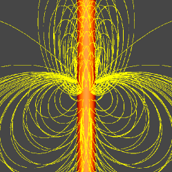
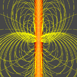
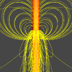
Figure 1: Three different viewing angles ($\phi=0$, $\phi=2\pi/3$ and $\phi=4\pi/3$) of a 3D plot of selected field lines for the example solution for $\xi(\varpi)=\xi_{0}=3/4$ and the dipole parameters $\varpi_{d}=0.5$, $\Theta=\pi/4$ and $\Psi=\pi/4$.

The pressure (normalised to $B_{0}^{2}/(2\mu_{0})=(\mu_{0}m^{2})/(2\pi^{2}R^{6})$) is given by

$$p(\varpi,\phi,z) = \bar{p}_{0}(\varpi)$$ (48)

$$\mbox{}-12\frac{[3D(\varpi-\varpi_{d}\cos(2\phi))-\sin\Theta(\cos\Psi\cos(2\phi)+\sin\Psi\sin(2\phi))r^{2}]^{2}}{r^{10}},$$

and the density is given by

$$\rho(\varpi,\phi,z)=\frac{1}{2\varpi}\left[\frac{{\rm d}\bar{p}_{0}}{{\rm d}\varpi}-\frac{3}{2}\mathbf{B}\cdot\nabla B_{\varpi}\right],$$ (49)

with the density normalised by $\mu_{0}m^{2}/(\pi^{2}\Omega R^{8})$. We have refrained from giving the explicit expression for the second term in the density as it is quite lengthy, but not really contributing to any better understanding of the problem. We are still free to specify a hydrostatic background plasma to complete our example. In Figure 2 we show contour plots in the $\phi$-$z$-plane for $\varpi=1.5$ and $\varpi=3.0$ of the logarithm of the pressure and the density. The background terms have been subtracted to emphasize the variation of pressure and density in $\phi$ and $z$. It turns out that for the two radii shown, the pressure term is always negative and we therefore show contours of the natural logarithm of its modulus, whereas the density term is positive. This means that the plasma pressure will be reduced compared to whatever background pressure is chosen, whereas the plasma density will be enhanced above the background plasma density.

Figure 2: Contour plots in the $\phi$-$z$ plane at radii $\varpi=1.5$ (top row) and $\varpi=3.0$ (bottom row) of the natural logarithm of the pressure and the density variation. Note that the background quantities have been subtracted as they can be chosen independently and only the three-dimensional terms are shown.

One can also see the strong radial decrease of the density term by comparing the values of the contours at $\varpi=1.5$ and $\varpi=3$. This is consistent with (49) which shows that the density term should have a $\varpi^{-8}$-dependence, whereas the pressure term has a $\varpi^{-6}$ variation (see (48)). Although the full expressions for the density and pressure will depend on the background model, this will usually mean that the three-dimensional variations of pressure and density will only be of importance close to the central cylinder and decrease fast with distance from the rotation axis ($\varpi$).

4 Summary and Discussion

Following Low (1991) we have presented a relatively simple analytical approach to calculate three-dimensional analytical MHD equilibria of rigidly rotating magnetospheres in cylindrical geometry. The fundamental equation that has to be solved is a linear second order PDE for a pseudo-potential $U$. The theory contains a free function $\kappa(V)$, or alternatively a function $\xi(\varpi)$, which can be chosen such that analytical progress is possible. Using the standard method of separation of variables, analytical solutions have been found for two different choices of $\xi(\varpi)$. For the choice of $\xi(\varpi)=\xi_{0}$ constant, one can also find solutions using a coordinate transformation method. We have used this method to find and discuss some illustrative solutions.

The solutions found here do not represent a complete model of the closed field line regions of rotating magnetospheres, because such a model would include the calculation of the free boundaries between open and closed field line regions and/or the boundaries between the closed field line regions and the plasma in which the magnetosphere is embedded. Determining the free boundaries generally involves matching the total pressure on both sides of the free boundary and obviously the choice of the hydrostatic background plasma, which is part of the set of solutions presented here will be important. Generally, if one would attempt to calculate a model with free boundaries using the results presented in this paper the separation of variable method is better suited than the transformation method due to the availability of a complete set of functions allowing the expansion of the general solution. The difficulty would be the nonlinear nature of the boundary conditions on and the unknown shape of the free boundary.

Possible modifications and extensions of the theory are to use spherical inner and outer boundaries or to use a combination of centrifugal and gravitational potential. This could, for example, be used to model the closed field line regions of fast rotating stars (see e.g. Ryan et al., 2005). In cylindrical geometry the modelling process will be very similar to that presented in the present paper, but with the additional complication that the combined potential

$$V(\varpi)=-\frac{1}{2}\Omega^{2}\varpi^{2}+2GM\ln(\varpi/R)$$ (50)

is not monotonic and thus cannot be mapped one-to-one to $\varpi$, because the combined potential has a maximum at the co-rotation radius $\varpi_{c}$, where the Kepler velocity equals the rotational velocity $\Omega\varpi_{c}$. A simple combination of $\kappa(V){V^{\prime}}^{2}$ into a function $\xi(\varpi)$ will usually lead to singularities in pressure and density at the co-rotation radius. Numerical solutions for physically sensible choices of $\kappa(V)$ are, however, possible in both cylindrical and spherical geometry and will be the subject of a future publication.

References

- Abramowitz and Stegun (1965) Abramowitz, M., and Stegun, I.A., Handbook of Mathematical Functions, New York: Dover Publications (1965).
- Bogdan and Low (1986) Bogdan, T.J., and Low, B.C. (1986), “The three-dimensional structure of magnetostatic atmospheres. II - Modeling the large-scale corona,” Astrophysical Journal, 306, 271–283.
- Ferraro (1937) Ferraro, V.C.A. (1937), “The non-uniform rotation of the Sun and its magnetic field,” Monthly Notices of the Royal Astronomical Society, 97, 458–472 4.
- Gibson and Bagenal (1995) Gibson, S.E., and Bagenal, F. (1995), “Large-scale magnetic field and density distribution in the solar minimum corona,” jgr, 100, 19865–19880.
- Gibson et al. (1996) Gibson, S.E., Bagenal, F., and Low, B.C. (1996), “Current sheets in the solar minimum corona,” Journal of Geophysical Research, 101, 4813–4824.
- Lanza (2008) Lanza, A.F. (2008), “Hot Jupiters and stellar magnetic activity,” Astronomy and Astrophysics, 487, 1163–1170.
- Low (1985) Low, B.C. (1985), “Three-dimensional structures of magnetostatic atmospheres. I - Theory,” Astrophysical Journal, 293, 31–43.
- Low (1991) Low, B.C. (1991), “Three-dimensional structures of magnetostatic atmospheres. III - A general formulation,” Astrophysical Journal, 370, 427–434.
- Low (1992) Low, B.C. (1992), “Three-dimensional structures of magnetostatic atmospheres. IV - Magnetic structures over a solar active region,” Astrophysical Journal, 399, 300–312.
- Low (1993a) Low, B.C. (1993a), “Three-dimensional structures of magnetostatic atmospheres. V - Coupled electric current systems,” Astrophysical Journal, 408, 689–692.
- Low (1993b) Low, B.C. (1993b), “Three-dimensional structures of magnetostatic atmospheres. VI - Examples of coupled electric current systems,” Astrophysical Journal, 408, 693–706.
- Mestel (1999) Mestel, L., Stellar Magnetism, Oxford: Clarendon Press (1999).
- Neukirch (1995) Neukirch, T. (1995), “On self-consistent three-dimensional solutions of the magnetohydrostatic equations,” Astronomy and Astrophysics, 301, 628–640.
- Neukirch (1997) Neukirch, T. (1997), “Nonlinear self-consistent three-dimensional arcade-like solutions of the magnetohydrostatic equations,” Astronomy and Astrophysics, 325, 847–856.
- Neukirch and Rastätter (1999) Neukirch, T., and Rastätter, L. (1999), “A new method for calculating a special class of self-consistent three-dimensional magnetoshydrostatic equilibria,” Astronomy and Astrophysics, 348, 1000–1004.
- Osherovich (1985a) Osherovich, V.A. (1985a), “Quasi-potential magnetic fields in stellar atmospheres. I - Static model of magnetic granulation,” Astrophysical Journal, 298, 235–239.
- Osherovich (1985b) Osherovich, V.A. (1985b), “The eigenvalue approach in modelling solar magnetic structures,” Australian Journal of Physics, 38, 975–980.
- Petrie and Neukirch (2000) Petrie, G.J.D., and Neukirch, T. (2000), “The Green’s function method for non-force-free three-dimensional solutions of the magnetohydrostatic equations,” Astronomy and Astrophysics, 356, 735–746.
- Ruan et al. (2008) Ruan, P., Wiegelmann, T., Inhester, B., Neukirch, T., Solanki, S.K., and Feng, L. (2008), “A first step in reconstructing the solar corona self-consistently with a magnetohydrostatic model during solar activity minimum,” Astronomy and Astrophysics, 481, 827–834.
- Rudenko (2001) Rudenko, G.V. (2001), “A constructing method for a self-consistent three-dimensional solution of the magnetohydrostatic equations using full-disk magnetogram data,” Solar Physics, 198, 279–287.
- Ryan et al. (2005) Ryan, R.D., Neukirch, T., and Jardine, M. (2005), “A simple model for the saturation of coronal X-ray emission of rapidly rotating late-type stars,” Astronomy and Astrophysics, 433, 323–334.
- Zhao and Hoeksema (1993) Zhao, X., and Hoeksema, J.T. (1993), “Unique determination of model coronal magnetic fields using photospheric observations,” Solar Physics, 143, 41–48.
- Zhao and Hoeksema (1994) Zhao, X., and Hoeksema, J.T. (1994), “A coronal magnetic field model with horizontal volume and sheet currents,” Solar Physics, 151, 91–105.
- Zhao et al. (2000) Zhao, X.P., Hoeksema, J.T., and Scherrer, P.H. (2000), “Modeling the 1994 April 14 Polar Crown SXR Arcade Using Three-Dimensional Magnetohydrostatic Equilibrium Solutions,” Astrophysical Journal, 538, 932–939.