The tangential map and associated integrable equations

Abstract

The tangential map is a map on the set of smooth planar curves. It satisfies the 3D-consistency property and is closely related to some well-known integrable equations.

1 Introduction

Let smooth planar curves $C$, $C_{1}$ and $C_{2}$ be given. Draw the tangent line to $C$ through any point $r$ on this curve, and let it meet $C_{1}$ in a point $r_{1}$ and $C_{2}$ in a point $r_{2}$. Let the tangent lines to the respective curves through these points meet in a point $r_{12}$. When the point $r$ moves along $C$, the point $r_{12}$ draws a new curve $C_{12}$. Thus, a local mapping on the set of planar curves is defined,

$$F:(C,C_{1},C_{2})\mapsto C_{12},$$

which will be referred to as the tangential map. The word “local” means that, first, the mapping is defined not for all triples of curves since the tangent to the curve $C$ may not intersect $C_{1}$ or $C_{2}$, and therefore only such curves or parts of the curves are considered where the construction is possible; second, the mapping may be multivalued since there may be several intersections, in this case a fixed branch of the mapping is considered.

Some properties of the tangential map are studied in this paper. It turns out to be rather simply related to the factorization of differential operators. In its turn, this allows to establish the relation with such integrable equations as semidiscrete ($\Delta\Delta D$) Toda lattice and, under a reduction, Hirota equation ($\Delta\Delta$). One of modifications of discrete KP equation ($\Delta\Delta\Delta$) appears in the discrete version of the tangential map. Thus, the tangential mapping is not a quite new object, rather it is of certain interest as one more geometric interpretation of well-known integrable equations.

2 3D-consistency

The main property of the tangential map is 3D-consistency. This means that if one starts from the curves $C,C_{1},C_{2},C_{3}$ and constructs the curves $C_{ij}=F(C,C_{i},C_{j})$ then the curve $C_{123}$ constructed from the triple $C_{i},C_{ij},C_{ik}$ is one and the same for any permutation of $i,j,k$. Alternatively, this can be formulated as follows.

Theorem 1.

The tangential map satisfies the (local) identity

$$C_{123} =F(C_{1},F(C,C_{1},C_{2}),F(C,C_{1},C_{3}))$$ (1)

$$=F(C_{2},F(C,C_{1},C_{2}),F(C,C_{2},C_{3}))$$

$$=F(C_{3},F(C,C_{1},C_{3}),F(C,C_{2},C_{3})).$$

The proof is given in the next Section. The combinatorial structure of identity (1) is represented by assigning the arguments of the mapping (the curves in our case) to the vertices of a cube, and the mapping itself to the faces, as shown on Fig. 1. The $N$-fold iteration of the mapping is associated with an $(N+1)$-dimensional cube.

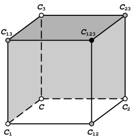
Figure 1: 3D-consistency, or consistency around a cube. The white vertices correspond to the given curves, the shaded faces show one of three possible construction ways of the curve corresponding to the black vertex.

The notion of 3D-consistency was formulated in [1, 2] in connection to the discrete integrable equations of the difference KdV type (the fields in the vertices of the cube) or to the Yang-Baxter type mappings (the fields on the edges of the cube). Both types of equations appear as nonlinear superposition principle for Darboux-Bäcklund transformations and are two-dimensional: two discrete independent variables correspond to the shifts along the edges of an elementary square. In contrast, the case of the tangential map is related to a three-dimensional equation: in addition to the discrete variables a continuous one appears corresponding to a parameter along the curves. Another important distinction is the asymmetry of the tangential map: the roles of the involved curves are obviously different. In particular, the formulas from the next section make clear that the construction of $C_{ij}$ from $C$, $C_{i}$, $C_{j}$ is described by a differential rational mapping, while the construction, for instance, of $C_{j}$ from $C$, $C_{i}$, $C_{ij}$ requires an additional integration. This explains the choice of the set $C$, $C_{i}$, $C_{j}$, $C_{k},\dots$ as preferable initial data, rather that the sequence $C$, $C_{i}$, $C_{ij}$, $C_{ijk},\dots$, as it is usual in the standard formulation of Yang-Baxter mappings [3].

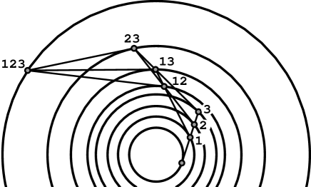
Figure 2: 3D-consistency of the tangential map in the simplest case of concentric circles

The simplest example illustrating the tangential map and its 3D-consistency property is given by the family of concentric circles (see Fig. 2), or, in slightly more general form, by the family of logarithmic spirals defined by equations $\rho_{i}=c_{i}e^{\gamma\varphi}$ in polar coordinates. The fact that the tangential map does not lead out of these families is clear from the invariance of the construction with respect to the rotations and scalings. However, the concurrence of the last three tangents is not spontaneously obvious (as an additional feature, in the case of family of circles, the points $r_{12},r_{13},r_{23}$ lie on the circle with $Or_{123}$ as diameter, where $O$ is the center of the family). Of course, this can be proved by elementary methods, but the point is that the concurrence of the tangents occurs in much more general situation. In Section 4.1 it will be demonstrated that this example corresponds to the simplest case of the factorization of differential operators with constant coefficients. Fig. 3 illustrates a nice property of the logarithmic spiral (in contrast to the previous plot, this one contains only three generations of points $r,r_{i},r_{ij}$, that is the triple intersections of the lines are not shown). This property can be formulated as the identity $F(C,C,C)=C$ for any branch of the map $F$.

Theorem 2.

Consider the intersection points of the logarithmic spiral with its tangent. The tangents through these points meet on the same spiral.

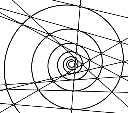
Figure 3: Jacob Bernoulli said “eadem mutata resurgo” on the logarithmic spiral; now in infinite number of ways

3 Factorization of differential operators

Let the curve $C$ be given in parametric form $r=r(t)$. Then the point of intersection with the curve $C_{i}$ is given, in the affine coordinates, by an equation of the form

$$r_{i}(t)=r(t)+a^{i}(t)\dot{r}(t),\qquad\dot{r}:=D(r):=\frac{dr}{dt}$$ (2)

with some coefficient $a^{i}$ (here and further on the subscript $i$ marks the quantities associated with the edge $CC_{i}$ of the combinatorial cube). This equation defines a parametrization of the curve $C_{i}$. It plays the role of an auxiliary linear problem for one branch of the tangential map. The curve $C_{ij}$ is defined from the compatibility condition

$$r_{ij} =r_{j}+a^{i}_{j}\dot{r}_{j}=r+a^{j}\dot{r}+a^{i}_{j}D(r+a^{j}\dot{r})$$

$$=r_{i}+a^{j}_{i}\dot{r}_{i}=r+a^{i}\dot{r}+a^{j}_{i}D(r+a^{i}\dot{r}),$$

where the coefficient $a^{i}_{j}$ correspond to the edge $C_{j}C_{ij}$.

Equating the coefficients for the linearly independent vectors $\dot{r},\ddot{r}$ yields the equations

$$a^{j}a^{i}_{j}=a^{i}a^{j}_{i},\quad(1+\dot{a}^{j})a^{i}_{j}+a^{j}=(1+\dot{a}^{i})a^{j}_{i}+a^{i}$$ (3)

which can be solved as the differential mapping $(a^{i},a^{j})\mapsto(a^{i}_{j},a^{j}_{i})$

$$a^{i}_{j}=\frac{(a^{i}-a^{j})a^{i}}{a^{i}-a^{j}+a^{i}\dot{a}^{j}-\dot{a}^{i}a^{j}}.$$ (4)

This is the formula which defines the action of the tangential map on the coefficients $a$. Alternatively, one can use the first of equations (3) in order to introduce the potential $v$ accordingly to the formula $a^{i}=v/v_{i}$, then the second equation rewrites as the differential mapping $f:(v,v_{i},v_{j})\mapsto v_{ij}$,

$$v_{ij}=\frac{v_{i}v_{j}}{v}+\frac{\dot{v}_{i}v_{j}-v_{i}\dot{v}_{j}}{v_{j}-v_{i}}.$$ (5)

The property of 3D-consistency is formulated in terms of the variables $a$ as the commutativity of the operators $T_{i}:a^{j}\to a^{j}_{i}$ which define the shift along the edges $CC_{i}$:

$$T_{i}T_{j}(a^{k})=T_{j}T_{i}(a^{k}),$$ (6)

and in terms of the variables $v$ as the identity of type (1):

$$v_{123} =f(v_{1},f(v,v_{1},v_{2}),f(v,v_{1},v_{3}))$$ (7)

$$=f(v_{2},f(v,v_{1},v_{2}),f(v,v_{2},v_{3}))$$

$$=f(v_{3},f(v,v_{1},v_{3}),f(v,v_{2},v_{3})).$$

Both identities can be proved straightforwardly, although the computation is rather tedious. It can be avoided by the following argument.

Proof of Theorem 1.

The above compatibility condition is equivalent to the equality

$$(1+a^{j}_{i}D)(1+a^{i}D)=(1+a^{i}_{j}D)(1+a^{j}D),$$ (8)

that is the definition of the tangential map amounts to the reconstruction of an ordinary second order differential operator from its kernel, under the condition of unitary constant term which is equivalent to affine normalization. Consider the differential operator

$$A=(1+T_{i}(a^{k}_{j})D)(1+a^{j}_{i}D)(1+a^{i}D)$$

corresponding to one of three possible ways of computing $r_{ijk}$. Accordingly to (8), $A$ is divisible from the right not only by $1+a^{i}D$, but also by $1+a^{j}D$. Moreover, two left factors of $A$ can be rewritten, again accordingly to (8), as $(1+T_{i}(a^{j}_{k})D)(1+a^{k}_{i}D)$, that is operator $A$ does not changes under permutation of $j$ and $k$. But this means that it is divisible from the right by $1+a^{k}D$ as well. Therefore, the kernel of $A$ is invariant with respect to any permutation of indices. Since a differential operator is uniquely defined by its kernel (up to a scalar factor which is fixed here by the condition that the constant term is unitary), hence the operator $A$ itself is invariant with respect to the permutations. ∎

Now it is clear that an $N$-fold tangential map corresponds to a differential operator of order $N$ divisible from the right by operators $1+a^{i}D$, $i=1,\dots,N$. This immediately leads to the Wronskian formula (for each of two components of $r$)

$$r_{1,2,\dots,N}=\frac{\det\begin{pmatrix}r&\varphi_{1}&\varphi_{2}&\dots&\varphi_{N}\\ \dot{r}&\dot{\varphi}_{1}&\dot{\varphi}_{2}&\dots&\dot{\varphi}_{N}\\ \vdots&\vdots&\vdots&&\vdots\\ D^{N}(r)&D^{N}(\varphi_{1})&D^{N}(\varphi_{2})&\dots&D^{N}(\varphi_{N})\end{pmatrix}}{\det\begin{pmatrix}\dot{\varphi}_{1}&\dot{\varphi}_{2}&\dots&\dot{\varphi}_{N}\\ \vdots&\vdots&&\vdots\\ D^{N}(\varphi_{1})&D^{N}(\varphi_{2})&\dots&D^{N}(\varphi_{N})\end{pmatrix}}$$

where $a^{i}=-\varphi_{i}/\dot{\varphi}_{i}$.

More simple mappings of type (4) and (5) are obtained from the factorization of operators normalized by the condition of unitary leading term:

$$(D-a^{j}_{i})(D-a_{i})=(D-a^{i}_{j})(D-a_{j}),$$

which is equivalent to

$$(T_{i}-1)(a^{j})=(T_{j}-1)(a^{i}),\quad\dot{a}^{i}-\dot{a}^{j}=a_{i}a^{j}_{i}-a^{j}a^{i}_{j},$$

and brings to the maps

$$a^{i}_{j}=a^{i}+\frac{\dot{a}^{i}-\dot{a}^{j}}{a^{i}-a^{j}}$$ (9)

and (under the substitution $a^{i}=v_{i}-v$)

$$v_{ij}=v_{i}+v_{j}-v+\frac{\dot{v}_{i}-\dot{v}_{j}}{v_{i}-v_{j}}$$ (10)

The 3D-consistency of these maps is proved analogously. Clearly, equations (4), (5) and (9), (10) are interpreted as 3-dimensional equations on $\mathbb{Z}^{2}\times\mathbb{R}$, with the fields $a$ corresponding to the edges of the lattice and $v$ corresponding to the vertices. These equations are related via simple substitutions to the semidiscrete Toda lattice, introduced in [4] for the first time (to the best of author’s knowledge), see also [5].

4 Examples and reductions

4.1 Logarithmic spirals

It is convenient to use the complex notation in this example, assuming $r=e^{(\gamma+{\rm i})t}$ (the case $\gamma=0$ correspond to the circle). Then $r_{k}=r+a^{k}\dot{r}=(1+\gamma a^{k}+{\rm i}a^{k})e^{(\gamma+{\rm i})t}$ and these curves are homothetic to the original one if and only if the coefficients $a^{k}$ are constant. The action of the map (4) on the constant coefficients is identical: $a^{k}_{j}=a^{k}$, therefore the tangential map amounts to the rotational dilation

$$r_{jk}=(1+\gamma a^{j}+{\rm i}a^{j})(1+\gamma a^{k}+{\rm i}a^{k})r$$

which preserves the family of curves under consideration. The $N$-fold mapping is given by analogous explicit formula, so that this example can be considered trivial. However, even this example demonstrates that the established relation between the tangential map and differential operators is not one-to-one and depends on the choice of initial curve and its parametrization. The mappings corresponding to the same operators (that is, with the same coefficients $a$) can be regarded as locally equivalent, but the global picture may be quite different. For example, the tangential map has four branches in the case of concentric circles (real if the radius of $C$ is less than the radii of $C_{1},C_{2}$) and infinite number of branches in the case of logarithmic spirals.

In order to obtain the auto-mapping shown on Fig. 3, one has to assume the additional constraint $r_{k}(t)=r(t+\delta_{k})$ (then $r_{jk}(t)=r(t+\delta_{j}+\delta_{k})$, $r_{jkl}(t)=r(t+\delta_{j}+\delta_{k}+\delta_{l})$ and so on), that is

$$e^{(\gamma+{\rm i})(t+\delta_{k})}=(1+\gamma a^{k}+{\rm i}a^{k})e^{(\gamma+{\rm i})t}.$$

This implies that $\delta_{k}$ are roots of the transcendental equation

$$\cos\delta-\gamma\sin\delta=\exp(-\gamma\delta),$$

and the coefficients $a^{k}$ are expressed by the formula

$$a^{k}=\exp(\gamma\delta_{k})\sin\delta_{k}.$$

It can be derived from here (this is left to the reader as an easy exercise), that the boundary of the domain free of the lines on Fig. 3 is approximated by a parabola. The numeric values for this plot are $\gamma=0.1$, $\delta_{1}=5.24$, $\delta_{2}=7.25,\dots$

4.2 Any curve

The previous example suggests that a picture with good global behavior of the curves can be obtained if the starting curve is the circle $r=e^{{\rm i}t}$ again, and the coefficients $a^{k}(t)$ are almost constant functions with periods commensurable with $\pi$. For instance, the left plot on Fig. 4 corresponds to

$$a^{1}=1+\frac{1}{5}\cos\frac{3}{2}t,\quad a^{2}=2+\frac{1}{10}\cos\Bigl{(}\frac{t}{2}+\frac{\pi}{4}\Bigr{)}.$$

The right plot corresponds to the choice

$$a^{1}=4+\sin t,\quad a^{2}=4+\cos t,$$

here the tangential map brings to the curve with cusps.

    

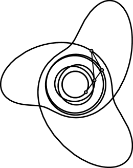
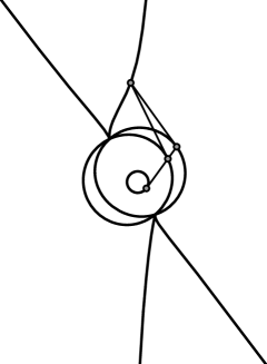
Figure 4: Examples of the tangential map

4.3 Loxodromes

We will say, slightly abusing the terminology, that a curve $\widetilde{C}$ is a loxodrome for a given curve $C$ if it intersects the tangents to $C$ under a constant angle $\gamma$ (in particular, if $\gamma=\pi/2$, then $\widetilde{C}$ is an involute of $C$).

Theorem 3 below demonstrates that the tangential map preserves this type of relation between the curves (see Fig. 5). As a preliminary, it is convenient to introduce the parameter on the curve $C$ accordingly to equations

$$\dot{r}=y(t)\tau,\quad\dot{\tau}=\nu,\quad\dot{\nu}=-\tau$$ (11)

where $\tau,\nu$ are unit tangent and normal vectors. Obviously, the function $y$ is the radius of curvature and the relation to the natural parametrization by arc length $r=r(s)$ is

$$y(t(s))=1/\kappa(s),\quad dt=\kappa(s)ds.$$

This choice of parametrization is explained by the fact that its form is preserved for the curve $\widetilde{C}$ as well. Indeed, the equation of a point on this curve is $\tilde{r}=r+a\dot{r}=r+ay\tau$. Then

$$\dot{\tilde{r}}=(y+D(ay))\tau+ay\nu$$

and since $\tilde{r}$ meets $\tau$ under the constant angle $\gamma$ (reckoned in the direction of the normal $\nu$, for definiteness), hence

$$y+D(ay)=ay\cot\gamma.$$ (12)

In virtue of this constraint, the equalities

$$\dot{\tilde{r}}=\tilde{y}\tilde{\tau},\quad\dot{\tilde{\tau}}=\tilde{\nu},\quad\dot{\tilde{\nu}}=-\tilde{\tau}$$

hold, with

$$\tilde{y}=\frac{ay}{\sin\gamma},\quad\tilde{\tau}=\tau\cos\gamma+\nu\sin\gamma,\quad\tilde{\nu}=\nu\cos\gamma-\tau\sin\gamma.$$

Thus, we have proved that the choice of $t$ as the parameter brings to equations of the type (11) for the loxodrome $\widetilde{C}$ as well. If the function $y$ is given then the constraint (12) is the determining equation for the coefficient $a$, and the loxodrome is constructed by any solution of it.

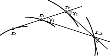
Figure 5: Loxodromic reduction of the tangential map

Theorem 3.

Let curves $C_{i}$ and $C_{j}$ meet tangents to a curve $C$ under constant angles $\gamma^{i}$ and $\gamma^{j}$ respectively, and $\gamma^{i}\neq\gamma^{j}$. Then the curve $C_{ij}=F(C,C_{i},C_{j})$ meets tangents to $C_{i}$ under the angle $\gamma^{j}$ and tangents to $C_{j}$ under the angle $\gamma^{i}$.

Proof.

Assume the parametrization (11) for the curve $C$. Then, as it was shown before, the parameters $a^{k}$ of the tangential map and the functions $y_{k}$ for the loxodromes are related by

$$y+D(a^{k}y)=a^{k}y\cot\gamma^{k},\quad y_{k}=\frac{a^{k}y}{\sin\gamma^{k}},\quad k=i,j.$$

It is easy to prove that in virtue of these constraints the tangential map (4) takes the form

$$a^{i}_{j}=\frac{a^{i}/a^{j}-1}{\cot\gamma^{j}-\cot\gamma^{i}}$$

and moreover, the identity

$$y_{j}+D(a^{i}_{j}y_{j})=a^{i}_{j}y_{j}\cot\gamma^{i}$$

holds, which is the constraint of the form (12) for the functions $y_{j}$ and $a^{i}_{j}$. But this means exactly that the curve $C_{ij}$ is a loxodrome for $C_{j}$, corresponding to the angle $\gamma^{i}$. ∎

Formally, this statement looks like well-known Bianchi theorem on the permutability of Darboux-Bäcklund type transformations (see Fig. 6). However, it is clear from the proof that in our case the situation is more simple: indeed, Bäcklund transformations amount to solving of Riccati equations, while the construction of the loxodromes amounts, accordingly to (12), to a simple quadrature. The superposition principle for the transformations under consideration turns out to be linear:

$$\sin(\gamma^{i}-\gamma^{j})y_{ij}=\sin(\gamma^{i})y_{i}-\sin(\gamma^{j})y_{j}.$$

A genuine Darboux transformation leading to the nonlinear superposition principle is provided by the reduction presented in the next example.

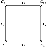
Figure 6: Bianchi diagram

4.4 Darboux transformation

Let $H_{\gamma}$ be the homothety with a coefficient $\gamma\neq 1$ with respect to a fixed point (origin) in the plane. We will say that the curves $C$, $\widetilde{C}$ are in the tangential correspondence with parameter $\gamma$ if the tangent to the curve $C$ through any point $r$ meets $H_{\gamma}(\widetilde{C})$ in the point $H_{\gamma}(\tilde{r})$, and the tangent to $\widetilde{C}$ through $\tilde{r}$ meets $H_{\gamma}(C)$ in the point $H_{\gamma}(r)$ (see Fig. 7).

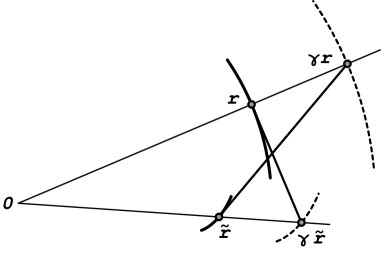
Figure 7: Tangential correspondence

As in the example with the loxodromes, this notion defines some reduction of the tangential map which can be studied more conveniently in some special parametrization of the curves. The points on the curves $C$, $\widetilde{C}$ are related by equations of the form

$$\gamma\tilde{r}(t)=r(t)+a(t)\dot{r}(t),\quad\gamma r(t)=\tilde{r}(t)+b(t)\dot{\tilde{r}}(t),$$

which imply that the vector-functions $r(t),\tilde{r}(t)$ satisfy linear second order ODEs

$$ab\ddot{r}+(\dot{a}b+a+b)\dot{r}+(1-\gamma^{2})r=0,$$

$$ab\ddot{\tilde{r}}+(a\dot{b}+a+b)\dot{\tilde{r}}+(1-\gamma^{2})\tilde{r}=0.$$

Therefore, the ratio of the first and the last coefficients is the same for $r$ and $\tilde{r}$, that is it is an invariant of the tangential correspondence. It is convenient to use such a parametrization that this ratio is constant. Let

$$\lambda ab=1-\gamma^{2},\quad\lambda=(1-\gamma^{2})\mu,$$

then the equations take the form

$$\ddot{r}+u\dot{r}+\lambda r=0,\quad\ddot{\tilde{r}}+\tilde{u}\dot{\tilde{r}}+\lambda\tilde{r}=0$$ (13)

where functions $u,\tilde{u}$ are related to the coefficient $a$ via the pair of Riccati equations

$$\dot{a}+1-ua+\mu a^{2}=0,\quad-\dot{a}+1-\tilde{u}a+\mu a^{2}=0.$$

The first one is linearized by the substitution $a=-\phi/\dot{\phi}$ which brings to equation $\ddot{\phi}+u\dot{\phi}+\mu\phi=0$. Thus, the curve $\widetilde{C}$ is constructed by use of a particular scalar solution of the differential equation for the original curve $C$, at the value of the parameter $\lambda=\mu$, that is the tangential correspondence is nothing but an example of Darboux transformation.

Theorem 4.

Let a curve $C$ be in the tangential correspondence with curves $C_{i}$, $C_{j}$, with parameters $\gamma^{i}$, $\gamma^{j}$ respectively, and $\gamma^{i}\neq\gamma^{j}$. Then an unique curve $C_{ij}$ exists which is in the tangential correspondence with the curves $C_{i}$, $C_{j}$, with the parameters $\gamma^{j}$, $\gamma^{i}$ respectively. Moreover,

$$H_{\gamma^{i}\gamma^{j}}(C_{ij})=F(C,H_{\gamma^{i}}(C_{i}),H_{\gamma^{j}}(C_{j})).$$

Proof.

It follows directly from the definitions of the tangential map and the tangential correspondence that if such a curve $C_{ij}$ exists then it is unique and is given by the above formula. So we only need to verify that this curve is indeed in the tangential correspondence with $C_{i}$, $C_{j}$, by use of the relations

$$\dot{a}^{k}+1=ua^{k}-\mu^{k}(a^{k})^{2},\quad u_{k}=-u+2\mu^{k}a^{k}+\frac{2}{a^{k}},\quad k=i,j.$$

It is easy to prove that the formula (4) takes, in virtue of these constraints, the algebraic form

$$a^{i}_{j}=\frac{a^{i}-a^{j}}{a^{j}(\mu^{i}a^{i}-\mu^{j}a^{j})},$$ (14)

and that the coefficient $A=a^{i}_{j}$ identically satisfies the Riccati equation

$$\dot{A}+1-u_{j}A+\mu^{i}A^{2}=0.$$

This means that the curves $C_{ij}$, $C_{j}$ are in tangential correspondence, with parameter $\gamma^{i}$. ∎

It should be noticed that equation (13) for $r$ defines the spectral problem for the $\sinh$-Gordon equation, mapping (14) is equivalent to the mapping ($F_{4}$) from [6], and the substitution $a^{i}=v/v_{i}$, $u=2\dot{v}/v$ brings to the equation

$$v_{ij}(v_{j}-v_{i})=v(\mu_{i}v_{j}-\mu_{j}v_{i})$$

which is equivalent to the Hirota equation [7].

Analogously, the mapping (9) admits the similar reduction

$$\dot{a}^{k}=u+\gamma^{k}-(a^{k})^{2},\quad u_{k}=-u-2\gamma^{k}+2(a^{k})^{2}$$

which brings to the mapping

$$a^{i}_{j}=-a^{j}+\frac{\gamma^{i}-\gamma^{j}}{a^{i}-a^{j}}.$$

This is one of the forms of nonlinear superposition principle of Darboux transformation for the Shrödinger operator [8].

5 Further generalizations

5.1 Discrete tangential map

Let us consider discrete curves $r=r(n)$, then an analog of equation (2) reads

$$r_{i}=r+a^{i}(T-1)(r),\quad T:n\mapsto n+1.$$

The compatibility condition of such equations

$$r_{ij} =(1+a^{i}_{j}(T-1))(1+a^{j}(T-1))(r)$$

$$=(1+a^{j}_{i}(T-1))(1+a^{i}(T-1))(r).$$

brings to the relations

$$T(a^{j})a^{i}_{j}=T(a^{i})a^{j}_{i},\quad(1-a^{j})a^{i}_{j}+a^{j}=(1-a^{i})a^{j}_{i}+a^{i},$$

which yield a discrete analog of tangential map (4):

$$T_{j}(a^{i})=a^{i}_{j}=\frac{(a^{i}-a^{j})T(a^{i})}{(1-a^{j})T(a^{i})-(1-a^{i})T(a^{j})}.$$ (15)

The substitution $a^{i}=T(v)/v_{i}$ brings to an analog of map (5):

$$f:(v,v_{i},v_{j})\mapsto v_{ij}=\frac{v_{i}v_{j}T(v_{j}-v_{i})}{T(v)(v_{j}-v_{i})}+\frac{T(v_{i})v_{j}-v_{i}T(v_{j})}{v_{j}-v_{i}}.$$ (16)

The symmetric form of this equation

$$\frac{T(v_{j}-v_{i})}{T(v)}+\frac{T(v_{i})-v_{ij}}{v_{i}}+\frac{v_{ij}-T(v_{j})}{v_{j}}=0,$$

demonstrates that the shift $T$ is actually on the equal footing with $T_{i}$ and $T_{j}$. Difference substitutions relate this equation to the discrete Toda and KP equations (in particular, the variable $v$ is identified as the wave function of the linear problem for KP equation [9]). Alternative geometric interpretations of these equations can be found in the papers [10, 9], see also [11] where a general theory of this class of equations is developed.

The 3D-consistency property of the maps (15) and (16) is formulated by the same general identities (6), (7) as in the continuous case, and is proved along the lines of the proof of Theorem 1. There exist also the simple geometric explanation of this property: the triangles $r_{12}(n)r_{13}(n)r_{23}(n)$ and $r_{12}(n+1)r_{13}(n+1)r_{23}(n+1)$ are perspective with respect to the line $r(n+1)r(n+2)$ (marked by $n+1$ on Fig. 8), therefore, accordingly to Desargues theorem, the lines $r_{12}(n)r_{12}(n+1)$, $r_{13}(n)r_{13}(n+1)$ and $r_{23}(n)r_{23}(n+1)$ are concurrent, as required.

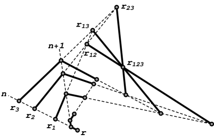
Figure 8: 3D-consistency of the discrete tangential map

5.2 The higher order maps

Equation (2) can be replaced by

$$r_{i}(t)=r(t)+a^{1,i}(t)\dot{r}(t)+\dots+a^{m,i}(t)D^{m}(r(t)),$$

for the curves in a space of dimension greater or equal to $2m$. In the discrete case one has analogously

$$r_{i}(n)=r(n)+a^{1,i}(n)(r(n+1)-r(n))+\dots+a^{m,i}(n)(r(n+m)-r(n)).$$

It is not difficult to demonstrate that the compatibility condition $T_{j}T_{i}(r)=T_{i}T_{j}(r)$ is equivalent to a system of $2m$ equations which can be solved in the form of differential or difference mapping

$$(a^{1,i},\dots,a^{m,i},a^{1,j},\dots,a^{m,j})\mapsto(a^{1,i}_{j},\dots,a^{m,i}_{j},a^{1,j}_{i},\dots,a^{m,j}_{i}),$$

with the derivatives or shifts up to $m$-th order. These mappings are 3D-consistent, which can be proved by arguments analogous to the case $m=1$ just considered. Unfortunately, the explicit form of these mappings is too bulky already at $m=2$, so it would be desirable to find some reduction lowering their order and/or number of fields.

Acknowledgements.

This work was supported by RFBR grants 08-01-00453 and SS-3472.2008.2.

References

- [1] F.W. Nijhoff, A.J. Walker. The discrete and continuous Painlevé hierarchy and the Garnier system. Glasgow Math. J. 43A (2001) 109–123.
- [2] A.I. Bobenko, Yu.B. Suris. Integrable systems on quad-graphs. Int. Math. Res. Notes (2002) 573–611.
- [3] A.P. Veselov. Yang-Baxter maps and integrable dynamics. Phys. Lett. A 314:3 (2003) 214–221.
- [4] D. Levi, L. Pilloni, P.M. Santini. Integrable three-dimensional lattices. J. Phys. A 14:7 (1981) 1567–1575.
- [5] V.E. Adler, S.Ya. Startsev. Discrete analogues of the Liouville equation. Theor. Math. Phys. 121:2 (1999) 271–284.
- [6] V.E. Adler, A.I. Bobenko, Yu.B. Suris. Geometry of Yang-Baxter maps: pencils of conics and quadrirational mappings. Comm. Anal. and Geom. 12:5 (2004) 967–1007.
- [7] R. Hirota. Nonlinear partial difference equations. III. Discrete sine-Gordon equation.J. Phys. Soc. Japan 43 (1977) 2079–2086.
- [8] A.P. Veselov, A.B. Shabat. Dressing chain and the spectral theory of Schrödinger operators. Funct. Anal. Appl. 27:2 (1993) 10–30.
- [9] B.G. Konopelchenko, W.K. Schief. Menelaus’ theorem, Clifford configurations and inversive geometry of the Schwarzian KP hierarchy. J. Phys. A 35:29 (2002) 6125–6144.
- [10] A. Doliwa. Geometric discretization of the Toda system. Phys. Lett. A 234 (1997) 187–192.
- [11] V.E. Adler, A.I. Bobenko, Yu.B. Suris. The classification of integrable discrete equations of octahedron type, to appear, 2009.