CARS: The CFHTLS-Archive-Research Survey
III. First detection of cosmic magnification in samples of normal high-$z$ galaxies

Abstract

Context. Weak gravitational lensing (WL) has been established as one of the most promising probes of cosmology. So far, most studies have exploited the shear effect of WL leading to coherent distortions of galaxy shapes. WL also introduces coherent magnifications.

Aims. We want to detect this cosmic magnification effect (coherent magnification by the large-scale structure of the Universe) in large samples of high-redshift galaxies selected from the Deep part of the Canada-France-Hawaii-Telescope Legacy Survey (CFHTLS).

Methods. Lyman-break galaxies (LBGs) selected by their colours to be at $z$=2.5-5, are used as a background sample and are cross-correlated to foreground lens galaxies, which are selected by accurate photometric redshifts (photo-$z$’s). The signals of LBGs in different magnitude bins are compared to predictions from WL theory. An optimally weighted correlation function is estimated by taking into account the slope of external LBG luminosity functions.

Results. For the first time, we detect cosmic magnification in a sample of normal galaxies. These background sources are also the ones with the highest redshifts so far used for WL measurements. The amplitude and angular dependence of the cross-correlation functions agree well with theoretical expectations and the lensing signal is detected with high significance. Avoiding low-redshift ranges in the foreground samples which might contaminate the LBG samples we can make a measurement that is virtually free of systematics. In particular, we detect an anti-correlation between faint LBGs and foreground galaxies which cannot be caused by redshift overlap.

Conclusions. Cross-correlating LBGs (and in future also photo-$z$ selected galaxies) as background sources to well understood foreground samples based on accurate photo-$z$’s will become a powerful cosmological probe in future large imaging surveys.

1 Introduction

Many studies have shown so far that images of faint background galaxies are coherently distorted by the gravitational lensing effect of the large-scale structure in the line of sight. This cosmic shear effect (Munshi et al., 2008; Hoekstra & Jain, 2008, for recent reviews see) has been identified to be one of the most promising approaches to study the properties of dark matter and dark energy (Albrecht et al., 2006; Peacock et al., 2006). It relies on the assumption that the ellipticities of background galaxies are intrinsically randomly distributed. Cosmic shear introduces tiny, coherent distortions to this random distribution, which can be measured (see e.g. Benjamin et al., 2007; Fu et al., 2008).

Besides this shear effect of gravitational lensing the images of background galaxies are also subject to magnification by the large-scale structure of the Universe. However, no simple assumption about the intrinsic distribution of the fluxes of the background galaxies can be made. Rather, this distribution has to be measured from the data by averaging over large areas of the sky.

The magnification effect of gravitational lensing to first order depends on the convergence only, which is the projected mass along the line-of-sight. This effect is geometrical in nature enlarging the solid angle behind masses. This leads to two distinct effects, a dilution of the source density and a magnification of their fluxes since lensing conserves the surface brightness. Now it depends on the intrinsic distribution of the fluxes whether the angular sky positions of the background galaxies of a given observed flux are positively or negatively cross-correlated to the angular positions of the foreground masses. If there are many more faint background galaxies than bright ones, i.e. steep magnitude number counts, the magnification wins over the dilution and a positive angular cross-correlation is expected. In the case of shallow number counts the dilution becomes dominant and a negative angular cross-correlation is expected. This general effect of gravitational lensing is called magnification bias and in the case of the large-scale structure of the Universe as the lens it is referred to as cosmic magnification.

Measurements of the cosmic magnification signal can be interpreted in a similar way as signals of galaxy-galaxy lensing (see e.g. Brainerd et al., 1996; Hoekstra et al., 2004; Mandelbaum et al., 2006; Parker et al., 2007). Thus, cosmic magnification can be directly employed to study the dark matter environment of galaxies constraining the galaxy bias, the total matter density, and the normalisation of the dark matter power spectrum.

The biggest problem in using magnification as a cosmological probe is to cleanly separate the fore- and the background samples in redshift. If there is some redshift overlap between the samples - i.e. if the lens and source galaxies are physically close - they see the same dark matter field and will hence cluster with respect to each other. Then the angular cross-correlation signal is not a pure lensing signal anymore but it is contaminated by physical cross-correlations.

Due to this complication the effect has only been convincingly measured with high significance in the Sloan Digital Sky Survey (SDSS) by Scranton et al. (2005) using optically selected quasars as background sources (see also Ménard et al., 2009, for a different estimator of the cosmic magnification signal with the same data). For the long and controversial history of such measurements of quasar-galaxy cross-correlation we refer the reader to the references within that paper.

Here we present the first measurement of the same effect on normal galaxies which have a much higher surface density on the sky than quasars and can thus lead to much more accurate results. The Lyman-break technique allows for the selection of clean samples of high-redshift star-forming galaxies from optical data. In Hildebrandt et al. (2009) we presented the largest survey of these galaxies to date. More than 80 000 LBG candidates with redshifts $z=2.5-5$ were selected from the data of the Deep part of the CFHTLS and their clustering properties were measured. The same samples are used here to detect cosmic magnification by cross-correlating them to foreground galaxies.

In Sect. 2 we review the theoretical framework which is necessary to interpret the measurements. The data analysis is covered in Sect. 3 and the results are presented in Sect. 4. Conclusions and an outlook to future applications of this method are given in Sect. 5. Throughout the paper we assume $H_{0}=70\frac{\rm km}{\rm s\,Mpc}$, $\Omega_{\rm m}=0.3$, $\Omega_{\Lambda}=0.7$, and $\sigma_{8}=0.8$, and we use AB magnitudes.

2 Theoretical framework

Let $N_{0}(>f)$ be the unlensed cumulative number counts of background galaxies with fluxes larger than $f$. For simplicity we assume that all background galaxies are at the same redshift. Foreground structures will lead to a magnification $\mu$ at a particular position on the sky. The lensed cumulative number counts are related to the unlensed ones in the following way (Bartelmann & Schneider, 2001):

$$N(>f)=\mu^{-1}\,N_{0}(>\mu^{-1}f)\,,$$ (1)

where the first $\mu$ corresponds to the dilution of the sample due to the enlargement of the solid angle behind the lens and the second $\mu$ corresponds to the brightening due to the enlargement of the sources.

We assume that $N_{0}(f)$ can be approximated by a power-law:

$$N_{0}(>f)=A\,f^{-\alpha}\,,$$ (2)

with $A$ being the amplitude and $\alpha$ being the slope of the power-law. The lensed cumulative number counts then become:

$$N(>f)=\mu^{\alpha-1}N_{0}(>f)\,,$$ (3)

Thus, it depends on the slope $\alpha$ of $N_{0}(>f)$ whether the surface density of background sources is increased or decreased near lenses where $\mu>1$. In the weak-lensing regime $\mu$ is close to unity so that we can write $\mu=1+\delta\mu$ with $\delta\mu\ll 1$ and a Taylor expansion yields

$$\mu^{\alpha-1}\approx 1+(\alpha-1)\delta\mu\,.$$ (4)

Using magnitudes instead of fluxes (i.e. substituting $m=-2.5\log(f)+{\rm const.}$) it can easily be shown that $\alpha$ is related to the differential magnitude numbercounts:

$$2.5\frac{\mathrm{d}\log n(m)}{\mathrm{d}m}=\alpha\,,$$ (5)

with $n(m)$ being the number counts of galaxies with magnitudes in the interval $[m,m+\mathrm{d}m]$. By measuring the logarithmic slope of the magnitude number counts we can predict over- or under-densities of background galaxies induced by lensing.

Under the assumption of a linear biasing factor $b$ for the foreground galaxies, the angular cross-correlation between these foreground lenses and the background sources, $w_{\rm sl}(\theta)$, is related to the angular cross-correlation between magnification and matter density contrast, $w_{\mu\delta}(\theta)$ by:

$$w_{\rm sl}(\theta)=(\alpha-1)\,b\,w_{\mu\delta}(\theta)\,.$$ (6)

For this result we employed Eqs. 3 & 4, the definition of the cross-correlation function, and the assumption of a linear relation between matter- and galaxy-density.

We calculate $w_{\mu\delta}(\theta)$ as described in Bartelmann & Schneider (2001):

$$w_{\mu\delta}(\theta)=\frac{3H_{0}^{2}\,\Omega_{\rm m}}{c^{2}}\int_{0}^{\chi_{\rm H}}\mathrm{d}\chi^{\prime}\,f_{K}(\chi)\,W_{\rm s}(\chi^{\prime})\,G_{\rm l}(\chi^{\prime})\,a^{-1}(\chi^{\prime})\>\times\\ \int_{0}^{\infty}\frac{k\,\mathrm{d}k}{2\pi}\,P_{\delta}(k,\chi^{\prime})\,J_{0}[f_{K}(\chi^{\prime})\,k\,\theta]\,,$$ (7)

with $\chi$ being the comoving distance, $f_{K}$ being the comoving angular diameter distance, $W_{\rm s}(\chi)=\int_{\chi}^{\chi_{\rm H}}\mathrm{d}\chi^{\prime}G_{\rm s}(\chi^{\prime})\frac{f_{K}(\chi^{\prime}-\chi)}{f_{K}(\chi^{\prime})}$ being the weight function of the sources, $G_{\rm l/s}$ being the normalised distance distribution of the lenses/sources, $a$ being the scale factor, $P_{\delta}$ being the matter power spectrum, and $J_{0}$ being the 0th-order Bessel function of the first kind.

In order to measure the signal of Eq. 6 from data it is of utmost importance to cleanly separate the sources from the lenses. Otherwise physical cross-correlations will swamp the tiny signal and make an interpretation in the framework of weak gravitational lensing impossible because these physical cross-correlation are typically larger than the cosmic magnification signal by an order of magnitude.

3 Data analysis

3.1 The dataset

The data used in this study are taken from the CFHTLS-Deep Survey, an imaging survey with MEGACAM@CFHT in the filters $ugriz$ in four independent fields of 1 square degree each. In the framework of the CARS (CFHTLS-Archive-Research Survey) project we have collected all publicly available data until July 21, 2008. The data reduction is carried out with the THELI imaging reduction pipeline (Erben et al., 2005) and is described in detail in Erben et al. (2009) and Hildebrandt et al. (2009).

Multi-colour catalogues are created with SExtractor (Bertin & Arnouts, 1996) in dual-image mode from images convolved to the same seeing. Photo-$z$’s for all objects are estimated with a modified version of the BPZ code (Benítez, 2000) including a correction for galactic extinction (with the maps of Schlegel et al., 1998), a re-calibration of the photometric zeropoints and the template set with the help of spectroscopic redshifts (see Capak, 2004), and a modified prior. For details on the catalogue creation see Hildebrandt et al. (2009).

3.2 The LBG catalogues

In Hildebrandt et al. (2009) we describe how we select large samples of LBGs from these data. Simulations are set up to identify regions in two-colour-space where high-redshift sources can be selected with high efficiency and low contamination. In this way we select $\sim 34\,000$ $u$-dropouts at $z\sim 3.2$, $\sim 36\,000$ $g$-dropouts at $z\sim 3.8$, and $\sim 10\,000$ $r$-dropouts at $z\sim 4.7$. The faintest LBGs that can be selected in that way from these data have measured total magnitudes of $r=27.6$, $i=27.8$, and $z=27.8$ for the $u$-, $g$-, and $r$-dropouts, respectively.

The simulated redshift distributions are displayed in Fig. 1. These suggest that the $u$-dropout sample is essentially free of any low-$z$ contamination , whereas the $g$-dropout sample is contaminated by a small fraction ($\sim 4\%$) of low-$z$ galaxies with redshifts $0<z<0.5$, and the $r$-dropout sample is contaminated very slightly ($\sim 2.5\%$) by galaxies with redshifts $0.5<z<1.0$. One of the big advantages of using LBGs as background sources is that we know the redshifts of the possible contaminants. In the remainder of the paper we try to avoid these redshift regions, which might be affected by some small amount of contamination, in our foreground lens samples in order not to mix the lensing signal with a signal from physical cross-correlations.

Figure 1: Simulated redshift distributions of the three dropout samples ($u$-dropouts: solid, $g$-dropouts: dotted, $r$-dropouts: dashed; arbitrarily normalised but with correct relative fractions). The simulations are based on templates from the library of Bruzual & Charlot (1993). See Hildebrandt et al. (2009) for a detailed description of the simulations.

For a given LBG background sample we approximate $G_{\rm s}$ of Eq. 7 by a Dirac delta-function at the mean redshift of the LBGs. This approximation is valid because the comoving distance - the quantity on which the lensing signal depends - does not change appreciably over the range where the LBG redshift distribution is different from zero, i.e. the distributions in comoving distance are very narrow for the LBGs (in contrast to the redshift distributions).

As described in Sect. 2, the amplitude of the cosmic magnification signal in the angular cross-correlation function of low- and high-$z$ galaxies depends on the slope of the number counts of the background sample. The number counts of the three samples and of the combined $u$&$g$-dropout sample are shown in Fig. 2. For fainter magnitudes incompleteness sets in. While this incompleteness does not bias the measurement of the cross-correlation function (to first order), it prevents a measurement of the slope of the number counts at the faint end, which is necessary to carry out the theoretical predictions.

Figure 2: Number counts of the three dropout samples and of the combined $u$&$g$-dropout sample.

However, the number counts are closely related to the luminosity function (LF). For a complete sample of galaxies in a thin redshift slice the two curves are related to each other in magnitude by the distance modulus and in amplitude by the volume normalisation. Thus, using an external LBG-LF that has been properly corrected for incompleteness one can predict the slope of the number counts. The volume normalisation does not play a role here since we are only interested in the slope.

The LBG-LF, $\Phi(M)$, was precisely measured in several studies at $z\sim 3$ (Steidel et al., 1999; Sawicki & Thompson, 2006), $z\sim 4$ (Steidel et al., 1999; Ouchi et al., 2004; Giavalisco et al., 2004; Sawicki & Thompson, 2006; Yoshida et al., 2006; Bouwens et al., 2007), and $z\sim 5$ (Iwata et al., 2003, 2007; Ouchi et al., 2004; Giavalisco et al., 2004; Yoshida et al., 2006). Assuming a Dirac delta-function for the redshift distribution of the LBGs, the slope of the number counts of a complete sample of LBGs equals the slope of the luminosity function. The parameter $\alpha$ introduced in Sect. 2 can thus be expressed as

$$\alpha(m)=2.5\,\mathrm{d}\log\mathrm{n}(m)/\mathrm{d}m=2.5\,\mathrm{d}\log\Phi(M)/\mathrm{d}M\,,$$ (8)

with $m=M+DM+K$ and $DM$ being the distance modulus and $K$ being the $K$-correction.

For the theoretical predictions we choose different LFs by Steidel et al. (1999), Sawicki & Thompson (2006), and Bouwens et al. (2007) spanning a range of faint-end slopes and parametrised in the way described by Schechter (1976):

$$\Phi(M)\mathrm{d}M=0.4\,\Phi^{*}\ln(10)\left[10^{0.4(M_{*}-M)}\right]^{\alpha_{\rm LF}+1}\\ \times\exp[-10^{0.4(M_{*}-M)}]\mathrm{d}M\,.$$ (9)

Note that $\alpha(m)$ of Eq. 8 approaches the value of the Schechter LF parameter $\alpha_{\rm LF}$ for faint magnitudes.

The Schechter function parameters of these external LFs are listed in Table 1. We fit our number counts with a fourth order polynomial in magnitude only for comparison to the external LFs and not for prediction of the magnification signal. In Fig. 3 we show the adopted values of $\alpha-1$ as a function of LBG magnitude for the different samples and the different LF measurements in the literature in comparison to the fitted polynomial. We use the $z\sim 4$ values of Steidel et al. (1999) and Sawicki & Thompson (2006) to estimate a $z\sim 5$ LF and the $z\sim 4$ values of Bouwens et al. (2007) to estimate the $z\sim 3$ LF assuming no evolution.

Table 1: Schechter (1976) function parameters for the external LFs

Reference	$M_{*}$	$\alpha_{\rm LF}$
$z\sim 3$
Steidel et al. (1999)	$-21.00$	$-1.60$
Sawicki & Thompson (2006)	$-20.90$	$-1.43$
Bouwens et al. (2007)	$-20.98$	$-1.73$
$z\sim 4$
Steidel et al. (1999)	$-21.20$	$-1.60$
Sawicki & Thompson (2006)	$-21.00$	$-1.26$
Bouwens et al. (2007)	$-20.98$	$-1.73$
$z\sim 5$
Steidel et al. (1999)b	$-21.20$	$-1.60$c
Sawicki & Thompson (2006)b	$-21.00$	$-1.26$
Bouwens et al. (2007)	$-20.64$	$-1.66$

Figure 3: Adopted values of $\alpha-1$ as a function of LBG magnitude for the four background samples. The dotted, dashed, and dash-dotted lines correspond to the slopes of the LFs of Sawicki & Thompson (2006), Bouwens et al. (2007), and Steidel et al. (1999), respectively, while the solid line corresponds to the slope of the polynomial fitted to the number counts of Fig. 2.

There is good agreement between the measurement and the literature LFs at the bright end (the $r$-dropouts suffer from small number statistics at $z\la 24.5$). However, our measurement of the faint-end-slope suffers clearly from incompleteness. Thus, whenever $\alpha-1$ is needed in the remainder of the paper we present results for these three different external LFs and do not use the number count slopes measured on our data.

3.3 Foreground samples

The foreground samples are selected with the help of photo-$z$’s. In Hildebrandt et al. (2009) we showed that we can reach an accuracy of $\sigma_{z/(1+z)}=0.033$ rejecting only $1.6\%$ of outliers in the magnitude range $17<i<24$ if we filter for objects with a BPZ ODDS parameter of $\rm ODDS>0.9$. This filter basically rejects objects with a bimodal redshift-probability function.

Three foreground redshift intervals have been selected: $z=[0.1,1.0]$, $z=[0.5,1.4]$ and $z=[0.1,0.5]\bigcup[1.0,1.4]$ for cross-correlation with the $u$-, $g$-, and $r$-dropouts, respectively. For the analytical predictions, each redshift section is fitted with a three-parameters $(n_{0},z_{0},\sigma_{z})$ Gaussian function:

$$n(z)=n_{0}\exp\left[-\left({z-z_{0}\over\sigma_{z}}\right)^{2}\right]\,.$$ (10)

3.4 Clustering measurement

In the following, we call the catalogue of background LBGs $\rm D_{1}$ containing $N_{\rm D_{1}}$ galaxies and the one of the foreground galaxies $\rm D_{2}$ with $N_{\rm D_{2}}$ galaxies. For the measurement of the cross-correlation function we create one large random catalogue, called $\rm R$ in the following, with the same areal geometry as the data catalogues and containing $N_{\rm R}$ objects. We measure the angular cross-correlation function with a modified version of the estimator proposed by Landy & Szalay (1993):

$$w(\theta)=\frac{\rm D_{1}D_{2}-D_{1}R-D_{2}R}{\rm RR}+1\,,$$ (11)

with $\rm D_{1}D_{2}$ being the number of low-$z$-high-$z$ galaxy pairs in the angular range $[\theta,\theta+\delta\theta]$ normalised by $N_{\rm D_{1}}N_{\rm D_{2}}$, $\rm D_{i}R$ being the number of pairs between catalogue $\rm D_{i}$ and the random catalogue in that angular range normalised by $N_{\rm D_{i}}N_{\rm R}$, and $\rm RR$ being the number of pairs in the random catalogue in that angular range normalised by $N_{\rm R}^{2}$. By choosing $N_{\rm R}\gg N_{\rm D_{i}}$ (by at least a factor of ten compared to the largest foreground samples) the shot noise introduced by the random catalogue can be suppressed. We use $10^{6}$ random points for each field that reduce to $\sim 7\times 10^{5}$ after masking. The masks used for the masking of the data catalogues are identical to the ones used for masking the random catalogues. Halos of bright stars are masked out as well as low-S/N regions (e.g. the borders of the stack that have lower S/N due to dithering) and regions affected by diffraction spikes or asteroid tracks. For a detailed overview of the masking routines we refer the reader to Erben et al. (2009). This conservative masking approach results in a loss of $\sim 30\%$ of the area but ensures a highly uniform dataset with a homogeneous detection and selection efficiency.

Ménard et al. (2003) showed that the signal-to-noise of cosmic magnification measurements can be optimally boosted if an appropriate weight of $\alpha-1$ is put on each background galaxy. In this way the sources are weighed according to the expectations from the LF. Bright LBGs that are expected to be positively cross-correlated to the low-$z$ lenses because of the steep exponential part of the LF get a positive weight. Faint LBGs from the shallow part of the LF that are expected to be anti-correlated get a negative weight. And intermediately bright LBGs from parts of the LF where $\alpha-1\approx 0$ are down-weighed. We modify the estimator in the following way:

$$w^{\rm w}(\theta)=\frac{\rm D_{1}^{w}D_{2}-D_{1}^{w}R-\left<w\right>D_{2}R+\left<w\right>RR}{\rm RR}\,,$$ (12)

with $\rm D_{1}^{w}D_{2}$ and $\rm D_{1}^{w}R$ being weighted pair counts, i.e. reflecting the average of the weights of the LBGs in the selected pairs rather than the pure normalised number of pairs, and $\rm\left<w\right>$ being the average weight of the LBGs in the whole $\rm D_{1}$ catalogue.

We estimate the cross-correlation function separately for each of the four independent fields and calculate the mean $\bar{w}(\theta)$. Furthermore, we draw ten jack-knife samples from the catalogue of each field and estimate the correlation function for all 40 of these. In order to take the correlation of the errors of data points at different angular scales properly into account, the covariance matrix is then estimated in the following way from these jack-knife samples:

$$C(\theta_{1},\theta_{2})=\\ \left(\frac{N}{N-1}\right)^{2}\times\sum_{i}\left[w_{i}(\theta_{1})-\bar{w}(\theta_{1}))\times(w_{i}(\theta_{2})-\bar{w}(\theta_{2})\right]\,.$$ (13)

4 Results

4.1 Cross-correlations in different magnitude bins

First we cross-correlate LBGs in different magnitude bins to appropriate (i.e. non-overlapping) low-$z$ samples to see if the signal agrees with the predictions.

For the $u$-dropouts we choose the low-$z$ range $0.1<z_{\rm phot}<1.0$, for the $g$-dropouts we choose $0.5<z_{\rm phot}<1.4$, and for the $r$-dropouts we choose all galaxies with either $0.1<z_{\rm phot}<0.5$ or $1.0<z_{\rm phot}<1.4$ (essentially a double peaked distribution). These choices are motivated by the simulated LBG redshift distributions shown in Fig. 1. We exclude the low-redshift ranges that potentially contaminate the LBG samples. Redshift beyond $z=1.4$ are not considered for the lenses because between $z=1.4$ and $z=2.5$ we cannot expect our photo-$z$’s to perform very well due to the lack of infrared filters. Furthermore, we restrict ourselves to magnitudes of $i<24$ for the foreground sample since without a deeper spectroscopic survey we cannot safely predict how the rate of catastrophic photo-$z$ outliers develops for fainter galaxies. We apply an ODDS cut of $\rm ODDS>0.8$ as a compromise between accuracy and density of the lens samples.

In Fig. 4 the cross-correlation functions between the different source samples in different magnitude bins and the lens samples are shown. Errors are estimated from jack-knife resampling. The magnitude bins were chosen in such a way that there are cases with predicted positive ($\left<\alpha-1\right>>0$) and negative ($\left<\alpha-1\right><0$) amplitudes as well as cases with an amplitude close to zero. For comparison also the predictions based on the three different LFs are plotted by using Eq. 6 in combination with the average weight of the LBGs in the particular magnitude bin, $\left<\alpha-1\right>$.

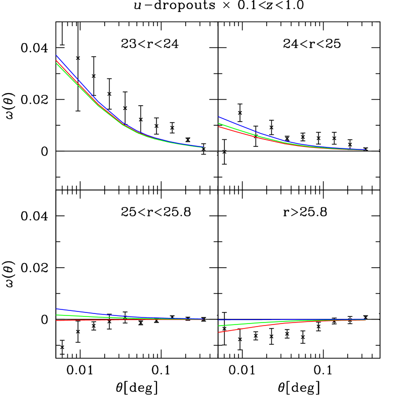
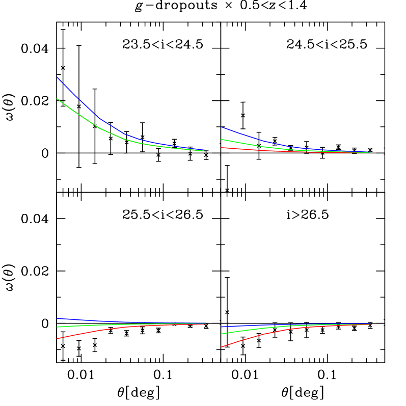
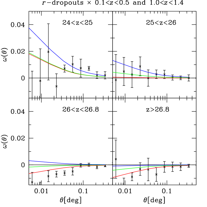
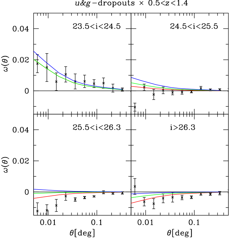
Figure 4: Cross-correlation functions between the dropouts at different redshifts and with different magnitudes and the different foreground galaxy samples. The red, green, and blue lines correspond to the predictions based on the LF slopes of Sawicki & Thompson (2006), Steidel et al. (1999), and Bouwens et al. (2007), respectively. For some background samples the predictions by Sawicki & Thompson (2006) and Steidel et al. (1999) are virtually identical so that the red and green curve lie on top of each other.

4.2 Interpretation of the observed signal

There is good qualitative agreement between the measured cross-correlation functions and the predictions from cosmic magnification. Bright LBGs show a strong positive cross-correlation to the foreground lenses, intermediately bright LBGs show a signal close to zero, and the faintest ones are anti-correlated. Especially the latter observation is a very strong argument for the lensing nature of the signal, since a physical cross-correlation caused by redshift overlap could not produce such an anti-correlation.

The magnification predictions are performed from Eq. 7 using the non-linear power spectrum in Peacock & Dodds (1996) with a biasing $b=1$. There is a general tendency of an underestimation of the signal by the theoretical predictions. This can have different reasons:

1. Lensing predictions are performed using the weak lensing approximation, i.e $(\kappa,\gamma)\ll 1$. Next order corrections are only of the order of 10% (Ménard et al., 2003).

2. The power spectrum normalisation $\sigma_{8}$ is probably also another minor contribution since it is unlikely that the real normalisation is very different from the fiducial $\sigma_{8}=0.8$.

3. The most likely explanation lies in the biasing parameter $b$ of the foreground galaxy population. Further investigation will be necessary, in particular the combined analysis with the foreground auto-correlation function could remove any direct dependence on $b$ (Van Waerbeke, 2009).

The predictions based on the LF measurements by Sawicki & Thompson (2006) seem to agree best with our data. The LFs by Bouwens et al. (2007) estimated from space-based data with their very steep faint-end slopes do not yield the negative amplitudes observed in our cross-correlation functions of the faintest LBGs. However, we cut the LBG samples in observed magnitudes while Bouwens et al. (2007) account for the asymmetric scatter at the faint end introduced by magnitude errors called Eddington bias (Eddington, 1913; Teerikorpi, 2004). The LBGs at the faint end of our samples have intrinsic magnitudes that are on average fainter than the observed ones due to this effect. Taking this into account would lead to more negative values for $\left<\alpha-1\right>$ and theoretical predictions with a larger negative amplitude. Interestingly, Sawicki & Thompson (2006) do not correct for that asymmetric scatter. We suspect that the better agreement of our data with the predictions based on their LFs originates from that fact.

The predictions based on the LF estimates from Steidel et al. (1999) lie in between the predictions from Sawicki & Thompson (2006) and Bouwens et al. (2007).

It has also been reported by Trenti & Stiavelli (2008) that cosmic variance can lead to a change in the shape of the LF, especially at the faint end. Pencil-beam surveys in under dense fields tend to yield steeper slopes than the cosmic average. That may well be another explanation for the discrepancy between our results and the predictions based on the HST measurements.

4.3 Optimally weighted cross-correlation functions

Next, we estimate optimally weighted cross-correlation functions as introduced by Ménard et al. (2003) and also used in Scranton et al. (2005). We weigh each galaxy with the $\alpha-1$ value corresponding to its magnitude and estimate the correlation function according to Eq. 12. This is done three times for the three different sets of LFs. The results for the LFs by Sawicki & Thompson (2006) are displayed in Fig. 5 together with the theoretical predictions. These are computed with Eq. 6 by taking the average squared weight, $\left<(\alpha-1)^{2}\right>$, as the pre-factor.

Figure 5: Optimally weighted cross-correlation function between the complete dropout samples and the different foreground galaxy samples. The solid line correspond to the predictions based on the LF slopes of Sawicki & Thompson (2006).

There is a similar tendency of the theoretical predictions being slightly lower than the observed signals, most serious for the $u$-dropouts. The same reasons as discussed in Sect. 4.2 apply here.

Table 2 summarises the results for the normal as well as the weighted correlation functions. For the optimally weighted cross-correlation functions we report the total significance of the detection as computed with the help of the covariance matrix. See Fig. 6 for an example of such a matrix.

Table 2: Basic quantities of the samples used in the cross-correlation analysis. The subscripts _ST, _St, and _Bo refer to the luminosity function estimates of Sawicki & Thompson (2006), Steidel et al. (1999), and Bouwens et al. (2007), respectively.

sample	No. of LBGs	$\left<\alpha-1\right>_{\rm ST}$	$\left<\alpha-1\right>_{\rm St}$	$\left<\alpha-1\right>_{\rm Bo}$	$\sigma_{\rm ST}$	$\sigma_{\rm St}\,^{a}$	$\sigma_{\rm Bo}\,^{a}$
$u$-dropouts
$23.0<r<24.0$	714	2.03	1.97	2.14
$24.0<r<25.0$	7263	0.55	0.62	0.77
$25.0<r<25.8$	15524	-0.02	0.10	0.24
$25.8<r$	10679	-0.29	-0.14	-0.01
$23.5<r$ (opt. weights)	34058	0.17	0.17b	0.24b	10.21	10.47	9.93
$g$-dropouts
$23.5<i<24.5$	990	1.28	1.28	1.78
$24.5<i<25.5$	7557	0.13	0.32	0.62
$25.5<i<26.5$	18948	-0.36	-0.08	0.12
$26.5<i$	8686	-0.56	-0.25	-0.08
$23.5<i$ (opt. weights)	36181	0.21b	0.10b	0.20b	6.95	7.08	5.46
$r$-dropouts
$24.0<z<25.0$	520	1.02	1.07	2.12
$25.0<z<26.0$	3482	0.04	0.25	0.74
$26.0<z<26.8$	4768	-0.37	-0.09	0.18
$26.8<z$	1685	-0.53	-0.23	-0.05
$23.5<z$ (opt. weights)	10471	0.20b	0.12b	0.51b	6.91	5.94	4.08
$u$&$g$-dropouts
$23.5<i<24.5$	5256	1.27	1.27	1.60
$24.5<i<25.5$	23212	0.18	0.33	0.54
$25.5<i<26.3$	26619	-0.26	-0.06	0.11
$26.3<i$	14358	-0.46	-0.23	-0.08
$23.5<i$ (opt. weights)	69445	0.24b	0.20b	0.33b	8.98	7.24	4.96

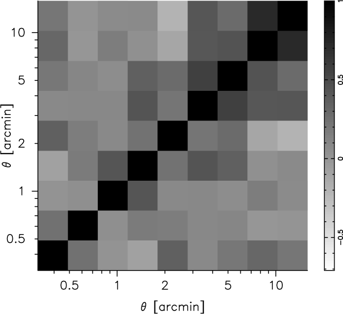
Figure 6: Correlation matrix (normalised covariance matrix) of the optimally-weighted cross-correlation function between $u$-dropouts and galaxies with $0.1<z_{\rm phot}<1.0$. We display the scales $0\aas@@fstack{\prime}3<\theta<15^{\prime}$ used for the estimation of the total significance.

4.4 Tests for systematics

In order to test for possible systematics we select stars from our catalogues via a cut in magnitude and half-light-radius and cross-correlate these to our LBG samples. The amplitudes of the normal cross-correlation functions are mostly consistent with zero in all magnitude bins and for all LBG redshifts. The optimally-weighted cross-correlation functions are all consistent with zero as well.

Furthermore, we checked the influence of the choice of the foreground sample. We included galaxies with photo-$z$ estimates in regions where we would expect some contamination of the LBG samples. For example, including galaxies with $z_{\rm phot}<0.5$ into the foreground sample that is cross-correlated to the $g$-dropouts leads to a boost in the amplitudes. In particular, the anti-correlations, which were observed before when excluding this low-$z$ range, vanish. The signal turns positive for the faintest $g$-dropouts. This is in clear contradiction to the predicted lensing signal which should be negative because of the shallow slope of the LF at the faint end. Similarly, the negative signal for the faintest $r$-dropouts turns positive if galaxies with $0.5<z_{\rm phot}<1.0$ are included in the foreground sample. These excess signals can be explained by redshift overlap leading to physical cross-correlations between the small number of contaminants of the LBG samples and the foreground galaxies.

But then, the fact that we do see negative cross-correlations of the expected amplitude and angular dependence when these problematic foreground redshifts are excluded from the low-$z$ sample is a strong argument for the robustness of the analysis. While a small fraction of low-$z$ contaminants is probably still present in our background LBG samples these do not change the amplitude or the shape of the signal but only add noise since they do not carry a lensing signal.

5 Conclusions

For the first time we detect cosmic magnification in samples of normal galaxies. With the help of the Lyman-break technique we select background samples of high surface density and large lensing efficiency (due to their high redshifts) from data of the CFHTLS-Deep survey. We cross-correlate these LBGs to low-$z$ foreground galaxies which we select by accurate photo-$z$’s. The expected signals are estimated by taking external LBG-LF estimates from the literature. There is good agreement between the observed signals and the theoretically predicted ones in amplitude as well as in angular dependence. Some deviations can be explained by Eddington bias, the linearisation of the magnification, and uncertainties in the cosmological parameters. The LBG samples used here represent the highest redshift population that has been used in weak gravitational lensing so far.

Having proven that cosmic magnification with normal galaxies works in practice we plan to apply this technique to large imaging surveys in the future. In contrast to cosmic magnification measurements with QSOs, using galaxies as sources has the advantage of much higher source densities. Also compared to cosmic shear and galaxy-galaxy-lensing this technique might prove competitive since the number of source galaxies with accurate magnitude measurements and photo-$z$’s (the only requirements for magnification measurements) considerably exceeds the number of sources with accurate shape measurements. Although magnification measurements are less powerful than shear measurements for a given sample of galaxies, the larger densities that can be reached with future ground-based surveys will make precision measurements of cosmic magnification very attractive. A precise calibration of the LFs of the source galaxies and a robust correction for observational bias like the Eddington bias is, however, mandatory to reach that goal.

The cosmological constraints derived from cosmic magnification measurements will be complementary to other probes such as cosmic shear because their dependence on redshift is slightly different. This can potentially lead to breaking degeneracies in cosmological parameters. See also the theoretical companion paper by Van Waerbeke (2009) about this topic. Furthermore, cosmic magnification depends on completely different systematics. Measuring the same cosmological quantity with e.g. cosmic shear and cosmic magnification simultaneously will be an extremely important consistency check. Thus, cosmic magnification and cosmic shear can become a powerful combination in unravelling the mysteries of dark matter and dark energy.