Entanglement entropy in quantum impurity systems and systems with boundaries

Abstract

We review research on a number of situations where a quantum impurity or a physical boundary has an interesting effect on entanglement entropy. Our focus is mainly on impurity entanglement as it occurs in one dimensional systems with a single impurity or a boundary, in particular quantum spin models, but generalizations to higher dimensions are also reviewed. Recent advances in the understanding of impurity entanglement as it occurs in the spin-boson and Kondo impurity models are discussed along with the influence of boundaries. Particular attention is paid to $1+1$ dimensional models where analytical results can be obtained for the case of conformally invariant boundary conditions and a connection to topological entanglement entropy is made. New results for the entanglement in systems with mixed boundary conditions are presented. Analytical results for the entanglement entropy obtained from Fermi liquid theory are also discussed as well as several different recent definitions of the impurity contribution to the entanglement entropy.

1 Introduction

The definition of entanglement entropy is based on dividing space into two regions. In many cases the systems under study are homogenuous and this division is purely fictitious. However, there has also been considerable activity on studying entangelement in inhomogeneous systems, the simplest of which contain physical boundaries or a single impurity. There are currently several useful measures of entanglement, here we shall use the von Neumann entanglement entropy as defined by dividing a bipartite system in a pure state at $T=0$ into 2 regions, $A$ and $B$. From the ground state pure density matrix, region $B$ is traced over to define the reduced density matrix $\rho_{A}$. In most cases we shall take $A$ to include the impurity/boundary. From this the von Neumann entanglement entropy [1, 2],

$$S(r,R)\equiv-\Tr[\rho_{A}\ln\rho_{A}]$$ (1.1)

is obtained for a subsystem of size $r$ inside a larger system of size $R$. There are several motivations for this work.

One motivation is to study models of a qubit interacting with a decohering enviroment [3, 4, 5, 6]. Such a system is often represented by a 2-level system, or spin-1/2, interacting with an otherwise homogeneous, and often one-dimensional medium with gapless excitations. Some versions of this model are equivalent to the Kondo model, motivating studies of ground state entanglement of an impurity spin with the conduction electrons in Kondo models. This entanglement entropy can be easily expressed exactly in terms of the impurity magnetization, which, for many models, has been well-understood many years ago [5, 7]. This single site impurity entanglement, which we denote by $s_{\mathrm{imp}}$, is reviewed in section 2.

Another motivation comes from the thermodynamic impurity entropy, $\ln g$, which was calculated by Bethe ansatz [8, 9] for multi-channel Kondo models and then discussed more generally from the viewpoint of Conformal Field Theory (CFT) [10]. General quantum impurity models, such as occur in condensed matter physics, were argued to renormalize to conformally invariant boundary conditions, and $\ln g$ was argued to be a universal quantity depending only on the boundary condition. Calabrese and Cardy (C & C) [11] argued that, for a CFT defined on the semi-infinite line with a conformally invariant boundary condition (CIBC) at the end, the entanglement of a region of length $r$ with the rest is given by [12, 13, 14, 11]:

$$S(r)=\frac{c}{6}\ln\left(\frac{r}{a}\right)+\ln g+s_{1}/2.$$ (1.2)

$\ln g$ depends on the CIBC, establishing a surprising connection between thermodynamic and entanglement entropy. Here $a$ is a cut-off length scale and $s_{1}$ is a non-universal number. Both are independent of the CIBC. In the numerical work one-dimensional tight binding models are generally considered in which case $a$ is the lattice constant. This raised the possibility that this impurity part of the entanglement entropy, $S_{\mathrm{imp}}$, might exhibit universal renormalization group (RG) behavior and this was confirmed in studies of spin chains with a boundary magnetic field [15] and of the Kondo model [16, 7]. The connection between the thermodynamic impurity entropy and the impurity entanglement entropy is outlined in section 3.

There is a deep connection between (1+1) dimensional CFT and topological phases of gapped (2+1) dimensional systems such as occur in the fractional quantum Hall effect. While the entanglement entropy of a region in a gapped 2 dimensional (2D) system is expected to grow with the length of its perimeter, it was shown that there is an additional universal, length independent “ topological entropy” [17, 18], $-\ln{\cal D}$ which can be extracted from the corresponding (1+1) dimensional CFT. The connection between the boundary entropy of C & C [11] and the topological entropy can be clarified by considering a (2+1) dimensional system with boundaries, a “Hall bar”, containing a point contact. There are gapless degrees of freedom living on the edge of the Hall bar described by a CFT. (See Fig. 9.) The point contact may renormalize to a CIBC, corresponding to breaking the Hall bar into two pieces and the change in topological entropy due to this renormalization can be related to the change in the boundary entropy, $\ln g$. As we will show, this is defined in terms of the entanglement of a section of the Hall bar of length $r$, containing the point contact with the rest of the (infinite) Hall bar. The connection with topological phases is discussed in section 3.3.

An alternative type of impurity-related entanglement entropy has also been studied for a 1D wire with a point defect, which if relevant, effective breaks the system in two at low energies [19, 20, 21]. Rather than studying the entanglement of a finite region surrounding the point contact and extracting the $\ln g$ term in Eq. (1.2) instead the entanglement of one side of the point contact with the other was studied. In cases where the point defect is relevant, it was found that this entanglement tends to vanish with increasing system size, again verifying that entanglement entropy exhibits RG flow behavior. This type of impurity entanglement is discussed in section 4.

A surprising result of numerical studies of entanglement entropy in 1D antiferromagnets with boundaries was the presence of an alternating term decaying away from the boundaries [22, 7]. Although a theory of this is still lacking, it was shown numerically to track closely the energy density as a function of distance from the boundary and a heuristic understanding was obtained in terms of a local dimerization induced by the boundary, related to “resonating valence bonds”. This boundary induced alternation in the entanglement entropy is reviewd in section 5.

Although probably less useful as a model of a decohering environment and not related to CFT and universal RG concepts, impurity entanglement entropy has also been studied for gapped (1+1) dimensional systems, including dimerized and Haldane gap spin chains. This aspect is reviewed in section 6.

As a final motivation, we note that recent models for qubit teleportation and quantum state transfer using quantum spin chains [23, 24, 25, 26, 27, 28, 29, 30, 31] employ models closely related to the quantum spin models reviewed and in many cases rely on properties of the entanglement arising from the impurities reviewed here.

2 The single site impurity entanglement entropy, $s_{\mathrm{imp}}$

The simplest definition of the impurity entanglement is to consider the (single site) impurity as sub-system $A$ and the rest of the system as sub-system $B$. A measure of the impurity entanglement is then simply given by the von Neumann entanglement entropy of the reduced density matrix for $A$ inside a system of total size $R$. Since $A$ describes just a single site one often refers to this as the single site impurity entanglement. We shall denote this quantity by $s_{\mathrm{imp}}$ to distinguish it from $S_{\mathrm{imp}}(r,R)$ defined in later sections by the difference in the uniform part of the von Neumann entanglement entropy for a sub-system of extent $r$ with and without the impurity present. Since $s_{\mathrm{imp}}$ is concerned with a single site such a definition through a subtraction is not possible and the explicit $r$ dependence through the size of the sub-system $A$ is absent.

The single site impurity entanglement, $s_{\mathrm{imp}}$, has been studied mainly in 2 different settings: The spin-boson model [32, 4, 5, 6] and the closely related Kondo model [7]. For the case where the impurity is a $s=1/2$ system (qubit) it is easy to see [32, 4, 7] that:

$$s_{\mathrm{imp}}=-\sum_{\pm}(1/2\pm m_{\mathrm{imp}})\ln[(1/2\pm m_{\mathrm{imp}})],$$ (2.1)

$m_{\mathrm{imp}}$ being the magnetization of the impurity in the ground-state. For a system with a singlet ground state $m_{\mathrm{imp}}=0$ and $s_{\mathrm{imp}}$ is maximal [3], the qubit is maximally entangled with the rest of the system. For a system with a doublet ground-state ($R$ odd) the behavior of $m_{\mathrm{imp}}$ is more interesting and exhibits the usual cross over associated with Kondo physics. In this case $m_{imp}$ was studied, for the usual fermion Kondo model, in [33] and [34, 35] for example from which $s_{\mathrm{imp}}$ can be derived.

The spin-boson model is defined by:

$$H_{SB}=-\frac{\Delta}{2}\sigma_{x}+\frac{h}{2}\sigma_{z}+H_{osc}+\frac{1}{2}\sigma_{z}\sum_{q}\lambda_{q}(a_{q}+a_{q}^{\dagger}),$$ (2.2)

where $\sigma_{x}$ and $\sigma_{z}$ are Pauli matrices and $\Delta$ is the tunneling amplitude between the states with $\sigma_{z}=\pm 1$. $H_{osc}$ is the Hamiltonian of an infinite number of harmonic oscillators with frequencies $\{\omega_{q}\}$, which couple to the spin degree via $\{\lambda_{q}\}$. The heat bath is characterized by its spectral function $J(\omega)\equiv\pi\sum_{q}\lambda_{q}^{2}\delta(\omega_{q}-\omega)=2\pi\alpha\omega,\ \omega\ll\omega_{c}$ (Ohmic heat bath). Efficient NRG calculations can be performed on this model through a mapping [36] to the anisotropic Kondo model. This allowed for rather detailed NRG studies [32] of $s_{\mathrm{imp}}$ as a function of $\alpha$. Exploiting known exact results for $\langle\sigma_{z}\rangle$ and $\langle\sigma_{x}\rangle$ in the spin-boson problem it has been shown [4] that $s_{\mathrm{imp}}$ in several limits is a universal function of $h/T_{K}$, where $T_{K}$ is the Kondo scale. For $T_{K}\ll h\ll\Delta$ it was found [4] that:

$$\lim_{T_{K}\ll h\ll\Delta}s_{\mathrm{imp}}(\alpha,\Delta,h)=k_{2}(\alpha)\left(\frac{T_{K}}{h}\right)^{2-2\alpha}\ln\left(\frac{h}{T_{K}}\right),$$ (2.3)

with $k_{2}(\alpha)$ a known cut-off independent funtion so that $s_{\mathrm{imp}}$ in this limit is a universal function of $h/T_{K}$. On the other hand, for $h\ll T_{K}\ll\Delta$ it can be shown that:

$$\lim_{h\ll T_{K}\ll\Delta}s_{\mathrm{imp}}(\alpha,\Delta,h)=s_{\mathrm{imp}}(\alpha,\Delta,0)-k_{1}(\alpha)\left(\frac{h}{T_{K}}\right)^{2},$$ (2.4)

with $k_{1}(\alpha)$ a known cut-off independent function. However, in this case $s_{\mathrm{imp}}(\alpha,\Delta,0)$ is in general non-universal and only the second term exhibits scaling.

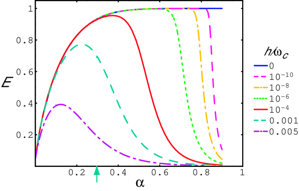
Figure 1: $s_{\mathrm{imp}}(\alpha,\Delta=0.01\omega_{c},h)$ ($E$ on the figure label) as a function of $\alpha$ for a range of $h/\omega_{c}$. Reproduced with permission from [4].

The general results are illustrated in Fig. 1 where $s_{\mathrm{imp}}(\alpha,\Delta=0.01\omega_{c},h)$ ($E$ on the figure label) is plotted versus $\alpha$ for a range of $h/\omega_{c}$. For $h=0$ $s_{\mathrm{imp}}(\alpha)$ is a monotonically increasing function where as for non-zero $h$ a maximum associated with the crossover $h\sim T_{K}$ occurs. The case of a sub-Ohmic heat bath has also been studied [5].

The usual Kondo Hamiltonian [37, 38] contains a Heisenberg interaction between a $s=1/2$ impurity spin, $S$, and otherwise non-interacting electrons. A simple model takes a free electron dispersion relation and a $\delta$ -function Kondo interaction:

$$H=\int d^{3}r[\psi^{\dagger}(-\nabla^{2}/2m)\psi+J_{K}\delta^{3}(\vec{r})\psi^{\dagger}(\vec{\sigma}/2)\psi\cdot\vec{S}].$$ (2.5)

(Actually, an ultra-violet cut-off of the $\delta$-function interaction is necessary for the model to be completely well-defined.) In the ground-state of the Kondo model the impurity spin is screened by the conduction electrons through the formation of a singlet. This phenomenon is expected to take place on a length scale:

$$\xi_{K}=v/T_{K}\propto e^{1/(\nu J_{K})},$$ (2.6)

where $\nu$ is the density of states per spin band , $T_{K}$ is the Kondo scale and $v$ the velocity of the fermions. Due to the $\delta-$ function form of the interaction Eq. (2.5) can be reduced to a one-dimensional model which can be represented by a lattice model of finite extent $R$ (including the impurity), suitable for numerical studies. As outlined above and discussed in more detail in section 3.2, we expect the case of $R$ odd to reflect Kondo physics and possibly scaling with $R/\xi_{K}$. However, it has been shown [7] that $s_{\mathrm{imp}}$ exhibits weak scaling violations from the expected $R/\xi_{K}$ scaling. In particular, $m_{\mathrm{imp}}$ was shown to take the form:

$$m_{\mathrm{imp}}\sim\frac{1}{2}-\left[\frac{J_{K}}{\pi v}\right]^{2}\ln(R/a),$$ (2.7)

where $a$ is a short distance cut off. Hence weak scaling violations are present in $m_{\mathrm{imp}}$ and therefore also in $s_{\mathrm{imp}}$ even though $s_{\mathrm{imp}}$ clearly displays the expected crossover related to Kondo physics.

Figure 2: (a) Weak scaling violations for the single site impurity entanglement entropy $s_{imp}$ (a) [Eq. (2.1)] and the local impurity magnetization $m_{imp}=\langle S_{1}^{z}\rangle$ (b). All data are for odd length chains between $R=19\ldots 101$. Reprinted from [7].

The presence of such scaling violations is illustrated in Fig. 2.

Finally, recent work has focused on the entanglement between the 2 impurity spins in the two-impurity Kondo model [39, 3, 40] as well as the pair-wise entanglement between end spins in open ended Heisenberg spin chains [41].

3 Impurity entropies from the CFT perspective

In this section we review the concept of thermodynamic impurity entropy and its connection with CFT. We also connect it with topological entropy in 2D topological insulators and discuss various applications of these general ideas to specific models: spin chains with boundary fields, Kondo model and point contact in a Hall bar.

3.1 Thermodynamic Impurity Entropy

Thermodynamic impurity entropy can be measured experimentally from impurity specific heat using the thermodynamic identity:

$$C=T{\partial S\over\partial T}.$$ (3.1)

The impurity contribution to the specific heat, and hence the entropy, can be measured by subtracting off the same quantity for the pure system. Such measurements and related theoretical calculations have been performed for many years in Kondo impurity systems.

$C(T)$ for a metal with a dilute random array of magnetic impurities is measured and $C(T)$ for the pure system is subtracted off. Dividing by the number of impurities and extrapolating to zero impurity density gives the contribution to the specific heat of a single impurity, $C_{\mathrm{imp}}(T)$. From integrating $C_{\mathrm{imp}}(T)/T$ one can, at least in principle, obtain $S^{\mathrm{Th}}_{\mathrm{imp}}(T)$. We consider the infinite volume limit, so that $S^{\mathrm{Th}}_{\mathrm{imp}}(T)$ becomes a function of $T$ only. We may formally define $S^{\mathrm{Th}}_{\mathrm{imp}}(T)$ by calculations on a 1D system of length $R$ with a single impurity:

$$S^{\mathrm{Th}}_{\mathrm{imp}}(T)\equiv\lim_{R\to\infty}[S(T,R)-S_{0}(T,R)].$$ (3.2)

Here $S(T,R)$ is the thermodynamic entropy with the impurity present and $S_{0}(T,R)$ is the same quantity without the impurity. $S^{\mathrm{Th}}_{\mathrm{imp}}(T)$ exhibits interesting $T$-dependence which reflects the RG flow of the Kondo model. It can be calculated with high precision from the Bethe ansatz solution of the Kondo model first derived by Andrei [42] and Wiegmann [43]. In the limit of a weak bare Kondo coupling $S^{\mathrm{Th}}_{\mathrm{imp}}(T)\approx\ln 2$ at $T\gg T_{K}$ and $S^{\mathrm{Th}}_{\mathrm{imp}}(T)\to 0$ at $T\ll T_{K}$. This reflects the fact that the bare coupling of the magnetic impurity to the conduction electrons is very weak so that we obtain essentially the full entropy of a free spin-1/2, $\ln 2$ at $T\gg T_{K}$. However, as the temperature is lowered the spin is “screened” i.e. it goes into a singlet state and the impurity entropy is accordingly lost. The asymptotic values of $S^{\mathrm{Th}}_{\mathrm{imp}}(T)$ at high and low temperatures are characteristic of the RG fixed points of the Kondo Hamiltonian.

The $k$-channel Kondo model

$$H=\int d^{3}r\sum_{i=1}^{k}[\psi^{\dagger i}(-\nabla^{2}/2m)\psi_{i}+J_{K}\delta^{3}(\vec{r})\psi^{\dagger i}(\vec{\sigma}/2)\psi_{i}\cdot\vec{S}].$$ (3.3)

also has $S^{\mathrm{Th}}_{\mathrm{imp}}(T)\approx\ln 2$ at $T\gg T_{K}$. However, it was found, from the Bethe ansatz solution, that at $T\to 0$ it has the limiting value $\ln g$ where [10]:

$$g=2\cos[\pi/(2+k)]\leq 2.$$ (3.4)

Heuristically, $g$ represents a “fractional ground state degeneracy” characterizing the non-Fermi liquid ground state of the overscreened Kondo model.

The interesting behavior of the impurity entropy in the multi-channel Kondo model was later shown to be a special case of a general phenomenon in quantum impurity models. Many models of this type have low energy descriptions in terms of 1D CFT’s. Quite general boundary conditions and boundary interactions are expected to renormalize, at low energies, to CIBC’s. Cardy showed that generally CIBC’s can be associated with boundary states, $|A>$. The conformally invariant partition function defined on a strip of length $R$, at inverse temperature $\beta$, with CIBC’s $A$ and $B$ at the two ends can be written:

$$Z_{AB}=\mathrm{tr}e^{-\beta H^{R}_{AB}},$$ (3.5)

where $H^{R}_{AB}$ is the Hamiltonian on an interval of length $R$ with BC’s $A$ and $B$ at the two ends. Alternatively, we may switch space and imaginary time directions and write:

$$Z_{AB}=<A|e^{-RH^{\beta}_{P}}|B>.$$ (3.6)

Now the system propagates for time $R$, under the action of the Hamiltonian defined on a periodic interval of length $\beta$ with initial and final states $|A>$ and $|B>$. The boundary states can be expanded in a complete basis of Ishibashi states, associated with each conformal tower, $a$:

$$|A>=\sum_{a}|a><a0|A>.$$ (3.7)

(The Ishibashi states $|a>$ are sums over all descendants with equal weight in left and right-moving sectors.) Thus, we may write:

$$Z_{AB} = \sum_{a}<A|a0><a0|B><a|e^{-RH^{\beta}_{P}}|a>$$ (3.8)

$$= \sum_{a}<A|a0><a0|B>\chi_{a}(e^{-4\pi R/\beta})$$

where $\chi_{a}$ is the character of the $a^{\mathrm{th}}$ conformal tower. Written in this form it is straightforward to extract the impurity entropy. Taking the limit $R\gg\beta$ only the highest weight state in the conformal tower of the identity operator contributes, giving:

$$Z_{AB}\to e^{\pi Rc/6\beta}<A|00><00|B>.$$ (3.9)

(Here $c$ is the central charge associated with the bulk CFT.) From this expression we obtain the entropy:

$$S^{\mathrm{Th}}_{AB}={\partial\over\partial T}[T\ln Z_{AB}]={\pi RcT\over 3}+\ln g_{AB}$$ (3.10)

where:

$$g_{AB}=g_{A}\cdot g_{B}=<A|00><00|B>.$$ (3.11)

This consists of the bulk term, independent of the boundary conditions and proportional to the system size, $R$, as well as the boundary term $\ln g$ which is a sum of contributions from each boundary. Using the known boundary state corresponding to the non-Fermi liquid ground state of the multi-channel Kondo model we can reobtain the Bethe ansatz result for $S^{\mathrm{Th}}_{\mathrm{imp}}(T=0)$ from this general CFT formula.

$\ln g$, the $T=0$ thermodymamic entropy, is a universal property of fixed points of the boundary RG. It has the interesting property that it always decreases under RG flow from an unstable to stable fixed point [10]. Eq. (3.4) provides an example of this: the impurity entropy is $\ln 2$ at the unstable fixed point, $T\gg T_{K}$, and always has a smaller value at the stable fixed point which occurs at $T=0$.

3.2 Boundary term in the entanglement entropy

We now consider a semi-infinite CFT ($r\geq 0$) with CIBC, of type $A$ at $r=0$. We consider the ground state entanglement entropy for the region, $0\leq r^{\prime}\leq r$, $S_{A}(r)$. We might now expect some additional term in $S(r)$, $c_{A}$, which depends on the CIBC $A$, but not on the length of the region under consideration, $r$:

$$S_{A}(r)=\frac{c}{6}\ln\left(\frac{r}{a}\right)+c_{A}+\frac{s_{1}}{2}.$$ (3.12)

We can argue that $c_{A}=\ln g_{A}$, the thermodynamic impurity entropy, by the device of considering the entanglement entropy for this system at finite temperature. C&C [11] showed that the generalization of $S_{A}(r)$ to a finite inverse temperature, $\beta$, is given by a standard conformal transformation:

$$S_{A}(r,\beta)=\frac{c}{6}\ln\left[\frac{\beta}{\pi a}\sinh\left(\frac{2\pi r}{\beta}\right)\right]+c_{A}+s_{1}/2.$$ (3.13)

See also [14]. $S_{A}(r,\beta)$ is defined by beginning with the Gibbs density matrix for the entire system, $e^{-\beta H}$ and then again tracing out the region $r^{\prime}>r$. Now consider the high temperature, long length limit, $\beta\ll r$:

$$S_{A}\to\frac{2\pi cr}{6\beta}+\frac{c}{6}\ln\left(\frac{\beta}{2\pi a}\right)+c_{A}+\frac{s_{1}}{2}+O(e^{-4\pi r/\beta}).$$ (3.14)

The first term is the extensive term (proportional to $r$) in the thermodynamic entropy for the region, $0<r^{\prime}<r$. The reason that we recover the thermodynamic entropy when $r\gg\beta$ is because, in this limit, we may regard the region $r^{\prime}>r$ as an “additional reservoir” for the region $0\leq r^{\prime}\leq r$. That is, the thermal density matrix can be defined by integrating out degrees of freedom in a thermal reservoir, which is weakly coupled to the entire system. On the other hand, the region $r^{\prime}>r$ is quite strongly coupled to the region $r^{\prime}<r$. Although this coupling is quite strong, it only occurs at one point, $r$. When $r\gg\beta$, this coupling only weakly perturbs the density matrix for the region $r^{\prime}<r$. Only low energy states, with energies of order $1/r$ and a neglegible fraction of the higher energy states (those localized near $r^{\prime}=r$) are affected by the coupling to the region $r^{\prime}>r$. The thermal entropy for the system, with the boundary at $r=0$ in the limit $r\gg\beta$ is:

$$S^{\mathrm{Th}}_{A}\to\frac{2\pi cr}{6\beta}+\ln g_{A}+\mathrm{constant},$$ (3.15)

with corrections that are exponentially small in $r/\beta$. The only dependence on the CIBC, in this limit, is through the constant term, $\ln g_{A}$, the impurity entropy. Thus it is natural to identify the BC dependent term in the entanglement entropy with the BC dependent term in the thermodynamic entropy:

$$c_{A}=\ln g_{A}.$$ (3.16)

This follows since, in the limit, $r\gg\beta$, we don’t expect the coupling to the region $r^{\prime}>r$ to affect the entanglement entropy associated with the boundary $r^{\prime}=0$, $c_{A}$. Note that the entanglement entropy, Eq. (3.14), contains an additional large term not present in the thermal entropy. We may ascribe this term to a residual effect of the strong coupling to the region $r^{\prime}>r$ on the reduced density matrix. However, this extra term does not depend on the CIBC as we would expect in the limit $r\gg\beta$ in which the “additional reservoir” is far from the boundary. Now passing to the opposite limit $\beta\to\infty$, we obtain the remarkable result that the only term in the (zero temperature) entanglement entropy depending on the BC is precisely the impurity entropy, $\ln g_{A}$, Eq. (1.2). We may also consider a finite system, of length $R$, with ICBC at both ends. In the case, where both BC’s are the same, $A$, we expect the generalization of Eq. (1.2) which follows from a conformal transformation:

$$S_{A}(r,R)=\frac{c}{6}\ln\left[\frac{2R}{\pi a}\sin\left(\frac{\pi r}{R}\right)\right]+\ln g_{A}+\frac{s_{1}}{2},$$ (3.17)

with the equivalent result for periodic boundary conditions:

$$S^{\mathrm{PBC}}_{A}(r,R)=\frac{c}{3}\ln\left[\frac{R}{\pi a}\sin\left(\frac{\pi r}{R}\right)\right]+s_{1}.$$ (3.18)

As usual, $a$ denotes the lattice spacing. A result has not been obtained, as far as we know, for the case where the CIBC’s are different at the two ends.

As discussed in the previous sub-section, the thermodynamic impurity entropy, $\ln g$, is a universal quantity with interesting RG behavior. It is then natural to expect that the impurity term in the entanglement entropy will behave similarly. In particular, consider beginning with a CFT on the semi-infinite line with CIBC $A$ and then adding a small relevant boundary interaction:

$$H=H_{\mathrm{CFT}}-\lambda\phi(0)$$ (3.19)

where $\phi$ has an RG scaling dimension $y<1$. ($y=1$ is the marginal dimension for boundary interactions, since the action contains only a time-integral over $\phi(\tau,r=0)$ and no spatial integral.) We expect that, under the renormalization group, the Hamiltonian will flow to an infrared stable fixed point, at long length scales, characterized by some other CIBC, $B$. The “g-theorem” [10, 44] implies that the thermodynamic impurity entropy at the stable fixed point obeys $g_{B}<g_{A}$. Typically the flow between fixed points can be controlled by introducing a finite length scale which acts as an infrared cut off. This is often done by putting the system in a finite box, of size $R$. It is not obvious what will happen when we have no physical box but introduce a length scale $l$ by the definition of the entanglement entropy. Will the impurity part of the entanglement entropy exhibit a cross over from $g_{A}$ to $g_{B}$ as we increase $l$? Will this cross over be universal? These questions have been investigated numerically, using the DMRG method, in a couple of models.

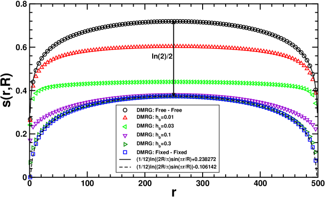
Figure 3: $S(r,R)$ versus $r$ ($R=500$) for the transverse field Ising model calculated using DMRG with $m=128$. Results are shown for free-free and fixed-fixed boundary conditions along with four different values of $h_{b}=0.01,0.03,0.10,0.30$. For the numerical DMRG data only every 4th point is shown for clarity. The solid and dashed lines represent fits of the DMRG results for free-free and fixed-fixed BC’s, respectively, to the analytical result Eq. (3.17). For the latter case calculations were performed formally with $h_{b}=\infty$.

The first model considered was the 1D transverse field Ising model with a longitudinal boundary magnetic field [15]:

$$H=-\sum_{j=0}^{\infty}(S^{z}_{j}S^{z}_{j+1}+(1/2)S^{x}_{j})+h_{b}S^{z}_{0}.$$ (3.20)

The bulk transverse field has been tuned to its critical value, $1/2$. A weak longitudinal field, $h_{b}$ is applied at the boundary, $j=0$, only. This boundary field is relevant, with dimension 1/2 and therefore induces a boundary RG flow between the only two boundary fixed points in this model, corresponding to free or fixed BC. The values of $g$ are $g=1$ (free) and $g=1/\sqrt{2}$ (fixed). DMRG results on chains of length up to 800, keeping 140 block states, showed quite convincingly that the entanglement entropy crosses over from $(1/12)\ln(r/a)$ to $(1/12)\ln(r/a)-(1/2)\ln 2$ as $r$ is increased from small values to values larger than a cross-over scale, $\xi$, determined by $h_{b}$ as $\xi\propto|h_{b}|^{-1/2}$. In figure 3 we illustrate these results by calculations on systems with $R=500$. In figure 4 we also show the entanglement entropy with different BC’s at the ends of a finite chain, fixed-free and fixed up-fixed down. As far as we know, no analytic formulas have been derived for these cases. We note that the expression:

$$S(r,R)={1\over 12}\ln\left[{R\over a}\sin\left({\pi r\over R}\right)\right]-\ln\left[\cos\left({\pi r\over 4R}\right)\right]+\hbox{constant}$$ (3.21)

seems to fit the data quite well in the fixed-free case.

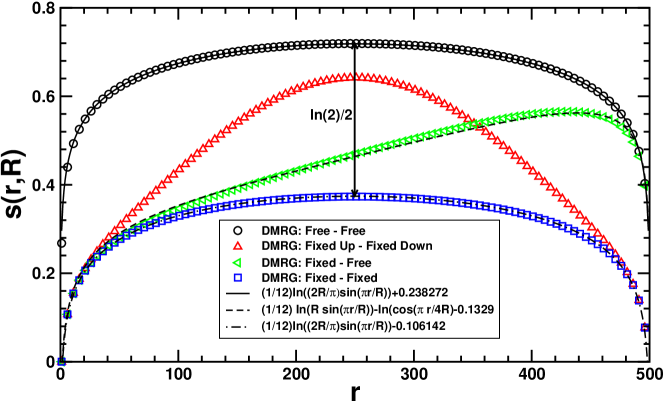
Figure 4: $S(r,R)$ versus $r$ ($R=500$) for the transverse field Ising model calculated using DMRG with $m=128$. Results are shown for free-free and fixed-fixed boundary conditions along with free-fixed and fixed (up) - fixed (down) boundary conditions. For the numerical DMRG data only every 4th point is shown for clarity. The solid and dashed lines represents fits of the DMRG data for free-free and fixed-fixed BC’s, respectively, to the analytical result Eq. (3.17). The calculations with fixed boundaries are performed by formally setting $h_{b}=\pm\infty$.

The second model in which this crossover was studied is the Kondo model [16, 7] For this model, we may consider the entanglement of a region inside a sphere of size $r$ surrounding the impurity, with the rest of space which may either be infinite or confined to a larger sphere of size $R$. The impurity entanglement entropy is defined as the increase in entanglement arising when the impurity is added to the system. This mimics the definition of the impurity thermodynamic entropy which has been well-studied experimentally and theoretically for Kondo systems. Due the $\delta$-function form of the Kondo-interaction, the 3D model is equivalent to a 1D model. To see this, we expand the electron fields in spherical harmonics. Only the s-wave interacts with the impurity spin, the other harmonics being completely free. The entanglement entropy may be written as a sum of contributions from each spherical harmonic:

$$S=\sum_{l,m}S_{l,m}.$$ (3.22)

Only the s-wave part, $S_{0,0}$ is affected by the Kondo interaction so that the total impurity entanglement entropy is given by the change in $S_{0,0}$ when the impurity spin is added. Assuming that the Kondo coupling is weak, as is usually the case in experiments, we may integrate out Fourier components of the s-wave electron fields except for a narrow band around the Fermi sphere. Linearizing the dispersion relation near the Fermi energy:

$$k^{2}/2m\approx k_{F}^{2}/2m+v_{F}(k-k_{F}),$$ (3.23)

the model becomes equivalent to a relativistic Dirac fermion defined on the half-line, $r>0$ interacting with the impurity spin at $r=0$:

$$H_{1D}\approx (iv_{F}/2\pi)\int_{0}^{R}dr[\psi_{L}^{\dagger}(d/dr)\psi_{L}-\psi_{R}^{\dagger}(d/dr)\psi_{R}]$$ (3.24)

$$+v_{F}\lambda_{K}\psi_{L}^{\dagger}(0)(\vec{\sigma}/2)\psi_{L}(0)\cdot\vec{S}.$$

Here $\lambda_{K}\propto J$ and a boundary condition:

$$\psi_{L}(0)=-\psi_{R}(0)$$ (3.25)

is imposed on the left and right movers.

To obtain a model amenable to DMRG studies, we could consider a 1D tight-binding version of this 1D continuum model. However, considerable numerical speed-up can be obtained by considering a “spin-only” version of the model. This is based on spin-charge separation for 1D interacting fermion systems, which follows from bosonization. We find that only the spin degrees of freedom of the 1D electrons interact with the impurity, when it is at the end of the chain. [Things are more complicated when it is not at the end. The simplifications at the end arise from the BC of Eq. (3.25).] The spin part of the Hamiltonian, the only part involving the Kondo interaction, can be written as a perturbed $SU(2)_{1}$ Wess-Zumino-Witten non-linear $\sigma$-model with Hamiltonian:

$$H_{s}=(v_{F}/2\pi)\int_{0}^{R}dr(1/3)[\vec{J}_{L}\cdot\vec{J}_{L}+\vec{J}_{R}\cdot\vec{J}_{R}]+v_{F}\lambda_{K}\vec{J}_{L}(0)\cdot\vec{S}.$$ (3.26)

Here $\vec{J}_{L/R}(r)$ are the spin density operators for left and right movers, with the BC

$$\vec{J}_{L}(0)=\vec{J}_{R}(0).$$ (3.27)

This implies that we may regard $\vec{J}_{R}(r)$ as the analytic continuation of $J_{L}(r)$ to the negative $r$ axis:

$$J_{R}(r)=\vec{J}_{L}(-r)$$ (3.28)

and write the theory in terms of left movers only defined on the interval $-R<r<R$:

$$H_{s}=(v/6\pi)\int_{-R}^{R}dr\vec{J}_{L}\cdot\vec{J}_{L}+v_{F}\lambda_{K}\vec{J}_{L}(0)\cdot\vec{S}.$$ (3.29)

Now consider Heisenberg antiferromagnetic S=1/2 chain with one weak link at the end:

$$H=J_{K}^{\prime}\vec{S}_{1}\cdot\vec{S}_{2}+\sum_{r=2}^{R-1}\vec{S}_{r}\cdot\vec{S}_{r+1}.$$ (3.30)

For $J_{K}^{\prime}\ll 1$ essentially the same low energy continuum limit field theory, Eq. (3.26) is obtained except that the Fermi velocity, $v_{F}$ is replaced by the spin-velocity, which we call $v$. This model is considerably more efficient to study with DMRG since there are only 2 states per site rather than 4. Actually, a drawback of this model is that there is an important marginally irrelevant bulk interaction in the low energy Hamiltonian:

$$\delta H=-(gv/2\pi)\vec{J}_{L}\cdot\vec{J}_{R}.$$ (3.31)

with the positive dimensionless coupling constant $g$ of O(1). This leads to logarithmically varying corrections to all quantities which greatly hinders numerical work. To circumvent this problem, it is advantageous to add a second neighbor interaction, considering instead the Hamiltonian:

$$H=J_{K}^{\prime}\left(\vec{S}_{1}\cdot\vec{S}_{2}+J_{2}\vec{S}_{1}\cdot\vec{S}_{3}\right)+\sum_{r=2}^{R-1}\vec{S}_{r}\cdot\vec{S}_{r+1}+J_{2}\sum_{r=2}^{R-2}\vec{S}_{r}\cdot\vec{S}_{r+2}.$$ (3.32)

For $J_{2}>J_{2}^{c}\approx 0.2412$ the model goes into a gapped dimerized phase, of which the exactly solvable Majumdar-Ghosh model with $J_{2}=1/2$ is a special simple case. The gap is driven by the marginal coupling constant $g$ which changes sign at $J_{c}^{c}$, becoming marginally relevant. For $J_{2}<J_{2}^{c}$ the model remains gapless with the marginal coupling constant $g$ and the spin velocity $v$ varying smoothly. Right at the critical point, $J_{2}=J_{2}^{c}$, $g=0$. At this point all logarithmic corrections vanish and it becomes possible to extract meaningful results from numerical studies of relatively short chains. Therefore, we largely focussed on this $J_{2}=J_{2}^{c}$ model. As discussed in more detail in Ref. [45] and references therein, we then see that the low energy effective field theory description of the spin only model, Eq. (3.32), with $J_{2}=J_{2}^{c}\ (g=0)$ is the same as that of the usual electronic version of the Kondo model.

As summarized in sub-section 3.1 , the thermodynamic impurity entropy, $S^{\mathrm{Th}}_{\mathrm{imp}}(T)$ decreases monotonically from $\approx\ln 2$ at $T\gg T_{K}$ to zero at $T\ll T_{K}$. We might expect that the impurity entanglement entropy would behave the same same with the energy scale, $T$ replaced by $v/r$ where $r$ is the size of the region $A$. While we ultimately confirmed this result two interesting subtleties were encountered en route.

First of all, even for an infinite system size, $R$, we found that the entanglement entropy has an alternating term, $S_{A}$, which decays only slowly with $r$ [22]:

$$S(r,R)=S_{U}(J^{\prime}_{K},r,{R})+(-1)^{r}S_{A}(J^{\prime}_{K},r,{R}),$$ (3.33)

We discuss this in section 5. Although we expect $S_{U}$ to be essentially the same in the spin chain Kondo model as in the fermion Kondo model, the same is not true of $S_{A}$. (More generally, the fermion model is expected to have a term in the entanglement entropy oscillating at wave-vector $2k_{F}$.) Henceforth, in this section, we focus on the uniform part, $S_{U}$ only.

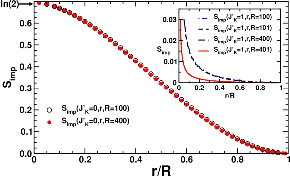
Figure 5: DMRG results using spin-inversion with $m=256$for $S_{\mathrm{imp}}(0,r,{R})$ for $\mathcal{R}$ even (${R}=100,400$). Results are shown for the $J_{1}-J_{2}$ spin chain model at $J_{2}^{c}$. Inset: DMRG results for $S_{\mathrm{imp}}(1,r,{R})$ for ${R}$ odd and even. Data for ${R}=100,101$ and ${R}=400,401$ are indistinguishable. $S_{{imp}}(1,r,{R})$ appears to vanish in the scaling limit $r\to\infty$ with $r/{R}$ held fixed.

We extracted an impurity part from $S_{U}$ by:

$$S_{\mathrm{imp}}(J^{\prime}_{K},r,{R})\equiv S_{U}(J^{\prime}_{K},r,{R})-S_{U}(1,r-1,{R}-1),\ r>1.$$ (3.34)

Note that we are subtracting the entanglement entropy of a chain where all couplings have unit strength and 1 site is removed. This corresponds to subtracting the entanglement entropy of the system without the impurity. It is important here that we do not subtract the entropy for the same values of $r$ and $R$ but with $J_{K}^{\prime}=0$ since, as we discuss below, entanglement with the impurity can survive, even in this limit, when $R$ is even, in the spin-singlet ground state. (See Fig. 5). This is related to the second subtlety that we encountered: a very strong dependence of $S_{\mathrm{imp}}$, as defined by Eq. (3.34), on the parity of $R$, even after subtracting off the part alternating in $r$. This is illustrated by some of our DMRG data shown in Fig. 6.

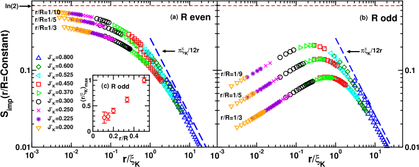
Figure 6: Universal scaling plot of $S_{\mathrm{imp}}$ for fixed $r/R$, (a) for $R\leq 102$ even, (b) for $R\leq 101$ odd. DMRG results with $m=256$ for the $J_{1}-J_{2}$ chain at $J^{c}_{2}$ for various couplings $J_{K}^{\prime}$. The lines marked $\pi\xi_{K}/(12r)$ are the FLT prediction: Eq. (3.39). (c): the location of the maximum, $(r/\xi_{K})_{\rm max}$, of $S_{\mathrm{imp}}$ for odd $R$, plotted versus $r/R$. Reprinted from  [7].

This figure tests the conjecture that the impurity entanglement entropy shows universal RG scaling behavior. We find that the data for the impurity entanglement entropy for various Kondo couplings can be collapsed onto scaling curves which depend only on the dimensionless ratios $r/\xi_{K}$, where $\xi_{K}$ is the Kondo length scale, and $r/R$. However, there are two different sets of curves depending on the parity of $R$. Note that the curves differ markedly for $r\ll\xi_{K}$ but elsewhere look similar. Indeed it looks likely, and presumably must be the case, that as $r/R\to 0$, the curves become identical for even and odd $R$. Focusing on the even $R$ curves, which seem close to the $r/R\to 0$ limit, the scaling curves seem to be approach a monotone decreasing function with the value $\ln 2$ at $r\ll\xi_{K}$ and zero for $r\gg\xi_{K}$. This is exactly what we would expect from the RG theory of the Kondo model and mirrors the $T$-dependence of the thermodynamic impurity entropy, reviewed in subsection (3.1). In particular, $\ln g=\ln 2$ at the short distance weak coupling fixed point, corresponding to a paramagnetic spin-1/2 impurity but $\ln g=0$ at the long distance strong coupling fixed point, corresponding to the spin being screened.

A qualitative understanding of the surprising difference between even and odd $R$ can be obtained using a “resonating valence bond” picture of the ground state of the $s=1/2$ Heisenberg antiferromagnetic chain [7]. Consider first even $R$. Any singlet state can be written as a linear superposition of products of singlet states formed by pairs of spins. Conventionally one draws a line or “valence bond” between pairs of spins contracted to a singlet, $(|\uparrow\downarrow>-|\downarrow\uparrow>)/\sqrt{2}$. It can easily be shown that by restricting to terms in which none of the lines cross we get a complete linearly independent set of singlet states for a S=1/2 chain. Furthermore, by adopting a convenient sign convention for valence bond states, it can be proven that all terms in the sum have non-negative coefficients. We may heuristically associate the impurity entanglement entropy with the valence bond originating from the impurity spin at site 1. If this spin forms a singlet with a spin at a site inside region $A$ (at a site with index $\leq r$) then we consider this not to contribute to the impurity entanglement entropy, $S_{\mathrm{imp}}$ of region $A$. On the other hand, if site 1 is paired with a site outside region $A$ (with index $>r$) then we consider it to contribute to $S_{\mathrm{imp}}$.

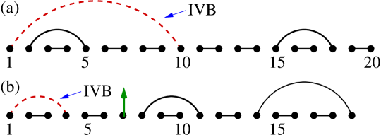
Figure 7: Typical impurity valence bond configurations for $R$ even (a) and $R$ odd (b). Note the unpaired spin on the $7^{\rm th}$ site in (b). Reprinted from [7].

The ground state is a sum over many valence bond configurations so we could imagine relating $S_{\mathrm{imp}}$ to the probability of this “impurity valence bond” (IVB) extending out of region $A$ [16, 7]. (See Fig. 7.) Similar ideas have been explored in [46]. As $J_{K}^{\prime}$ gets smaller, the IVB gets longer ranged. This follows because, in general, valence bonds tend to be nearest neighbor, or at least quite short range in order to take advantage of the nearest neighbor antiferromagnetic interactions. However, as $J_{K}^{\prime}$ gets weaker there is less and less energetic advantage in a short impurity valence bond. In the extreme case $J_{K}^{\prime}=0$ the impurity valence bond extends with significant probability over the entire chain. We expect that the typical length of this impurity valence bond should be $\xi_{K}$, the Kondo screening cloud size. This is a characteristic length scale, of order $v/T_{K}$, at which the effective Kondo coupling becomes of order one. In a metal, one heuristically imagines an electron in a quasi-bound state forming a singlet with the impurity spin with $\xi_{K}$ being the extent of the bound state wave-function. In the spin chain realization of the Kondo model this quasi bound state corresponds to the impurity valence bond. Thus the fact that $S_{\mathrm{imp}}$ starts to decrease when $r$ exceeds $\xi_{K}$ is very natural from this Kondo screening cloud viewpoint. Unfortunately, it seems extremely difficult to make this more than a heuristic argument. A problem is that the valence bond basis, while complete and linearly independent, is not an orthonormal basis. Although one could define a probability distribution for the length of the IVB it is hard to relate this to physical quantities such as the correlation length or the entanglement entropy. However, we can formally write:

$$S_{\mathrm{imp}}^{\mathrm{IVB}}=(1-p)\ln 2,$$ (3.35)

with $p$ the probability that the IVB connects the impurity spin to a spin in region $A$. This follows, since if the IVB does not cross the boundary between regions $A$ and $B$ its contribution to $S_{\mathrm{imp}}$ is obviously zero, on the other hand, if the IVB connects to a spin in region $B$ it will contribute a factor of $\ln(2)$. It is possible to be a little bit more quantitative using the recently introduced valence bond entropy [47, 48]. If one simply focuses on the IVB connecting the spin impurity with the rest of the system, we expect the probability $\cal{P}$ that the IVB has a length $r$ to decay like $\xi_{K}/r^{2}$ in the regime $r\gg\xi_{K}$, thus giving

$$S_{\mathrm{imp}}^{\mathrm{IVB}}(r)=\ln 2\left(1-\int_{1}^{r}{\cal{P}}{\rm{d}}r^{\prime}\right)\sim A\ln(2)\frac{\xi_{K}}{r}~{}~{}(r\gg\xi_{K}).$$ (3.36)

Such a $1/r^{2}$ behavior is expected for a pure system [49].

Now consider the case of odd $R$. The ground state now has a total spin of 1/2. We may again represent it by valence bonds but there are $(R-1)/2$ of them with one unpaired spin. This unpaired spin may or may not be the impurity spin. As $J_{K}^{\prime}$ gets weaker it becomes more and more likely that the impurity spin is unpaired. Clearly when $J_{K}^{\prime}=0$ the other $R-1$ spins form a singlet leaving the impurity in a paramagnetic state. In this limit, for odd $R$, $S_{\mathrm{imp}}$ is precisely zero, due to the way we have defined it. Numerically, we find that the maximum in $S_{\mathrm{imp}}$, for odd $R$, occurs at a value of $J_{K}^{\prime}$ such that $\xi_{K}\propto R$. This is due to trade-off between two competing effects. As we decrease $\xi_{K}$ from large values we increase the probability of having an IVB (i.e. of the impurity not being the unpaired spin). This tends to increase $S_{\mathrm{imp}}$. However, once $\xi_{K}$ becomes less than $R$, the shortening of the IVB with decreasing $\xi_{K}$ becomes important and decreases $S_{\mathrm{imp}}$. It is now clear that the limits $\xi_{K}\to\infty$ and $R\to\infty$ don’t commute. Taking $R\to\infty$ for any fixed $r$ and $\xi_{K}$ gives the same $S_{\mathrm{imp}}(r/\xi_{K})$ as occurs for even $R$: a monotone decreasing function. However, holding $R$ fixed and varying $\xi_{K}$ gives a maximum of $S_{\mathrm{imp}}$ in the vicinity of $\xi_{K}\approx R$. Again, this is largely a heuristic picture.

While we so far only have heuristic descriptions of $S_{\mathrm{imp}}$ when $\xi_{K}$ is of order $R$ and/or $r$, CFT methods can be used to calculate an analytic expression for $S_{\mathrm{imp}}$ in the opposite limit $\xi_{K}\ll r$ (for any ratio of $r/R$) [16, 7]. (Note that in this limit the dependence on the parity of $R$ disappears.) This calculation is based on doing perturbation theory for $S_{\mathrm{imp}}$ in the leading irrelevant operator at the strong coupling, infrared fixed point. In fact such perturbation theory is very powerful and very well-known for the Kondo effect, going under the name of Nozières local Fermi liquid theory (FLT). It has been used long ago to calculate the leading dependence at low temperature of thermodynamic and transport quantities. This approach can be based on the continuum limit field theory of Eq. (3.26). The infrared stable, strong coupling fixed point Hamiltonian does not contain the impurity spin since it is screened and breaking this singlet costs an energy of $O(T_{K})$. The low energy Hamiltonian at energy scales $\ll T_{K}$ only contains the continuum WZW fields. In this simple, spin-only model, the only effect of the Kondo interaction, once it has renormalized to strong coupling, is to switch the finite size spectrum of the WZW model between the $s=0$ and $s=1/2$ conformal tower, corresponding to removing one site. To perturb around this fixed point we must identify the leading irrelevant operator which we expect to appear as a boundary interaction at $r=0$ only. [It must be understood that this low energy theory is only valid at length scales large compared to $\xi_{K}$. We may think of the boundary interaction as being smeared over a distance of $O(\xi_{K})$ but this is effective the same as being right at the boundary, $r=0$ in the effective Hamiltonian.] The leading irrelevant boundary operator, which must have $SU(2)$ symmetry, is simply $\vec{J}_{L}^{2}(r=0)$. [Recall that the BC $\vec{J}_{L}(0)=\vec{J}_{R}(0)$ means there is only one boundary current operator.] Very fortunately, this leading irrelevant interaction is proportional to the bulk energy density, as we see from Eq. (3.29). Defining this energy density:

$${\cal H}_{s,L}(r)=(v/6\pi)\vec{J}_{L}\cdot\vec{J}_{L}$$ (3.37)

the leading irrelevant interaction at the infrared stable fixed point is conventionally written:

$$H_{int}=-(\pi\xi_{K}){\cal H}_{s,L}(0).$$ (3.38)

This can be taken as a precise definition of the crossover length scale $\xi_{K}$. The fact that $H_{int}$ can be written in terms of ${\cal H}_{s,L}$ is very convenient for calculating the leading perturbation to the entanglement entropy because we may simply take over the earlier results of Calabrese and Cardy. These imply the leading correction:

$$S_{\mathrm{imp}}\to\pi\xi_{K}/(12r),$$ (3.39)

representing first order perturbation theory in $\xi_{K}$, valid when $r\gg\xi_{K}$. This result is obtained for infinite $R$ but we may obtain the finite $R$ result by a standard conformal transformation:

$$S_{\mathrm{imp}}=\frac{\pi\xi_{K}}{12{R}}\left[1+\pi(1-\frac{r}{{R}})\cot(\frac{\pi r}{{R}})\right].$$ (3.40)

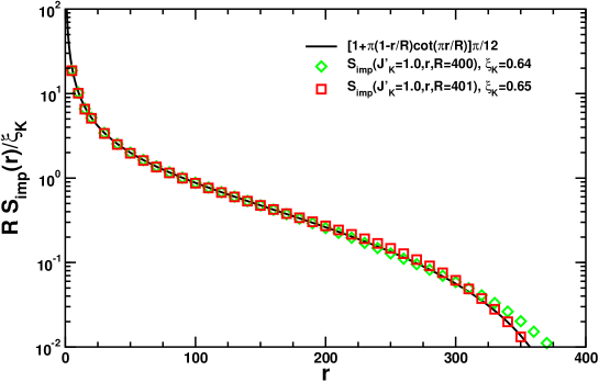
Figure 8: DMRG results with $m=256$ for the $J_{1}-J_{2}$ chain. $S_{imp}(J^{\prime}_{K}=1,r,{R})$ for ${R}=400,401$ with $J_{2}=J_{2}^{c}$ compared to the FLT prediction, Eq. (3.40).

We find that this formula fits our numerical data, for both even and odd $R$, extremely well as illustrated in Fig. 8. Note that there are essentially no free parameters in the fit except for $\xi_{K}$ which can be determined independently as a function of $J_{K}^{\prime}$ and is expected to behave exponentially at weak coupling:

$$\xi_{K}\propto\exp[1.38/J_{K}^{\prime}].$$ (3.41)

(The parameter, $1.38$ is not a fitting parameter but is rather determined from a careful mapping of the weak coupling of the end spin to the Kondo coupling in the usual fermion Kondo model.) This good fit of the CFT predictions to DMRG results on the spin chain version of the Kondo model is rather striking confirmation of the universality of entanglement entropy.

3.3 Topological entanglement entropy

We now consider a class of gapped 2D systems known as topological insulators. These occur most famously as models for the fractional quantum Hall effect although other experimentally relevant possibilities have been conjectured. The gapped excitations of these systems can exhibit non-abelian statistics and are currently of great interest as possible topological quantum computers. It is rather difficult to demonstrate numerically that a given microscopic model has a topological ground state of a given type. Recently, it was observed that this information can be extracted from the entanglement entropy. If we consider the entanglement entropy of a finite region inside a 2D insulator of infinite extent then we expect “area law” behavior:

$$S=\alpha R^{\prime}$$ (3.42)

where $R^{\prime}$ is the length of the perimeter of the region and $\alpha$ is a non-universal constant. However, it was recently shown [17, 18] that there is a sub-leading universal topological term in the entanglement entropy which is independent of the length and shape of the perimeter:

$$S=\alpha R^{\prime}-\ln{\cal D}.$$ (3.43)

To actually extract this term, it was proposed to divide the infinite 2D space into 3 or 4 imaginary finite regions and 1 infinite one and to calculate a sum and difference of various entanglement entropies so that the term $\propto R$ cancels. The connection of this term with the impurity entropy, $\ln g$ was suggested in [17]. (See also [18]). It was further elucidated in [50] using the connection of a 2D topological insulator with a 1D edge model. Consider for example a “quantum Hall bar”, a macroscopic sample of a topological insulator with edges. It is known that the electric current responsible for the Hall conductivity, $\sigma_{xy}$, flows around the edges only, in a clean sample, in a direction determined by the magnetic field direction, which is perpendicular to the plane. The low energy excitations on the edge correspond to a chiral CFT, meaning that the excitations are moving in only one direction. By considering a long thin hall bar, such as in Fig. (9) one can formally group together the right moving excitations on the upper edge and the left moving excitations on the lower edge to obtain a parity symmetric CFT. (As in all CFT’s the left and right moving sectors are decoupled.) This is a particularly convenient formulation if a constriction is created in the Hall bar, corresponding to a narrowing of the bar (usually imposed with gate voltages) at one point, as shown in Fig. (9). The constriction leads to “back-scattering” i.e. reflection of right-movers approaching the constriction on the upper edge into left-movers leaving it on the lower edge. Integrating out the gapped bulk modes, this can be described by a purely 1D parity symmetric field theory: a CFT with a local back-scattering interaction. In some situations, for example a simple CFT corresponding to spinless fermions with repulsive interactions, this back-scattering is a relevant interaction and can block all transport between left and right sides of the 1D system at low energies and long lengths. (This can be understood in terms of the boundary RG discussed in subsection 2.1). To make this connection more explicit let’s consider the case where the constriction has zero width in the $x$-direction and is parity invariant so that it acts only on the parity even channel of excitations. It is then possible to make a “folding transformation” mapping the 1D infinite system to a 1D semi-infinite system, $r\geq 0$ with the scatterer at $r=0$. The incoming parity even excitations are mapped to left movers and the outgoing parity even excitations to right movers. The back-scattering interaction becomes a boundary sine-Gordon interaction for the boson field corresponding to the parity even excitations. When the back-scattering is relevant it leads to an RG flow from Neumann to Dirichlet BC’s on the parity even boson. This is associated with a non-zero change in the impurity thermodynamic entropy, $\ln g$ which depends on the strength of the bulk excitations. In the original 2D model, we may think of the relevant constriction as effectively breaking the Hall bar into 2 pieces, each with its own chiral edge modes, as shown in Fig. (9).

Figure 9: A long thin Hall bar with a chiral edge current and a constriction. In sub-section 3.3 we let $R\to\infty$ and consider the entanglement entropy for the region of width $2r$ with the rest of the Hall bar. In subsection 3.4 we take $R$ finite and consider the entanglement of the left side of the entire system with the right side.

Again we may relate the impurity thermodynamic entropy to the impurity entanglement entropy. To do this, in the original 2D model, it is convenient to consider the entanglement of some region, $A$, containing the constriction and extending a distance $r$ on either side of it, with the rest of the infinite Hall bar. The corresponding entanglement entropy, in the 1D folded formulation can be decomposed into a sum of contributions from even and odd parity modes. Only the even parity part is affected by the constriction. The corresponding entanglement entropy for the even parity edge modes is:

$$S=\frac{1}{3}\ln\left(\frac{r}{a}\right)+\ln g+s_{1}$$ (3.44)

the standard result for a finite region in an infinite CFT with $c=1$ (eg. with periodic BC’s). Note that we have so far only considered the entanglement between region $A$ and the rest due to the gapless edge modes. We expect additional contributions from the bulk modes, $2\alpha w$, where $w$ is the width of the Hall bar and hence $2w$ is the length of the boundary of region $A$. Note that the extra term $(1/3)\ln r$ does not occur in the formulation of [17, 18] where the region $A$ does not include any physical boundaries and hence does not include any edge states.

Now consider the change in entanglement entropy for region $A$ with the rest, as we increase the length, $2r$, of region $A$. We then expect an RG flow from the clean Hall bar at small $r$ to a Hall bar broken in two at large $r$, with the crossover length scale determined by the strength of the back-scattering. From the viewpoint of the low energy 1D model, the change results from the RG flow of the BC and is given by the change in $\ln g$:

$$S_{\mathrm{IR}}-S_{\mathrm{UV}}=\ln g_{\mathrm{IR}}-\ln g_{\mathrm{UV}}.$$ (3.45)

[Note, in particular, that the $(1/3)\ln r$ term is the same in either perfectly transmitting or perfectly reflecting limits. In the first case it is the bulk 1D entanglement entropy for a region of length $2r$ in an infinite system. In the second it is twice the entanglement entropy for a region of length $r$ in a semi-infinite system.] On the other hand, from the viewpoint of topological entropy, the constriction has broken the Hall bar into two pieces, without effecting the length of the perimeter, separating region $A$ from the rest, $2w$. This is expected to double the topological entropy:

$$S_{\mathrm{IR}}-S_{\mathrm{UV}}=-\ln{\cal D},$$ (3.46)

since, in the infrared limit, we simply get twice the entanglement entropy of the Hall bar in the region $0<r^{\prime}<r$ with the region $r^{\prime}>r$, $2(\alpha w-\ln{\cal D})$ with zero entanglement between left and right sides, through the constriction. Thus we conclude that:

$$\ln{\cal D}=\ln g_{\mathrm{UV}}-\ln g_{\mathrm{IR}}.$$ (3.47)

Thus the topological entropy of a gapped 2D system is equal to the change in impurity entropy of the corresponding 1D gapless edge theory under a change in CIBC corresponding to breaking the system into two pieces. We note in passing that more generally, the local interactions associated with the constriction could lead to non-trivial boundary conditions not simply corresponding to perfect transmission or reflection. This would correspond to a different value of $g_{\mathrm{IR}}$ and probe other features of the topological insulator.

4 Bulk impurity effects

Another novel type of impurity entanglement entropy was studied in [19] and [20, 21]. We consider the same type of model as discussed in sub-section 3.3, a Luttinger liquid with a back-scatterer, considering the 1D formulation of the model. We now let the total system size $2R$ be finite with the back-scatterer in the centre. Rather than considering the entanglement of a central region containing the origin with the rest, these authors considered instead the entanglement entropy of the region to the left of the constriction with the region to the right. With no back-scattering this is:

$$S=\frac{c}{6}\ln\left(\frac{R}{a}\right).$$ (4.1)

With relevant backscattering, the 1D wire is effectively broken into two disconnected parts at long length scales so we might expect the entanglement entropy to vanish asymptotically. This was studied numerically using DMRG in a critical Heisenberg XXZ spin chain with Hamiltonian:

$$H=\sum_{j}J_{j}[(S^{x}_{j}S^{x}_{j+1}+S^{y}_{j}S^{y}_{j+1})+\Delta S^{z}_{j}S^{z}_{j+1}].$$ (4.2)

For uniform couplings, this model is in a gapless Luttinger liquid phase for $-1<\Delta\leq 1$. Here $J_{j}=1$ for all links except for one in the middle of the chain where it has the value $J_{\mathrm{imp}}<$ with $0<J_{\mathrm{imp}}<1$. This weakened link is a relevant perturbation for $\Delta>0$ but irrelevant for $\Delta<0$. The DMRG results were consistent with $S/\ln R$ going to zero at large $R$ for $0<\Delta\leq 1$ but going to $(1/6)$, the expected $c=1$ value, for $-1<\Delta<0$. A quantitative theory of the $R$-dependence has not yet been developed, as far as we know.

Properties of the impurity entanglement in the $s=1/2$ XX chain in a transverse field where the field strength is perturbed at a single central site have also been investigated [51, 52].

5 The alternating part of the entanglement entropy

5.1 Open boundary induced alternation

As discussed in Ref. [53, 22], in the case of AF spin chains with OBC, the von Neumann entropy can be written as a sum of two contributions:

$$S(r,R)=S_{\rm U}(r,R)+(-1)^{r}S_{\rm A}(r,R).$$ (5.1)

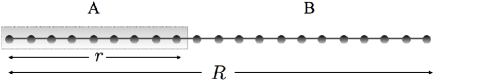
Figure 10: Schematic picture of a chain of total length $R$ with OBC. The system has been cut in two parts A and B. Sub-system A, of length $r$, includes one open end.

The uniform part $S_{\rm U}(r,R)$, in the case where the block of size $r$ contains one open end (depicted in Fig. 10), is given by the CFT result [11], Eq. (3.17):

$$S_{\rm U}(r,R)=\frac{c}{6}\ln\left[\frac{2R}{a\pi}\sin\left(\frac{\pi r}{R}\right)\right]+\ln g+s_{1}/2,$$ (5.2)

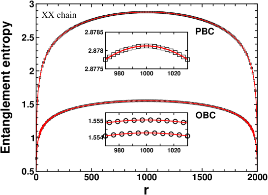
Figure 11: Results from ED of XX chains with $R=2000$ spins $1/2$. The von Neumann entropy $S(r,R=2000)$ is plotted vs the subsystem size $r$ for PBC (upper symbols) and OBC (lower symbols); the insets shows zooms around the chain center. The full lines are fits: Eq. (5.4) with $s_{1}=0.726$ for PBC. In the OBC case, uniform and staggered terms $\frac{0.055-(-1)^{r}0.25}{\frac{R}{\pi}\sin\left(\frac{\pi r}{R}\right)}$ have been added to Eq. (5.2). Reprinted from [22].

where $\ln g$ is the boundary entropy introduced in Ref. [10] and $s_{1}$ is a non-universal constant. $S(r,R)$ can be exactly computed numerically using either DMRG or exact diagonalization (ED). For the $S=1/2$ XXZ chain,

$${\cal{H}}_{\rm xxz}=J\sum_{r=1}^{R-1}\left(S_{r}^{x}S_{r+1}^{x}+S_{r}^{y}S_{r+1}^{y}+\Delta S_{r}^{z}S_{r+1}^{z}\right),$$ (5.3)

which is critical for $|\Delta|\leq 1$, there is a special point at $\Delta=0$ (XX point) where the spin chain is equivalent to free-fermions. There, one can numerically compute the von Neumann entropy [54] over for very large systems using ED, as shown in Fig. 11 both for PBC and OBC with $R=2000$ sites. For periodic chains, the numerical results for the entropy are very well described by the expression [11], Eq. (3.18):

$$S(r,R)=\frac{c}{3}\ln\left[\frac{R}{a\pi}\sin\left(\frac{\pi r}{R}\right)\right]+s_{1},$$ (5.4)

with $c=1$ and $s_{1}\simeq 0.726$ as predicted in Ref [55] for free-fermions. On the other hand for OBC, besides the uniform logarithmic increase Eq. (5.2), there are additional uniform and staggered terms which decay away from the boundary $(0.055-(-1)^{r}0.25)/\left[\frac{R}{\pi}\sin\left(\frac{\pi r}{R}\right)\right]$. Not predicted by CFT, the origin of the alternating term has been carefully investigated using ED and DMRG for critical XXZ chains in [22]. Such a phenomenon has also been observed in several other cases where DMRG were applied for open systems. As discussed above, in Ref. [20, 21] Peschel and co-workers, studying the effect of interface defects in critical spin chains, reported the observation of such oscillations. Fermions or bosons confined in 1D geometries with OBC are also affected by such a modulation, as reported for fermionic [56, 57, 58] and bosonic [59] Hubbard-like models.

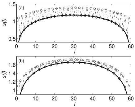
Figure 12: von Neumann entropy computed by DMRG for the $S=1$ bilinear-biquadratic model Eq. (5.5) on open chains for two critical points: (a) $\theta=-\pi/4$ and (b) $\theta=\pi/4$. Black lines are fits to the expression Eq. (5.2) with (a) $c=1.5$ and (b) $c=2$. Reprinted from [56].

An interesting example of critical spin chain is the $S=1$ bilinear-biquadratic model

$${\cal{H}}=\sum_{r=1}^{R-1}\left[\cos\theta\left(\vec{S}_{r}\cdot\vec{S}_{r+1}\right)+\sin\theta\left(\vec{S}_{r}\cdot\vec{S}_{r+1}\right)^{2}\right],$$ (5.5)

which displays conformally invariant critical points at $\theta=\pi/4$ with $c=2$ and at $\theta=-\pi/4$ with $c=3/2$. As studied by Legeza and co-workers [56], the dominant correlations at $k=\pi$ for $\theta=\pi/4$ and $k=2\pi/3$ for $\theta=-\pi/4$ show up in the von Neumann entropy as displayed in Fig. 12. However, a quantitative study of this boundary-induced term was not achieved in Ref [56] where the authors simply performed a fit to the expression Eq. (5.2) restricting to the lower points: $r=2p$ ($\theta=-\pi/4$) and $r=3p$ ($\theta=\pi/4$), with $p$ integer. Another interesting case has been studied with DMRG by Roux and collaborators [58] in the context of spin 3/2 fermionic cold atom with attractive interactions confined in a 1D optical lattice. They also found OBC-induced non-uniform features in the von Neumann entropy $S(r,R)$ with $2k_{F}$ oscillations that also appear in the local density and kinetic energy $t(r,R)$. Oscillations of $S(r,R)$ and $t(r,R)$ appear to be directly related as displayed in Fig. 13. Varying the parameters of the fermionic Hubbard model studied in this context [58], there is a critical point with $c=3/2$ which separates two phases with $c=1$. Imposing the non-uniform part of the von Neumann entropy to be directly proportional to the non-uniform part of the kinetic energy a good fit was obtained by Roux and collaborators with a clear jump in the central charge $c=1\to 3/2$ at the critical point [58].

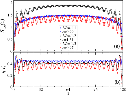
Figure 13: Von Neumann block entropy $S(x)$ for a block of size $x$ (a) and local kinetic energy $t(x)$ (b) around the critical point of a spin 3/2 fermionic Hubbard model with attractive interactions $U/t=-1.2$ for fixed $V/t=-2$ and $n=0.75$ with $L=128$. Fits using the oscillations of the local kinetic energy term (b) are quite accurate, allowing for the determination of the central charge $c$. Reprinted from [58].

5.2 Valence bond physics

Open boundary induced oscillations in the entanglement entropy appear to be a quite general phenomenon, as also observed in a valence bond physics framework [47, 48, 60, 61]. For SU(2) invariant spin systems, the $S_{\rm tot}=0$ sector can be studied by quantum Monte Carlo simulations in the valence bond basis [62]. In such a framework, one can define a Valence Bond Entropy which displays surprising similarities with the von Neumann entropy [47, 48, 60, 61].

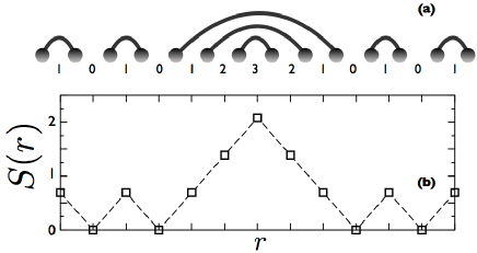
Figure 14: (a) Schematic picture for a particular valence bond state favored by OBC. The number of crossing bonds $N(r)$ is given. (b) Corresponding von Neuman entropy.

For random bond spin chains, Refael and Moore [46] achieved a very nice calculation of the von Neumann entropy, simply observing that for a single valence bond configuration (as depicted for instance in Fig. 14 (a)), the entropy is just given by $N(r)\times\ln 2$, where $N(r)$ is the number of singlet bonds crossing the interface between the two sub-systems. Such an idea was successfully checked numerically in the random bond case [63, 64, 47]. In the disorder free case, while the ground-state is a highly non-trivial superposition of a huge number of valence bond configurations, such a phenomenological approach appeared to be extremely useful to understand the oscillating features [22]. Indeed, since the translational invariance is explicitly broken by the open ends, there is tendency towards dimerization near the open edges. Such an effect can be computed very precisely (see below) but already at a qualitative level, this short-range singlet formation in the vicinity of open boundaries can be interpreted as an alternation of strong and weak bonds along the chain, thus leading to a similar alternation of $S(r,R)$. Indeed, the boundary spin at $r=1$ will have a strong tendency to form a singlet pair with its only partner on the right hand side. On the other hand the spin located at $r=2$ will be consequently less entangled with its right partner at $r=3$ since it already shares a strong entanglement with its left partner. A typical valence bon configuration favored by OBC is depicted in Fig. 14 (a) with the corresponding entropy (b). Such a qualitative interpretation in term of ”weak-strong” modulation is directly related to OBC induced Friedel-like oscillations that one can investigate in a more quantitative way, as we do now.

5.3 Entropy oscillation and dimerization for critical XXZ chains

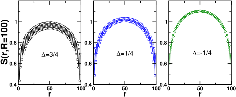
Figure 15: Von Neuman entropy of XXZ chains of lengths $R=100$ with OBC computed with DMRG for various anisotropies $\Delta$.

The alternating part $S_{A}(r,R)$ has been studied in Ref. [22] all along the critical regime of the XXZ chain $|\Delta|\leq 1$. DMRG results for $S(r,R)=S_{\rm U}(r,R)+(-1)^{r}S_{\rm A}(r,R)$ are shown in Fig. 15 for $R=100$ and various $\Delta$. One sees immediately that the oscillating part varies with $\Delta$ and decays faster in the ferromagnetic regime. More quantitatively, it was shown [22] that the alternating part $S_{A}(r,R)$ is directly proportional to the alternating term in the energy density. The energy density for XXZ spin chains:

$$\left\langle h_{r}\right\rangle=\langle S_{r}^{x}S_{r+1}^{x}+S_{r}^{y}S_{r+1}^{y}+\Delta S_{r}^{z}S_{r+1}^{z}\rangle$$ (5.6)

is uniform in periodic chains. On the other hand, an open end breaks translational invariance and there will be a slowly decaying alternating term or ”dimerization” in the energy density

$$\left\langle h_{r}\right\rangle=E_{U}(r)+(-1)^{r}E_{A}(r),$$ (5.7)

where $E_{A}(r)$ becomes nonzero near the boundary and decays slowly away from it. $E_{A}(r)$ is obtained by abelian bosonization modified by OBC [65]. In the critical region $\left|\Delta\right|\leq 1$, one gets [22, 7]

$$E_{A}(r,{{R}})\propto\frac{1}{[\frac{2{{R}}}{\pi}\sin(\frac{\pi r}{{{R}}})]^{K}},$$ (5.8)

where $K$ is the Luttinger liquid parameter defined as $K=\pi/(2(\pi-\cos^{-1}\Delta))$ so that $K=1$ for an XX spin chain, $K=1/2$ for the AF Heisenberg model, and $K\to\infty$ for the ferromagnetic Heisenberg case. Based on DMRG data obtained [22] on critical open chains of sizes $200\leq R\leq 1000$, we find a proportionality between $S_{A}$ and $E_{A}$. More precisely, plotting ${{S}}_{A}$ as a function of $-E_{A}$ for various values of the anisotropy $\Delta$ in Fig. 16, we find a linear relation ${{S}}_{A}=-\alpha E_{A}$ with a prefactor perfectly described by $\alpha=\mu/\sin\mu$, as shown in the inset of Fig. 16, with $\mu=\cos^{-1}\Delta$. We note that the velocity of excitations for the XXZ model is given by $v=\pi(\sin\mu)/(2\mu)$ so that we may write this relation as

$${S}_{A}=-(\pi a^{2}/2v)E_{A},$$ (5.9)

where we have introduced the lattice spacing, $a$, to make the entanglement entropy a dimensionless quantity ($E_{A}$ has dimensions of energy per unit length.).

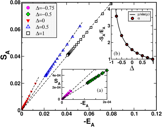
Figure 16: Linear behavior of the alternating part of the entanglement entropy, ${{S}}_{A}$ as a function of the alternating energy density, $-E_{A}$, both computed using DMRG on critical open XXZ chains of size $200\leq R\leq 1000$ for a few values of the anisotropy $\Delta$. Data from ED at $\Delta=0$ are also shown for $R=2000$. Dashed lines are linear fits of the form ${{S}}_{A}=-\alpha E_{A}$ (see text). The inset (a) is a zoom close to 0, showing data for $\Delta=-3/4$ and $-1/2$. The inset (b) shows the prefactor $\alpha$ vs $\Delta$ extracted from the numerical data (circles), for a larger set of values of $\Delta$, which is compared with $\pi/2v=\mu/\sin\mu$, $\mu=\cos^{-1}\Delta$. Reprinted from [22].

We emphasize that Eq. (5.9) even holds for the Heisenberg model (with a proportionality coefficient $\alpha=1$) where both $E_{A}$ and ${S}_{A}$ display the same logarithmic corrections. Indeed, at the Heisenberg point, $\Delta=1$, Eq. (5.8) will have some logarithmic corrections due to the presence of a marginally irrelevant coupling constant in the low energy Hamiltonian, leading to [22, 7] $E_{A}(r)\propto 1/[\sqrt{r}(\ln r)^{3/4}]$ in the limit $R\to\infty$. It is highly non-trivial to include both the log corrections and the finite size effects in $E_{A}(r,R)$. However, there is a simple result at $r=R/2$. Including the cubic term in the $\beta$-function for the marginal coupling constant, and other higher order corrections [66], this becomes:

$$E_{A}(\frac{R}{2},R)=a_{0}\frac{1+a_{2}/[\ln(R/a_{1})]^{2}}{\sqrt{R}[\ln(R/a_{1})+(1/2)\ln\ln(R/a_{1})]^{\frac{3}{4}}},$$ (5.10)

where $a_{0}$, $a_{1}$ and $a_{2}$ are constants. If one allows a frustrating second neighbor coupling $J_{2}$ in the chain, at $J_{2}^{c}=0.241167J$, this model is at the critical point between gapless and gapped spontaneously dimerized phase and the marginal coupling constant, and hence the log corrections are expected to vanish here. In both cases ($J_{2}=0$ and $J_{2}=J_{2}^{c}$), we found proportionality between $S_{A}$ and $E_{A}$, as shown in Fig. 17. The sum $E_{A}(R/2,R)+\alpha{S}_{A}(R/2,R)$ is found to rapidly decay as a power-law, with a power $\sim 2.5$ (see Fig. 17). Interestingly, for $J_{2}=0.241167$, again linearity is observed, but with a prefactor $\alpha\simeq 1.001689$ not related to the spin velocity, $v$, which we have determined to be $v\simeq 1.174(1)$ [45]. Hence, Eq. (5.9) does not hold in this case.

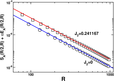
Figure 17: (a) Entanglement entropy $S(r)$ (black squares) and alternating part of the energy density $E_{A}(r)$ (open circles) computed with DMRG at $J_{2}^{c}$ for $R=200$ sites. The dashed line is Eq. (5.8). The uniform part of $S(r)$, obtained by taking $S(r)+(-1)^{r}\alpha E_{A}(r)$ with $\alpha=1.001699$, is represented by open squares. The best fit, shown by a red curve, is indicated on the plot. (b) Comparison between the alternating part ${{S}}_{A}$ and $E_{A}$ [Eq. (5.9)] from DMRG with $m=512$ states, for Heisenberg models. Power-law decay of ${S}_{A}(R/2,R)+\alpha E_{A}(R/2,R)$ drawn in a log-log plot, with $\alpha=1$ for the nearest neighbor chain ($J_{2}=0$) and $\alpha=1.00169$ at the critical second neighbor coupling $J_{2}=0.241167$. Lines are power-law fits: $\sim R^{-2.56}$ for $J_{2}=0.241167$ and $R^{-2.59}$ for $J_{2}=0$. (a) and (b) are respectively reprinted from [7] and [22].

We emphasize that this alternating term in ${S}(r,R)$ is universal and should not be regarded as a correction due to irrelevant operators. First of all, it is not a “correction”, since it is alternating. Secondly, it decays with the same power law as $E_{A}(r,R)$ which is seen to be a property of the fixed point, not the irrelevant operators. (However, for the Heisenberg model, $\Delta=1$, the log factor in $E_{A}(r,R)$ is due to the marginally irrelevant operator.) The presence of a universal alternating term in ${S}(r,R)$ is connected with the antiferromagnetic nature of the Hamiltonian (not appearing, for example, in the quantum Ising chain [15]) and does not seem to follow from the general CFT treatment in [11]. An analytic derivation of this phenomena remains an open problem.

5.4 Spin chain Kondo model

We now turn to the spin chain Kondo model Eq. (3.32). In previous sections, only the uniform part of the impurity part of the von Neumann entropy has been investigated. Here we focus on the alternating part which is also present for impurity problems. We want to isolate the impurity contribution in the alternating part of $S(r,R)$. Following our fundamental definition of

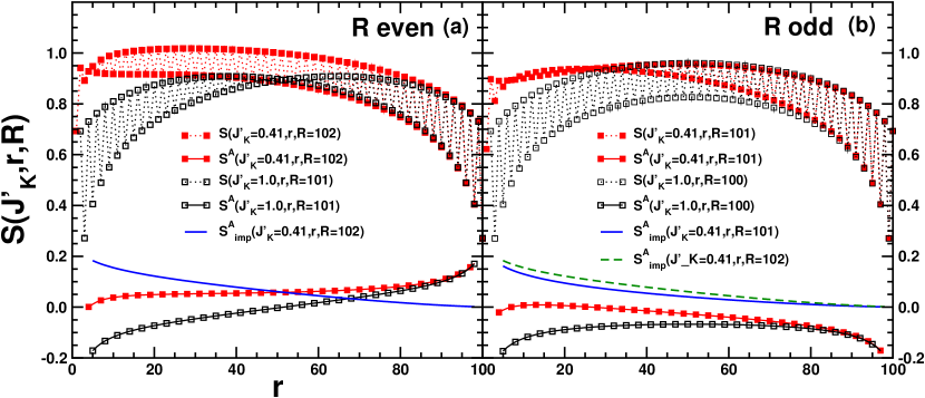
Figure 18: (a) DMRG results for the total entanglement entropy, $S(J^{\prime}_{K},r,R)$ for a 102 site spin chain at $J^{c}_{2}$, with a $J^{\prime}_{K}=0.41$ Kondo impurity ($\blacksquare$) along with $S(J^{\prime}_{K}=1,r-1,R-1)$ ($\square$). For both cases is the extracted alternating part shown along with the resulting $S^{A}_{imp}(J^{\prime}_{K}=0.41,r,R=102)$ for $R$ even. (b) DMRG results for the total entanglement entropy, $S(J^{\prime}_{K},r,R)$ for a 101 site spin chain at $J^{c}_{2}$, with a $J^{\prime}_{K}=0.41$ Kondo impurity ($\blacksquare$) along with $S(J^{\prime}_{K}=1,r-1,R-1)$ ($\square$). For both cases is the extracted alternating part shown along with the resulting $S^{A}_{imp}(J^{\prime}_{K}=0.41,r,R=101)$ for $R$ odd. For comparison we also show $S^{A}_{imp}(J^{\prime}_{K}=0.41,r,R=102)$ for $R$ even from panel (a) (dashed line). Reprinted from Ref. [7].

$S_{\mathrm{imp}}$, Eq. (3.34), it is also possible to define the alternating part of the impurity entanglement entropy:

$$S^{A}_{\mathrm{imp}}(J^{\prime}_{K},r,{{R}})\equiv S_{A}(J^{\prime}_{K},r,{{R}})-S_{A}(1,r-1,{{R}}-1).$$ (5.11)

As before, we have subtracted $S_{A}$ when the impurity is absent, in which case both $r$ and ${R}$ are reduced by one and the coupling at the end of this reduced chain, linking site $2$ to $3$ and $4$, has unit strength. Applying this definition to numerical data involves some subtleties. First of all $S^{A}$ is only defined up to an overall sign. Secondly, when calculating $S_{A}(1,r-1,{{R}}-1)$ we define this as $-S_{A}(1,r^{\prime},{{R}}^{\prime})$ with $R^{\prime}=R-1$ since the shift from $r$ to $r-1$ implies a sign change in the alternating part. For convenience we have therefore always exploited this degree of freedom to use a sign convention that makes the resulting $S^{A}_{\mathrm{imp}}$ positive in all cases. In Fig. 18 we show data for the total entanglement entropy along with the extracted alternating parts and the resulting $S^{A}_{imp}$ for both $R=102$ even and $R=101$ odd. As was the case for the uniform part of $S_{\mathrm{imp}}$ (Fig. 6) we do not observe any special features in $S^{A}_{\mathrm{imp}}(r)$ for fixed $R,J_{K}^{\prime}$ associated with the length scale $\xi_{K}$ and in all cases $S^{A}_{imp}$ decays monotonically with $r$. On the other hand, a possible scaling form for $S^{A}_{\mathrm{imp}}$ was suggested in Ref. [7]. For $J_{K}^{\prime}=1$ we have seen above that the alternating part of the entanglement entropy, $S_{A}$, is proportional to the alternating part in the energy, $E_{A}$ which, for $J_{2}=J_{2}^{c}$ can be written as follows: $E_{A}(r)=f(r/R)/\sqrt{r}$ for some scaling function $f$. A generalization of the above formula to the case $J_{K}^{\prime}\neq 1$ imply that $S^{A}_{\mathrm{imp}}\sqrt{r}$ should be a scaling function, $f(r/R,r/\xi_{K})$. DMRG results for $S^{A}_{\mathrm{imp}}\sqrt{r}$ for fixed $r/{R}$ are shown in Fig. 19 for a range of $J^{\prime}_{K}$ and ${R}$. The values for $\xi_{K}$ used to attempt the scaling are the ones previously used for the scaling of the uniform part (Fig. 6). Clearly the results for $S^{A}_{\mathrm{imp}}\sqrt{r}$ follow the expected scaling form.

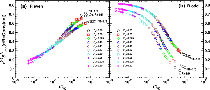
Figure 19: $\sqrt{r}S^{A}_{imp}$ for fixed $r/R$ and a range of couplings $J^{\prime}_{K}$ at $J_{2}^{c}$. (a) for $R$ even and (b) for $R$ odd. The values of $\xi_{K}$ used are obtained from the scaling of $S_{\mathrm{imp}}$ achieved in Fig. 6. DMRG results with $m=256$ states. Reprinted from Ref. [7].

6 Impurity entanglement in gapped spin chains

In previous sections the focus has largely been on work considering critical systems. However, impurity entanglement in systems with a gap, corresponding to massive field theories with a finite correlation length $\xi$, have also been considered. In this case the generalization of Eq. (1.2) to one dimensional systems with a gap becomes [11]:

$$S(r)\sim\frac{c}{6}\ln\left(\frac{\xi}{a}\right).$$ (6.1)

So far, mainly two models have been studied, $s=1$ chains [67, 68] at the AKLT point [69, 70] and $s=1/2$ $J_{1}-J_{2}$ chains [7] at the Majumdar-Ghosh point, $J_{2}=J_{1}/2$ [71]. While the $s=1$ spin chain at the AKLT point has a correlation length $\xi=1/\ln(3)$, the spin correlations in the $s=1/2$ chain at the MG point do not extend beyond nearest neighbor and the correlation length is effectively zero.

6.1 The $s=1$ ALKT chain

Boundary effects in the entanglement entropy of a $s=1$ chain was studied in [68] building on earlier work [67]. The model considered was the antiferromagnetic $s=1$ Heisenberg chain including a bi-quadratic term:

$$H=\sum_{j=-N_{l}+1}^{L+N_{r}-1}\left[{\vec{S}}_{j}\cdot{\vec{S}}_{j+1}+\frac{1}{3}({\vec{S}}_{j}\cdot{\vec{S}}_{j+1})^{2}\right].\ \ s=1.$$ (6.2)

For this special value of the bi-quadratic coupling, termed the AKLT point, the ground-state is known exactly [69, 70] and this fact was exploited to perform exact calculations of the entanglement entropy. The entanglement of a sub systems consisting of the central section of the chain, $1\ldots L$ with the remaining left and right parts of the chain was considered. Here $N_{l}$ and $N_{r}$ describe the size of the left and right parts of the system and it was shown [68] that the boundary effects in the entanglement entropy decay exponentially fast with $N_{l},N_{r}$ on a length scale equal to the correlation length $\xi=1/\ln(3)$. Hence, impurity effects in the entanglement impurity are in this case rather minor. In contrast, by considering a different subsystem impurity entanglement in the Majumdar Ghosh model can be rather pronounced.

The partial concurrence of the two effective $s=1/2$ spins at the end of an open $s=1$ chain has also been studied [30].

6.2 The Majumdar Ghosh Model

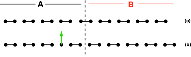
Figure 20: MG state divided in two regions $A$ and $B$. (a) The total number of site $R$ is even and the ground-state is a singlet. (b) ${\color[rgb]{0,1,0}\uparrow}$. Reprinted from [7]

At the special point $J_{2}=J_{1}/2$, often referred to as the Majumdar-Ghosh [72, 73, 71] (MG) point, the spin chain model Eq. (3.32) with $J_{K}^{\prime}=1$ is exactly solvable. The spin chain has a gap and for $R$ even, in the presence of periodic boundary conditions, a two-fold degenerate gound-state of nearest neighbor dimers either between sites $2n+1$ and $2n+2$ or $2n+2$ and $2n+3$, $n\geq 0$, with energy $E=-3RJ/8$. With open boundary conditions, for $R$ even, the ground-state is non-degenerate with dimers between sites $2n+1$ and $2n+2$, $n=0\ldots(R-1)/2$, and with the same energy as the periodic case, $E=-3RJ/8$. See Fig. 20(a). If one now instead considers $R$ odd, an exact form for the ground-state wave-function and energy is not known but a very precise variational form can be developed [74, 75, 76, 77, 78, 7, 79]. For $R$ odd it is natural to consider states of the following form:

$$|n\rangle\equiv|\overbrace{-\ \ldots\ -}^{n}\ \uparrow\ -\ \ldots\ -\rangle.$$ (6.3)

Here, $-$ indicates a singlet between site $r$ and $r+1$ and $n=0,\ldots N_{d}-1=(R-1)/2$ refers to the number of dimers to the left of the soliton, with $N_{d}$ the total number of dimers. See Fig. 20(b). Such states are often called thin soliton states (TS-states) because the soliton resides on a single site and is not ‘spread’ out over several sites as would have been the case if one had included states with valence bonds longer than between nearest neighbor sites. Note that the soliton only resides on the odd sites of the lattice, $r=1,3,\ldots,R$. It is important to realize that the TS-state as defined are not orthornormal and even though it is straight forward to form linear combinations $|m\rangle$ that are orthogonal [78, 79] through the transformation $|m=0\rangle\equiv|n=0\rangle,\ \ |m\rangle\equiv(2/\sqrt{3})\left[|n\rangle+(1/2)|n-1\rangle\right]\ m\geq 1$, one finds that for the purpose of calculating the entanglement this orthogonalization is less useful at the initial stage of calculating the entanglement entropy.

If only the ^⇑ state of the gound-state doublet for $R$ odd is considered one can write a thin soliton ansatz (TS-ansatz) for the ground-state wavefunction:

$$|\Psi_{TS}^{\Uparrow}\rangle\simeq\sum_{n=0}^{N_{d}}\psi^{sol}_{n}|n\rangle.$$ (6.4)

It can be shown that the restriction to the ^⇑ state is not important since any linear combination of the degenerate ^⇑ and ^⇓ states will yield the same entanglement entropy [7]. The components of the ground-state wavefunction, $\psi^{sol}_{n}$ can be obtained in a variational manner or through a simple analytical estimate [7]:

$$\psi^{sol}_{n}\simeq\sqrt{\frac{2}{N_{d}+2}}\sin\left(\frac{\pi(2n+2)}{{R}+3}\right).$$ (6.5)

With the $\psi^{sol}_{n}$ determined we can proceed with a calculation of the entanglement entropy. Due to the dimerization of the ground-state one sees that for $R$ even (and open boundary conditions) $S(r,R)$ simply oscilates with $r$ between $\ln(2)$ and 0 depending on whether $r$ is a site at the beginning or end of a dimer, respectively. With a $J_{K}^{\prime}\neq 1$ in Eq. (3.32) the entanglement is much richer and exact results are not available, however, very precise variational calculations [7] of $S(r,R)$ are possible. Let us first consider $R$ odd and $J_{K}^{\prime}=1$ with $r$ odd. We first divide the system in two parts ($A,B$) at $r$ and let $|\phi\rangle$ denote a basis for $1\ldots r$ and $|\psi\rangle$ a basis for $r+1..R$. We then have:

$$|\Psi_{TS}^{\Uparrow}\rangle=\sum_{i,j=0}^{3}C_{i,j}|\psi_{i}\rangle|\phi_{j}\rangle.$$ (6.6)

The above form follows since the system was divided in two parts at $r$ and since $r$ is odd. If the soliton is to the left of $r$ and since $r$ is odd the division between $A$ and $B$ will not ’cut’ a dimer. However, if the soliton is to the right of $r$ the division will cut a dimer and we effectively get an additional soliton at the end of the $A$ space leading to the following 3 separate cases for $|\psi_{i}\rangle$:

$$|\psi_{1}\rangle = \sum_{n=0}^{\frac{r-1}{2}}\psi^{sol}_{n}|\overbrace{-\ \ldots\ -}^{n}\ \uparrow\ -\ \ldots\ -\rangle$$

$$|\psi_{2}\rangle = |\overbrace{-\ -\ -\ \ldots\ -\ -\ -\ }^{\frac{r-1}{2}}\ \uparrow\rangle$$

$$|\psi_{3}\rangle = |\overbrace{-\ -\ -\ \ldots\ -\ -\ -\ }^{\frac{r-1}{2}}\ \downarrow\rangle.$$ (6.7)

With the corresponding definitions for $|\phi_{j}\rangle$:

$$|\phi_{1}\rangle = |\overbrace{-\ -\ -\ \ldots\ -\ -\ -\ }^{\frac{{R}-r}{2}}\rangle$$

$$|\phi_{2}\rangle = \sum_{n=0}^{\frac{{R}-r}{2}-1}\psi^{sol}_{\frac{r+1}{2}+n}|\downarrow\ \overbrace{-\ \ldots\ -}^{n}\ \uparrow\ -\ \ldots\ -\rangle$$

$$|\phi_{3}\rangle = \sum_{n=0}^{\frac{{R}-r}{2}-1}\psi^{sol}_{\frac{r+1}{2}+n}|\uparrow\ \overbrace{-\ \ldots\ -}^{n}\ \uparrow\ -\ \ldots\ -\rangle.$$ (6.8)

With these definitions it immediately follows that:

$$|\Psi_{TS}^{\Uparrow}\rangle=|\psi_{1}\rangle|\phi_{1}\rangle+\frac{1}{\sqrt{2}}\left[|\psi_{2}\rangle|\phi_{2}\rangle-|\psi_{3}\rangle|\phi_{3}\rangle\right].$$ (6.9)

from which the coefficients $C$ defined in Eq. (6.6) can be determined. The states $|\phi_{i}\rangle$ and $|\psi_{j}\rangle$ are clearly not orthonormal, however, by explicitly orthonormalizing the states $|\psi_{j}\rangle$ region $B$ can be traced out and the reduced density matrix $\rho$ for region $A$ determined It is straight forward to generalize this approach to the case where $r$ is even (and $R$ is odd with $J_{K}^{\prime}=1$).

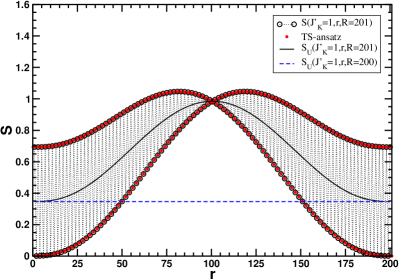
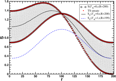
Figure 21: (a)DMRG results with$m=256$ for $S(J^{\prime}_{K}=1,r,{R}=201)$ for the spin-chain model with $J_{2}=1/2$ (MG model). The small solid circles represent the theoretical result obtained using the TS-ansatz. Also shown are the uniform parts $S_{U}(J^{\prime}_{K}=1,r,{R}=201)$ and $S_{U}(J^{\prime}_{K}=1,r,{R}=200)$ the difference of which is $S_{\mathrm{imp}}(J^{\prime}_{K}=1)$. (b)DMRG results with$m=256$ for $S(J^{\prime}_{K}=0,r,{R}=200)$ for the spin-chain model with $J_{2}=1/2$ (MG model). The small solid circles represent the theoretical result obtained using the TS-ansatz. Also shown are the uniform parts $S_{U}(J^{\prime}_{K}=0,r,{R}=200)$ and $S_{U}(J^{\prime}_{K}=1,r,{R}=199)$ the difference of which is $S_{\mathrm{imp}}(J^{\prime}_{K}=0)$.

Results from such a calculation is shown in Fig. 21(a) where they are compared to DMRG results. Excellent agreement is observed. For comparison, results for $S_{u}(J^{\prime}_{K}=1,r,{R}=201)$ and $S_{U}(J^{\prime}_{K}=1,r,{R}=200)$ are also shown in Fig. 21(a). The difference of these two uniform parts yields $S_{\mathrm{imp}}$. The influence of the impurity spin coupled with $J_{K}^{\prime}=1$ is clearly visible and extends over the entire range of $r$.

As already outlined in section 3.2, the entanglement of the impurity spin with the bulk of the chain is sizable (one might even say maximal) even when $J_{K}^{\prime}=0$. With some additional algebra it is possible to extend the thin-soliton approach also to this case [7] by considering a decoupled impurity entangled with a bulk chain of odd length $R-1$. Hence, the TS-ansatz can be applied to the bulk chain and precise variational results obtained. It is crucial to note that the impurity spin and the bulk chain form a singlet state even though their coupling, $J_{K}^{\prime}$, is zero. That is, we’re considering the $J_{K}^{\prime}\to 0$ limit of the entanglement entropy. Results obtained from the TS-ansatz are shown in Fig. 21(b) where they are compared to DMRG results obtained using spin-inversion. The DMRG calculations are performed on systems where the impurity spin is explicitly included resulting in a 4-fold degenerate ground-state consisting of a singlet and a triplet. The application of spin-inversion symmetry is therefore necessary in order to distinguish the singlet state of interest from the degenerate triplet state. The agreement between the numerical and variational results in Fig. 21(b) is excellent, the small discrepancies visible at a few values of $r$ are due to complications using spin-inversion [80] in the DMRG calculations specific to this value of $J_{2}$. For comparison, results for $S_{u}(J^{\prime}_{K}=0,r,{R}=200)$ and $S_{U}(J^{\prime}_{K}=1,r,{R}=199)$ are also shown in Fig. 21(b). The difference of these two uniform parts yields $S_{\mathrm{imp}}$ which is non-zero throughout the system.

Perhaps surprisingly, it is possible to obtain a much more intuitive picture and yet still very precise by simply assuming that the states $|\phi_{i}\rangle$ and $|\psi_{j}\rangle$ are orthogonal. With this assumption it is easy to see from Eq. (6.9) that the reduced density matrix for region $A$ (with $R$ odd) is simply:

$$\rho=\left(\begin{array}[]{ccc}p&0&0\cr 0&\frac{1-p}{2}&0\cr 0&0&\frac{1-p}{2}\cr\end{array}\right),\ r\ \mathrm{odd},\ \ \ \ \ \rho=\left(\begin{array}[]{ccc}1-p&0&0\cr 0&\frac{p}{2}&0\cr 0&0&\frac{p}{2}\cr\end{array}\right),\ r\ \mathrm{even}.$$ (6.10)

Here $p=\sum_{n=0}^{(r-1)/2}|\psi^{sol}_{n}|^{2}\sim r/R-\sin(2\pi r/R)/(2\pi)$ is the probability of finding the soliton in region $A$. From these expressions for $\rho$ the entanglement entropy can easily be evaluated. In order to calculate $S_{\mathrm{imp}}$ the uniform part of $S$ for an even length chain with $J_{K}^{\prime}=1$ is needed, but, as mentioned previously, this is simply $\ln(2)/2$ and it follows that:

$$S_{\mathrm{imp}}(J^{\prime}_{K}=1,r,{R})=-p\ln(p)-(1-p)\ln(1-p)\equiv S_{\mathrm{imp}}^{\mathrm{SPE}},{R}\ \mathrm{odd}.$$ (6.11)

In this case the impurity entanglement arises solely from the entanglement of a single particle (the soliton) that is present in the ground-state and one therefore refers to this contribution as the single particle entanglement, $S_{\mathrm{imp}}^{\mathrm{SPE}}$. See Fig. 22(b).

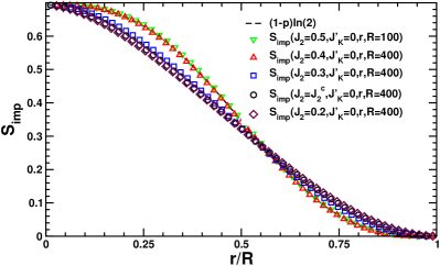
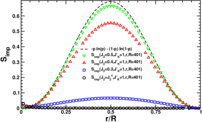
Figure 22: (a)DMRG results with$m=256$ for $S(J^{\prime}_{K}=0,r,{R}=400)$ for the spin-chain model with $J_{2}/J=0.2,J_{2}^{c},0.3,0.4,0.5$ shown along with the result for $S_{\mathrm{imp}}^{\mathrm{IVB}}=(1-p)\ln(2)$ with $p$ calculated at $J_{2}/J=0.5$ (dashed line). (b)DMRG results with$m=256$ for $S(J^{\prime}_{K}=1,r,{R}=401)$ for the spin-chain model with $J_{2}/J=J_{2}^{c},0.3,0.4,0.5$ . The dashed line represents $S_{\mathrm{imp}}^{\mathrm{SPE}}=-p\ln(p)-(1-p)\ln(1-p)$ with $p$ calculated at $J_{2}=J/2$. Reprinted from [7].

With more effort an analoguous calculation can be carried through for the case of $R$ even and $J_{K}^{\prime}=0$. One finds [7]:

$$S_{\mathrm{imp}}(J^{\prime}_{K}=0,r,{R})=(1-p)\ln(2)=S_{\mathrm{imp}}^{\mathrm{IVB}},{R}\ \mathrm{even}.$$ (6.12)

We see that in this case there is no contribution from the single particle entanglement as one would expect since there are no solitons (single particles) present in the ground-state. Instead, the impurity entanglement is given purely by the impurity valence bond impurity valence bond (IVB) (See section 3.2) where in the present case one identifies the probability that the IVB does not cross the boundary between regions $A$ and $B$ with the probability of finding a soliton in region $A$. See Fig. 22(a).

Some surprising observations can be found by performing numerical calculations of $S_{\mathrm{imp}}$ away from the MG point where the above variational calculations are quasi-exact. One finds [7]: (i) $S_{\mathrm{imp}}$ for both even and odd $R$ is non-zero over the entire range of $r$ and is not limited by the correlation length which is effectively zero. (ii) $S_{\mathrm{imp}}(J_{K}^{\prime}=0,r,R)$ for $R$ even changes only slightly when $J_{2}$ is decreased from $J_{2}=J/2$ to $J_{2}=J^{2}_{c}$ and for $J_{2}\leq J_{2}^{c}$ in the gapless phase it appears not to change at all with $J_{2}$. In all cases, $0\leq J_{2}\leq J/2$, does the IVB picture seem to correctly describe $S_{\mathrm{imp}}$. This is illustrated in Fig. 22(a). IT is perhaps surprising that the IVB picture works relatively well for $J_{2}<J_{2}^{c}$ where long-range valence bonds are present in the ground-state. (iii) $S_{\mathrm{imp}}(J_{K}^{\prime}=1,r,R)\sim S_{\mathrm{imp}}^{\mathrm{SPE}}$ for $R$ odd decreases rapidly with $J_{2}$ from $J/2$ to $J_{2}^{c}$ where it vanishes. For $J_{2}\leq J_{2}^{c}$ this part of the impurity entanglement is negligible. Hence, it seems likely that this fact is related to the system becoming gapless at $J_{2}^{c}$. This is illustrated in Fig. 22(b).

Finally we note that, the concurrence of the end spins in the dimerized $J_{1}-J_{2}$ $s=1/2$ model have been studied [30].

7 Conclusions

We have reviewed recent results related to the impurity contribution to the entanglement, $S_{\mathrm{imp}}$, arising from a quantum impurity or boundary. Most notably it has by now clearly been established that the entanglement can be dramatically changed by the presence of an impurity even in the case where the physical coupling to the impurity is zero. The role played by different boundary conditions in $1+1$ dimensional critical systems is well understood and in agreement with results from CFT. However, for the case of mixed boundary conditions (section 3.2) quantitative theory is not yet available and a detailed understanding of the $R$ dependence of bulk impurity effects (section 4) would be desirable. A consistent picture of the entanglement of a qubit with the environment as described by the spin-boson problem and the entanglement arising from Kondo impurities has been developed based on established theory of Kondo systems. A more heuristic picture of impurity entanglement in gapped (and to a certain extent also critical one dimensional systems) based on valence bond physics and matrix product states is emerging. Useful notions of single particle entanglement (SPE) and impurity valence bonds (IVB) have been introduced. Some details of this picture are still missing. As an example, how the single particle entanglement disappears as the system approaches criticality is still an open problem. Comparatively few results are available for quantum impourity entanglement in two (and higher) dimensional quantum systems and a detailed theory is still lacking.

References

- [1] J. von Neumann. Gött. Nachr., 273, 1927.
- [2] A. Wehrl. General properties of entropy. Rev. Mod. Phys., 50:221, 1978.
- [3] S. Y. Cho and R. H. McKenzie. Quantum entanglement in the two-impurity kondo model. Phys. Rev. A, 73:012109, 2006.
- [4] A. Kopp and K. Le Hur. Universal and measurable entanglement entropy in the spin-boson model. Physical Review Letters, 98(22):220401, 2007.
- [5] K. Le Hur, P. Doucet-Beaupre, and W. Hofstetter. Entanglement and criticality in quantum impurity systems. Physical Review Letters, 99(12):126801, 2007.
- [6] K. Le Hur. Entanglement entropy, decoherence, and quantum phase transitions of a dissipative two-level system. Annals of Physics, 323:2208–2240, 2007.
- [7] E. S. Sørensen, M.-S. Chang, N. Laflorencie, and I. Affleck. Quantum impurity entanglement. Journal of Statistical Mechanics: Theory and Experiment, 2007(08):P08003, 2007.
- [8] N. Andrei and C. Destri. Solution of the multichannel kondo problem. Phys. Rev. Lett., 52:364, 1984.
- [9] A.M. Tsvelik and P. B. Wiegmann. Exact solution of the multichannel kondo problem, scaling, and integrability. J. Stat. Phys., 38:125, 1985.
- [10] I. Affleck and A.W.W. Ludwig. Universal noninteger ground-state degeneracy in critical quantum systems. Phys. Rev. Lett., 67:161, 1991.
- [11] P. Calabrese and J. Cardy. Entanglement entropy and quantum field theory. J. Stat. Mech., page P06002, 2004.
- [12] J. Cardy and I. Peschel. Finite-size dependence of the free energy in two-dimensional critical systems. Nucl. Phys. B, 300:377, 1988.
- [13] C. Holzhey, F. Larsen, and F. Wilczek. Geometric and renormalized entropy in conformal field theory. Nucl. Phys. B, 424:443, 1994.
- [14] V. E. Korepin. Universality of entropy scaling in one dimensional gapless models. Phys. Rev. Lett., 92:096402, 2004.
- [15] H.-Q. Zhou, T. Barthel, J. Fjaerestad, and U. Schollwöck. Entanglement and boundary critical phenomena. Phys. Rev. A, 84:050305(R), 2006.
- [16] E. S. Sørensen, M.-S. Chang, N. Laflorencie, and I. Affleck. Impurity entanglement entropy and the kondo screening cloud. Journal of Statistical Mechanics: Theory and Experiment, 2007(01):L01001, 2007.
- [17] A. Kitaev and J. Preskill. Topological entanglement entropy. Phys. Rev. Lett., 96:110404, 2006.
- [18] M. Levin and X. G. Wen. Detecting topological order in a ground state wave function. Phys. Rev. Lett., 96:110405, 2006.
- [19] G. C. Levine. Entanglement entropy in a boundary impurity model. Phys. Rev. Lett., 93:226402, 2004.
- [20] I. Peschel. Entanglement entropy with interface defects. J. Phys. A, 38:4327, 2005.
- [21] J. Zhao, I. Peschel I, and X.Q. Wang. Critical entanglement of xxz heisenberg chains with defects. Phys. Rev. B, 73:024417, 2006.
- [22] N. Laflorencie, E. S. Sørensen, M.-S. Chang, and I. Affleck. Boundary effects in the critical scaling of entanglement entropy in 1d systems. Phys. Rev. Lett., 96:100603, 2006.
- [23] S. Bose. Quantum communication through an unmodulated spin chain. Phys. Rev. Lett., 91:207901, 2003.
- [24] M. Christandl, N. Datta, A. Ekert, and A. J. Landahl. Perfect state transfer in quantum spin networks. Phys. Rev. Lett., 92:187902, 2004.
- [25] Matthias Christandl, Nilanjana Datta, Tony C. Dorlas, Artur Ekert, Alastair Kay, and Andrew J. Landahl. Perfect transfer of arbitrary states in quantum spin networks. Physical Review A (Atomic, Molecular, and Optical Physics), 71(3):032312, 2005.
- [26] D. Burgarth and S. Bose. Perfect quantum state transfer with randomly coupled quantum chains. New J. Phys., 7:135, 2005.
- [27] D. Burgarth, V. Giovannetti, and S. Bose. Efficient and perfect state transfer in quantum chains. J. Phys. A, 38:6793, 2005.
- [28] A. Wójcik, T. Luczak, P. Kurzyński, A. Grudka, T. Gdala, and M. Bednarska. Unmodulated spin chains as universal quantum wires. Phys. Rev. A, 72:034303, 2005.
- [29] M. B. Plenio and F. L. Semião. High efficiency transfer of quantum information and multiparticle entanglement generation in translation-invariant quantum chains. New J. Phys., 7:73, 2005.
- [30] L. Campos Venuti, C. Degli Esposti Boschi, and M. Roncaglia. Long-distance entanglement in spin systems. Physical Review Letters, 96(24):247206, 2006.
- [31] L. Campos Venuti, C. Degli Esposti Boschi, and M. Roncaglia. Qubit teleportation and transfer across antiferromagnetic spin chains. Physical Review Letters, 99(6):060401, 2007.
- [32] T. Costi and R. H. McKenzie. Entanglement between a qubit and the environment in the spin-boson model. Phys. Rev. A, 68:034301, 2003.
- [33] E. S. Sørensen and I. Affleck. Scaling theory of the kondo screening cloud. Phys. Rev. B, 53:9153, 1996.
- [34] V. Barzykin and I. Affleck. The kondo screening cloud: What can we learn from perturbation theory. Phys. Rev. Lett., 76:4959, 1996.
- [35] V. Barzykin and I. Affleck. Screening cloud in the k-channel kondo model: Perturbative and large-k results. Phys. Rev. B, 57:432, 1998.
- [36] P. W. Anderson, G. Yuval, and D. R. Hamann. Exact results in the kondo problem. ii. scaling theory, qualitatively correct solution, and some new results on one-dimensional classical statistical models. Phys. Rev. B, 1(11):4464–4473, Jun 1970.
- [37] N. Andrei, K. Furuya, and J. H. Lowenstein. Solution of the kondo problem. Rev. Mod. Phys., 55(2):331–402, Apr 1983.
- [38] A. C. Hewson. The Kondo Problem to Heavy Fermions. Cambridge University Press, 2000.
- [39] Jr. A. T. Costa, S. Bose, and Y. Omar. Entanglement of two impurities through electron scattering. Physical Review Letters, 96(23):230501, 2006.
- [40] Peter Samuelsson and Claudio Verdozzi. Two-particle spin entanglement in magnetic anderson nanoclusters. Physical Review B (Condensed Matter and Materials Physics), 75(13):132405, 2007.
- [41] Ming-Liang Hu. Impurity entanglement in the open-ended heisenberg chains. Modern Phys. Lett., 29:2849–2855, 2008.
- [42] N. Andrei. Diagonalization of the kondo hamiltonian. Phys. Rev. Lett., 45:379, 1980.
- [43] P. B. Wiegmann. Exact solution of s-d exchange model at t = 0. JETP Lett., 31:364, 1980.
- [44] D. Friedan and A. Konechny. Boundary entropy of one-dimensional quantum systems at low temperature. Phys. Rev. Lett., 93:030402, 2004.
- [45] N. Laflorencie, E. S. Sørensen, and I. Affleck. The kondo effect in spin chains. Journal of Statistical Mechanics: Theory and Experiment, 2008(02):P02007 (31pp), 2008.
- [46] G. Refael and J. E. Moore. Entanglement entropy of random quantum critical points in one dimension. Phys. Rev. Lett., 93:260602, 2004.
- [47] F. Alet, S. Capponi, N. Laflorencie, and M. Mambrini. Valence bond entanglement entropy. Phys. Rev. Lett., 99:117204, 2007.
- [48] R. W. Chhajlany, P. Tomczak, and A. Wojcik. Topological estimator of block entanglement for heisenberg antiferromagnets. Phys. Rev. Lett., 99:167204, 2007.
- [49] F. Alet. Unpublished. Unpublished, 2009.
- [50] P. Fendley, M. P. A. Fisher, and C. Nayak. Topological entanglement entropy from the holographic partition function. J. Stat. Phys., 126:1111, 2007.
- [51] T. J. G. Apollaro and F. Plastina. Entanglement localization by a single defect in a spin chain. Physical Review A (Atomic, Molecular, and Optical Physics), 74(6):062316, 2006.
- [52] T. J. Apollaro, A. Cuccoli, A. Fubini, F. Plastina, and P. Verrucchi. Staggered magnetization and entanglement enhancement by magnetic impurities in a s = (1/2) spin chain. Physical Review A (Atomic, Molecular, and Optical Physics), 77(6):062314, 2008.
- [53] X. Wang. Boundary and impurity effects on the entanglement of heisenberg chains. Phys. Rev. E, 69:066118, 2004.
- [54] M.-C. Chung and I. Peschel. Density-matrix spectra of solvable fermionic systems. Phys. Rev. B, 64:064412, 2001.
- [55] B.-Q. Jin and V. E. Korepin. Quantum spin chain, toeplitz determinants and fisher-hartwig conjecture. J. Stat. Phys., 116:79, 2004.
- [56] Ö. Legeza, J. Sólyom, L. Tincani, and R. M. Noack. Entropic analysis of quantum phase transitions from uniform to spatially inhomogeneous phases. Phys. Rev. Lett., 99:087203, 2007.
- [57] E. Szirmai, Ö. Legeza, and J. Sólyom. Spatially nonuniform phases in the one-dimensional su(n) hubbard model for commensurate fillings. Phys. Rev. B, 77:045106, 2008.
- [58] G. Roux, S. Capponi, P. Lecheminant, and P. Azaria. Spin 3/2 fermions with attractive interactions in a one-dimensional optical lattice: phase diagrams, entanglement entropy, and the effect of the trap. Eur. Phys. J. B, 68:293, 2009.
- [59] A. Läuchli and C. Kollath. Spreading of correlations and entanglement after a quench in the one-dimensional bose-hubbard model. J. Stat. Mech., page P05018, 2008.
- [60] J. L. Jacobsen and H. Saleur. Exact valence bond entanglement entropy and probability distribution in the xxx spin chain and the potts model. Phys. Rev. Lett., 100:087205, 2008.
- [61] A. B. Kallin, I. González, M. B. Hastings, and R. G. Melko. Valence bond and von neumann entanglement entropy in heisenberg ladders. arXiv:0905.4286, 2009.
- [62] A. W. Sandvik. Ground state projection of quantum spin systems in the valence bond basis. Phys. Rev. Lett., 95:207203, 2005.
- [63] N. Laflorencie. Scaling of entanglement entropy in the random singlet phase. Phys. Rev. B, 72:140408(R), 2005.
- [64] J. A. Hoyos, A. P. Vieira, N. Laflorencie, and E. Miranda. Correlation amplitude and entanglement entropy in random spin chains. Phys. Rev. B, 76:174425, 2007.
- [65] S. W. Tsai and J. B. Marston. Density-matrix renormalization-group analysis of quantum critical points: I. quantum spin chains. Phys. Rev. B, 62:5546, 2000.
- [66] V. Barzykin and I. Affleck. Finite-size scaling for the s=1/2 heisenberg antiferromagnetic chain. J. Phys. A, 32:867, 1999.
- [67] H. Fan, V. Korepin, and V. Roychowdhury. Entanglement in a valence-bond solid state. Phys. Rev. Lett., 93:227203, 2004.
- [68] H. Fan, V. Korepin, V. Roychowdhury, and C. Hadley a S. Bose. Boundary effcts and two-site entanglement of the spin-1 valence-bond solid. Phys. Rev. B, 76:014428, 2007. cond-mat/0605133.
- [69] I. Affleck, T. Kennedy, E. H. Lieb, and H. Tasaki. Rigorous results on valence-bond ground states in antiferromagnets. Phys. Rev. Lett., 59(7):799–802, Aug 1987.
- [70] I. Affleck, T. Kennedy, E. H. Lieb, and H. Tasaki. Valence bond ground states in isotropic quantum antiferromagnets. Commun. Math. Phys., 115:477–528, 1988.
- [71] C. K. Majumdar. Antiferromagnetic model with known ground state. J. Phys. C, 3:911, 1970.
- [72] C. K. Majumdar and D. K. Ghosh. On next-nearest-neighbor interaction in linear chain i. J. Math. Phys., 10:1388, 1969.
- [73] C. K. Majumdar and D. K. Ghosh. On next-nearest-neighbor interaction in linear chain ii. J. Math. Phys., 10:1399, 1969.
- [74] B. S. Shastry and B. Sutherland. Excitation spectrum of a dimerized next-neighbor antiferromagnetic chain. Phys. Rev. Lett., 47:964, 1981.
- [75] W. J. Caspers and W. Magnus. Some exact excited states in a linear antiferromagnetic spin system. Phys. Lett. A, 88A:103, 1982.
- [76] W. J. Caspers, K. M. Emmett, and W. Magnus. The majumdar-ghosh chain. twofold ground state and elementary excitations. J. Phys. A, 17:2687, 1984.
- [77] E. S. Sørensen, I. Affleck, D. Augier, and D. Poilblanc. Soliton approach to spin-peierls antiferromagnets: Large-scale numerical results. Phys. Rev. B, 58:14701, 1998.
- [78] G. S. Uhrig, F. Schönfeld, M. Laukamp, and E. Dagotto. Unified quantum mechanical picture for confined spinons in dimerized and frustrated chains. Eur. Phys. J. B, 7:67–77, 1999.
- [79] R. L. Doretto and M. Vojta. Quantum magnets with weakly confined spinons: Multiple length scales and quantum impurities. arXiv:0904.0123, 2009.
- [80] E. S. Sørensen. Parity, precision and spin-inversion within the dmrg. J. Phys. Cond. Matt., 10:10655, 1998.