Hamiltonian flows with random-walk behavior
originating from zero-sum games and fictitious play

Abstract

In this paper we introduce Hamiltonian dynamics, inspired by zero-sum games (best response and fictitious play dynamics). Taking any piecewise affine Hamiltonian of a very simple form, the corresponding Hamiltonian vector field we obtain is discontinuous and multivalued. Nevertheless, somewhat surprisingly, the corresponding flow exists, is unique and continuous. We believe that these vector fields deserve attention, because it turns out that the resulting dynamics are rather different from those found in more classically defined Hamiltonian dynamics. The vector field is extremely simple: it is piecewise constant and so the flow $\phi_{t}$ piecewise a translation and in particular has no stationary points. Even so, the dynamics can be rather rich and complicated. For example, there exist Hamiltonian vector fields on ${\mathbb{R}}^{4}$ of this type with energy level sets homeomorphic to $S^{3}$ and so that the following holds. There exists a periodic orbit $\Gamma$ of the Hamiltonian flow so that, restricting to the level set containing $\Gamma$, the first return map $F$ to a two-dimensional section $Z$ transversal to $\Gamma$ at $x\in\Gamma$ acts as a random-walk: there exists a nested sequence of annuli $A_{n}$ in $Z$ (around $x$ so that $\cup A_{n}\cup\{x\}$ is a neighbourhood of $x$ in $Z$) shrinking geometrically to $x$ so that for each sequence $n(i)\geq 0$ with $|n(i+1)-n(i)|\leq 1$ there exists a point $z\in Z$ so that $F^{i}(z)\in A_{n(i)}$ for all $i\geq 0$. These Hamiltonian vector fields can also be used to obtain interesting continuous, area preserving, piecewise affine maps $R$ on certain two-dimensional polygons $S$, for which $R|\partial S=id$ so that $R$ has infinitely many periodic points (and conjecturally periodic orbits are dense on certain open subsets of $S$). In the last two sections of the paper we give some applications to game theory, and finish with posing a version of the Palis conjecture in the context of the class of non-smooth systems studied in this paper.

To Jacob Palis on his 70th birthday

Keywords: Hamiltonian systems, non-smooth dynamics, bifurcation, chaos, fictitious pay, learning process, replicator dynamics.
2000 MSC: 37J, 37N40, 37G, 34A36, 34A60, 91A20.

1 Introduction

In this paper we will introduce a rather unusual class of Hamiltonian systems. These are motivated by dynamics, usually referred to as ‘fictitious play’ and ‘best response dynamics’, associated to zero-sum games. These Hamiltonian systems differ from those that are considered traditionally, in that their orbits consist of piecewise straight lines and first return maps to certain planes are piecewise isometries. Specifically, the Hamiltonian systems we consider are continuous and piecewise affine, and defined by the Hamiltonian $H\colon\Sigma\times\Sigma\to{\mathbb{R}}$,

$$H(p,q)=\max_{p\in\Sigma}p^{\prime}\,{\mathcal{M}}\,q-\min_{q\in\Sigma}p^{\prime}\,{\mathcal{M}}\,q.$$

Here $\,{\mathcal{M}}\,$ is a $n\times n$ matrix, $p,q\in\Sigma$, the set of probability vectors in ${\mathbb{R}}^{n}$ and $p^{\prime}$ stands for the transpose of $p$. Note that $\max_{p\in\Sigma}\,p^{\prime}\,{\mathcal{M}}\,q$ is equal to the largest component(s) of the column vector $\,{\mathcal{M}}\,q$ and, similarly, $\min_{q\in\Sigma}\,p^{\prime}\,{\mathcal{M}}\,q$ is equal to the smallest component(s) of the row vector $p^{\prime}\,{\mathcal{M}}\,$. In other words,

$$H(p,q)=\max_{i}\,(\,{\mathcal{M}}\,q)_{i}-\min_{j}\,(p^{\prime}\,{\mathcal{M}}\,)_{j}\,\,,$$

where $(\,{\mathcal{M}}\,q)_{i}$ and $(p^{\prime}\,{\mathcal{M}}\,)_{j}$ stands for the $i$-th and $j$-th component of the vectors $\,{\mathcal{M}}\,q$ respectively $p^{\prime}\,{\mathcal{M}}\,$. Hence $H$ is continuous and piecewise affine ($H$ is affine outside some finite union of hyperplanes).

Definition (Completely mixed Nash equilibrium).

We say that a $n\times n$ matrix $\,{\mathcal{M}}\,$ has an completely mixed Nash equilibrium if there exist a unique ${\bar{p}},{\bar{q}}\in\Sigma$ so that all its components are strictly positive and so that ${\bar{p}}^{\prime}\,{\mathcal{M}}\,=\lambda\underline{1}$ and $\,{\mathcal{M}}\,{\bar{q}}=\mu\underline{1}$ for some $\lambda,\mu\in{\mathbb{R}}$ where $\underline{1}=(1\,1\,\dots\,1)\in{\mathbb{R}}^{n}$.

Let us denote the set of all $n\times n$ matrices by $L^{n}$ and the set of $n\times n$ matrices with a completely mixed Nash equilibrium by $LI^{n}$. Clearly $LI^{n}$ is an open subset of $L^{n}$.

Main Theorem.

There exists a subset $V\subset LI^{n}\times L^{n}$ which is open and dense and has full Lebesgue, so that for each pair of $n\times n$ matrices $(\,{\mathcal{M}}\,,A)\in V$ the following holds:

1. Any level set $H^{-1}(\varrho)$, for $\varrho>0$ small, is topologically a $2n-3$-sphere made up of hyperplanes. (Note that the dimension of $\Sigma\times\Sigma$ is $2n-2$.)

2. The Hamiltonian vector field $X_{H}$ associated to $H$ and the symplectic 2-form $\sum_{ij}a_{ij}dp_{i}\wedge dq_{j}$ (where $(a_{ij})$ are the coefficients of the matrix $A$) is piecewise constant and set-valued in codimension-one sets.

3. Correspondingly, we have a differential inclusion

   $$(\dfrac{dp}{dt},\dfrac{dq}{dt})\in X_{H}(p,q)$$

   where the right hand side is set-valued and $(p,q)\mapsto X_{H}(p,q)$ is piecewise constant.

4. The differential inclusion induces a unique continuous flow on $H^{-1}(\varrho)$ (for each $\varrho>0$ fixed and small) which is piecewise a translation flow. The flow has no stationary point.

5. First return maps between hyperplanes are piecewise affine maps.

Although we are dealing with a differential inclusion, solutions are unique, and define a continuous flow! Moreover, although these Hamiltonian vector fields are very simple in that they are piecewise constant, they generate surprisingly rich dynamics. Let us illustrate this by describing some interesting properties.

1.1 Examples with interesting properties

The first of property shows that many of these Hamiltonian vector fields induce continuous area-preserving piecewise affine maps $R$ on polygons $S$ in ${\mathbb{R}}^{2}$ so that $R=id$ on $\partial S$ and so that $R$ has infinitely many periodic orbits. We conjecture that periodic orbits are dense in open subsets of $S$. To construct maps of this type by ‘hand’ seems not so easy.

Examples having interesting first return maps.

There exists an open set of matrices $(\,{\mathcal{M}}\,,A)\in LI^{3}\times L^{3}$ so that for each corresponding Hamiltonian vector field $X_{H}$ there exists a topological disc $S$ consisting of four triangles (which are embedded in ${\mathbb{R}}^{4}$), see Figure 1, so that the first return map $R$ to $S$ of the flow of $X_{H}$ has the following properties:

1. $R\colon S\to S$ is area-preserving (w.r.t. Lebesgue measure), continuous and piecewise affine;

2. $R=id$ on $\partial S$;

3. $R$ has infinitely many periodic orbits of saddle-type.

....................................................................................................................................................................................................................................................................................................................................................................................................................................................................................................................................................................................................................................................................................................................................................................................................................................................................................................................................................................................................................................................................................................................................................................................................................................................................................................................

Figure 1: The topological disc $S$ consisting of four triangles.

Conjecture.

Let $R\colon S\to S$ be as in the previous set of examples. Then there exists a compact set $K\subset S$ so that the following properties hold.

• $K$ is either empty or consists of two regions bounded by two disjoint ellipses in $S$.

• If $K$ is non-empty, then $R$ permutes the two components of $K$. Moreover, $R^{2}|K$ is linearly conjugate to a rotation.

• Periodic orbits are dense in $S\setminus K$.

• There exists a dense orbit in $S\setminus K$ and $R$ is ergodic on $S\setminus K$.

Simulations give dynamics as in Figure 7. Although ‘typical’ orbits seem to be dense outside the two elliptic regions, the mechanism could be rather different from that of Arnol’d diffusion in classical smooth area preserving maps, see [1].

Another difference with classical dynamical systems is that invariant manifolds associated to a periodic orbit $\Gamma$ of the flow can be rather strange. For a smooth system one expects that all orbits near $\Gamma$ approach $\Gamma$ (either in forward or backward time) with some rate $\mu$ where $\mu$ is one of the multipliers of the linearization of a first return map along $\Gamma$. So only a finite number of rates is possible. Here the situation is totally different:

Example having random walk-like behaviour.

There exists an open set of matrices $(\,{\mathcal{M}}\,,A)\in LI^{3}\times L^{3}$ so that for the corresponding Hamiltonian vector field there exists a periodic orbit $\Gamma$ so that the stable manifold $W^{\tau}(\Gamma)$ of speed $\tau$ is non-empty for each $\tau\approx 0$.

So for each $\tau\approx 0$ there exist an initial condition $(p,q)$ so that

$$d(\phi_{t}(p,q),\Gamma)\approx e^{\tau t}\quad\left\{\begin{array}[]{ll}\mbox{ as }t\to\infty&\mbox{ when }\tau<0,\\ \mbox{ as }t\to-\infty&\mbox{ when }\tau>0.\end{array}\right.$$

In Section 7 we will explain this in more detail, and relate it to random-walk like behaviour.

1.2 Relationship to game theory

In the last section of this paper we will show how the previous set-up is related to game theory. However, let us state here already the following:

Second Main Theorem.

There exists a subset $W\subset LI^{n}$ which is open and dense and has full Lebesgue, so that for each pair of $n\times n$ matrix $\,{\mathcal{M}}\,\in W$ the following holds:

1. $({\bar{p}},{\bar{q}})\in\Sigma\times\Sigma$ is the unique Nash equilibrium of the zero-sum game best response dynamics

   $$\dfrac{dp}{dt}\in{\mathcal{B}\!\mathcal{R}\!}_{p}(q)-p,\dfrac{dq}{dt}\in{\mathcal{B}\!\mathcal{R}\!}_{q}(p)-q.$$ (1.1)

   associated to $\,{\mathcal{M}}\,$. Here ${\mathcal{B}\!\mathcal{R}\!}_{p}(q):=\operatorname*{arg\,max}_{p\in\Sigma}p^{\prime}\,{\mathcal{M}}\,q$ and $BR_{q}(p):=\operatorname*{arg\,min}_{q\in\Sigma}\,p^{\prime}\,{\mathcal{M}}\,q$.

2. The flow $\phi_{t}$ associated to this differential inclusion exists, is unique and continuous outside $({\bar{p}},{\bar{q}})$.

3. For each $\varrho>0$ small, each half-ray through $({\bar{p}},{\bar{q}})$ intersects $H^{-1}(\varrho)$ in a unique point. Let $\pi\colon(\Sigma\times\Sigma)\setminus\{({\bar{p}},{\bar{q}})\}\to H^{-1}(\varrho)$ be the corresponding continuous map. Then $\pi\circ\phi_{t}$ is the flow on $H^{-1}(\varrho)$ of a Hamiltonian vector field corresponding to $H$ and the symplectic form $\sum_{ij}a_{ij}dp_{i}\wedge dq_{j}$ where $(a_{ij})$ are the coefficient of the matrix $A:=\,{\mathcal{M}}\,$.

In fact, we will prove this result for a more general differential inclusion, see equation (4.12).

1.3 Relationship with other papers

Before describing these results in more detail, let us give a bit of background to the result of this paper and how it relates to the literature.

This study grew out of research into the best response dynamics (1.1) associated to two player games. This differential inclusion, or rather the differential inclusion

$$\dfrac{dp}{dt}\in\dfrac{1}{t}({\mathcal{B}\!\mathcal{R}\!}_{p}(q)-p),\dfrac{dq}{dt}\in\dfrac{1}{t}({\mathcal{B}\!\mathcal{R}\!}_{q}(p)-q).$$ (1.2)

was introduced in the late 1940’s by Brown [4] to describe a mechanism in which two players could ‘learn to play a Nash equilibrium’, and since then usually is referred to as fictitious play dynamics. Note that the orbits of (1.1) and (1.2) are the same up to time reparametrization and that their right hand side is piecewise affine (and multivalued in places). It the early 50’s Robinson [18] showed that the solutions of these differential inclusions converge to the set of Nash equilibria of the game. One can also define the corresponding differential inclusion for non-zero games, see Section 8. However, in the 60’s Shapley [20] showed that in that case these equations can have periodic attractors. Shapley’s example is extremely well-known in the very extensive literature on fictitious games, for references see for example [21] and for a discussion on the relationship of fictitious play and learning, see [7]. In the first of a sequence of papers ([21] and [22]), we considered a one-parameter family of games, which includes Shapley’s classical example, and analysed how Shapley’s periodic orbit bifurcates and how eventually other ‘simple’ periodic orbits are created In the second paper we study the dynamics of these games in much more detail, and how one can have ‘chaotic choice of strategies’ for the players. One of the ideas in that paper is to study the dynamics induced by projecting orbits onto the boundary of the space. In numerical studies, we observed (many years ago) that, in the zero-sum case, this induced dynamics behaves similarly to that of an area preserving flow. The present paper explains this observation.

In [22] we observed that the transition map associated to differential inclusion between hyperplanes is a composition of piecewise projective maps. In fact, as we show in this paper in the present case the transition map is continuous, volume preserving and piecewise affine. In particular, we obtain a family of continuous, piecewise affine, area preserving maps of a polygon in the plane with rather interesting dynamics. This connects this paper with an exciting body of work on piecewise isometries (with papers by R. Adler, P.Ashwin, M. Boshernitzan, A. Goetz, B. Kichens, T. Nowicki, A. Quas, C. Tresser and many others). Most of these papers deal with piecewise continuous maps, while the maps we encounter are continuous.

Another loose connection of our work is to that of the huge and very active field of translation flows (associated to interval exchange transformations, translation surfaces and Teichmüller flows) (with recent papers by A. Avila, Y. Cheung, A. Eskin, G. Forni, P. Hubert, H. Masur, C. McMullen, M. Viana, J-C. Yoccoz, A. Zorich and many many others). But of course our flow does not act on a surface with a hyperbolic metric, and so this connection seems not very helpful.

1.4 Relationship with the literature on non-smooth dynamical systems

We should point out that there are many results on nonsmooth dynamical systems. Most of these are motivated by mechanical systems with ‘dry friction’, ‘sliding’, ‘impact’ and so on. As the number of workers in this field is enormous, we just refer to the recent survey of M. di Bernardo et al [6] and the monograph by M. Kunze [12]. Of course our paper is very much related to this work, although the motivation and the result seem to be of a different nature from what can be found in those papers.

What our results have in common with many of the models in this literature, is that we are dealing with a differential inclusion $x^{\prime}\in f(x)$ where $f(x)$ is discontinuous and multi-valued in some hyperplanes. Our paper deals with a situation in which we also study differential inclusions but for which the flow exists, is unique and continuous. Moreover, the global dynamics around certain periodic orbits can be extremely complicated (much more so than would be possible in the smooth case). This behaviour is described in Theorem 7.1. We believe that this behaviour has not been observed before.

1.5 The organization of this paper

In Section 2 and 3 we discuss why level sets of $H$ are spheres and how to compute the Hamiltonian vector field $X_{H}$. In Section 4 we show that a related (set-valued) vector field has a continuous flow. In Section 5, we show this implies that the flow of the original Hamiltonian vector field is continuous. In Section 7.1 we will discuss some examples. Finally, in Section 8 we relate these results to dynamics associated to game theory (the so-called best response and fictitious play dynamics). We should emphasize that this paper does not include the proofs related to the examples for which random walk behaviour is shown. We describe these results briefly in Section 7.1, but for a detailed analysis see [22].

This paper requires no knowledge of game theory.

1.6 Notation and terminology

If $b_{1},\dots,b_{k}\in{\mathbb{R}}^{n}$ then we will denote by $<b_{1},\dots,b_{k}>$ the space spanned by these vectors and $[b_{1},\dots,b_{k}]$ the space of convex combinations of these points. We also sometimes refer to the subspace associated to $[b_{1},\dots,b_{k}]$: this is the smallest affine space containing $[b_{1},\dots,b_{k}]$. All vectors we consider are column vectors. If $p\in{\mathbb{R}}^{n}$ then $p^{\prime}$ always denotes the corresponding row vector. The transpose of a matrix $M$ is denoted by $M^{\prime}$.

2 $H$ and the best response functions

Let $n,m$ be positive integers and consider $H\colon\Sigma_{p}\times\Sigma_{q}\to{\mathbb{R}}$ of the form

$$H(p,q)=\max_{p\in\Sigma}p^{\prime}\,{\mathcal{M}}\,q-\min_{q\in\Sigma}p^{\prime}\,{\mathcal{M}}\,q,$$ (2.3)

where $\Sigma_{p}$ and $\Sigma_{q}$ are the set of probability vectors in ${\mathbb{R}}^{m}$ resp. ${\mathbb{R}}^{n}$ and $\,{\mathcal{M}}\,$ is a $m\times n$ matrix. We will denote by $e_{1}^{p},e_{2}^{p},\dots,e_{m}^{p}$ the unit vectors in $\Sigma_{p}$ and by $e_{1}^{q},e_{2}^{q},\dots,e_{n}^{q}$ the unit vectors in $\Sigma_{q}$. Often we will consider the case that $m=n$ and then write $\Sigma=\Sigma_{p}=\Sigma_{q}$. We will denote the subspace spanned by $\Sigma_{p}$ and $\Sigma_{q}$ by $\hat{\Sigma}_{p}$ and $\hat{\Sigma}_{q}$ and their tangent spaces by $T\Sigma_{p}$ and $T\Sigma_{q}$.

One can also write

$$H(p,q)=({\mathcal{B}\!\mathcal{R}\!}_{p}(q))^{\prime}\,{\mathcal{M}}\,q-p^{\prime}\,{\mathcal{M}}\,{\mathcal{B}\!\mathcal{R}\!}_{q}(p).$$ (2.4)

where ${\mathcal{B}\!\mathcal{R}\!}_{p}\colon{\mathbb{R}}^{n}\to\Sigma_{p}$ and ${\mathcal{B}\!\mathcal{R}\!}_{q}\colon{\mathbb{R}}^{m}\to\Sigma_{q}$ are defined by

$${\mathcal{B}\!\mathcal{R}\!}_{p}(q):=\operatorname*{arg\,max}_{p\in\Sigma_{p}}p^{\prime}\,{\mathcal{M}}\,q\,\,\mbox{ and }\,\,{\mathcal{B}\!\mathcal{R}\!}_{q}(p):=\operatorname*{arg\,min}_{q\in\Sigma_{q}}\,p^{\prime}\,{\mathcal{M}}\,q.$$ (2.5)

Due to their game-theoretic interpretation, which we will discuss in Section 8, ${\mathcal{B}\!\mathcal{R}\!}_{p}$ and ${\mathcal{B}\!\mathcal{R}\!}_{q}$ are called best response functions. Note that ${\mathcal{B}\!\mathcal{R}\!}_{p}$ and ${\mathcal{B}\!\mathcal{R}\!}_{q}$ are in actual fact set-valued, because ${\mathcal{B}\!\mathcal{R}\!}_{p}(q)=[e_{i_{1}}^{p},\dots,e_{i_{k}}^{p}]$ iff $i_{1},\dots,i_{k}$ are the largest components of $\,{\mathcal{M}}\,q$. Similarly, ${\mathcal{B}\!\mathcal{R}\!}_{q}(p)$ is equal to the convex combination of unit vectors corresponding to the smallest components of $p\,{\mathcal{M}}\,$. It follows that

$${\mathbb{R}}^{n}\ni q\mapsto{\mathcal{B}\!\mathcal{R}\!}_{p}(q)\in\Sigma_{p}\mbox{ and }{\mathbb{R}}^{m}\ni p\mapsto{\mathcal{B}\!\mathcal{R}\!}_{q}(p)\in\Sigma_{q}$$

are set-valued and upper semi-continuous. For example, when $m=n=2$ and $\,{\mathcal{M}}\,$ is the $2\times 2$ identity matrix, then we can write the probability vectors $p,q$ in the form $p=(p_{1},1-p_{1})$ and $q=(q_{1},1-q_{1})$, identify $\Sigma\times\Sigma=[0,1]\times[0,1]$ and we get $H(p,q)=\max(|q_{1}|,|q_{2}|)-\min(|p_{1}|,|p_{2}|)$. Moreover ${\mathcal{B}\!\mathcal{R}\!}_{p}(q)=e_{1}^{p}$ when $q_{1}>1/2$, ${\mathcal{B}\!\mathcal{R}\!}_{p}(q)=e_{2}^{p}$ when $q_{1}<1/2$ and ${\mathcal{B}\!\mathcal{R}\!}_{p}(q)=\Sigma_{p}$ when $q_{1}=1/2$. When $m=n=3$ and $\,{\mathcal{M}}\,$ is the $3\times 3$ identity matrix, then $H(p,q)=\max_{i}\,q_{i}-\min_{j}\,p_{j}$ and ${\mathcal{B}\!\mathcal{R}\!}_{p}$ and ${\mathcal{B}\!\mathcal{R}\!}_{q}$ are shown in Figure 2 (on the right).

......................................................................................................................................................................................................................................................................................................................................................................................................................................................................................................................................................................................................................................................................................................................................................................................................................................................................................................................................................................$\Sigma_{q}$$\Sigma_{p}$$e_{1}^{q}$$e_{2}^{q}$$e_{2}^{p}$$e_{1}^{p}$$(e_{2}^{p},e_{2}^{q})$$(e_{1}^{p},e_{2}^{q})$$(e_{1}^{p},e_{1}^{q})$$(e_{2}^{p},e_{1}^{q})$.............................................................................................................................................................................................................................................................................................................................................................................................................................................................................................................................................................................................................................................................................................................$e^{q}_{1}$$e^{q}_{2}$$e^{q}_{3}$$e_{1}^{p}$$e_{3}^{p}$$e_{2}^{p}$.................................................................................................................................................................................................................................................................................................................................................................................................................................................................................................................................................................................................................................................................................................................................................................................................................$e^{p}_{1}$$e^{p}_{2}$$e^{p}_{3}$$e_{2}^{q}$$e_{1}^{q}$$e_{3}^{q}$

Figure 2: On the left a level set of $H$ (drawn in dots), where we consider the case that $n=2$, take $\,{\mathcal{M}}\,$ the $2\times 2$ identity matrix and identify $\Sigma\times\Sigma=[0,1]\times[0,1]$. The values of $({\mathcal{B}\!\mathcal{R}\!}_{q}(p),{\mathcal{B}\!\mathcal{R}\!}_{p}(q))$ are also shown. In the right two figures the case where $m=n=3$, $\,{\mathcal{M}}\,=id$ is considered: level sets of $\max|q_{i}|$ and $\min|p_{i}|$ are drawn inside the simplexes $\Sigma_{p}$ and $\Sigma_{q}$. The values of ${\mathcal{B}\!\mathcal{R}\!}_{q}(p)$ and ${\mathcal{B}\!\mathcal{R}\!}_{p}(q)$ are also shown.

Definition 2.1 (Nash equilibrium).

We call $({\bar{p}},{\bar{q}})\in\Sigma_{p}\times\Sigma_{q}$ a Nash equilibrium if

$${\bar{p}}\in{\mathcal{B}\!\mathcal{R}\!}_{p}({\bar{q}})\mbox{ and }{\bar{q}}\in{\mathcal{B}\!\mathcal{R}\!}_{q}({\bar{p}}).$$

It is well-known that associated to each matrix $\,{\mathcal{M}}\,$ there exists at least one Nash equilibrium, see for example [16, Proposition 20.3].

Proposition 2.2.

$H$ is continuous, $H\geq 0$ and $H(p,q)=0$ iff $(p,q)$ is a Nash equilibrium. Moreover, if $({\bar{p}},{\bar{q}})$ is the only Nash equilibrium and all components of ${\bar{p}},{\bar{q}}$ are strictly positive then $H^{-1}(\varrho)$ is a $(m+n-3)$-dimensional sphere in $\Sigma_{p}\times\Sigma_{q}$ for any $\varrho>0$ small and there exists a continuous map

$$\pi\colon\Sigma_{p}\times\Sigma_{q}\setminus\{({\bar{p}},{\bar{q}})\}\to H^{-1}(\varrho)$$ (2.6)

which maps any point on a half-ray $l_{+}$ through $({\bar{p}},{\bar{q}})$ to the point $l_{+}\cap H^{-1}(\varrho)$.

Proof.

Continuity of $H$ is clear from the definition. Note that ${\mathcal{B}\!\mathcal{R}\!}_{p}(q)^{\prime}\,{\mathcal{M}}\,q\geq p^{\prime}\,{\mathcal{M}}\,q\geq p^{\prime}\,{\mathcal{M}}\,{\mathcal{B}\!\mathcal{R}\!}_{q}(p)$ for all $(p,q)\in\Sigma_{p}\times\Sigma_{q}$ and so $H\geq 0$. Moreover, $H(p,q)=0$ iff both equalities hold. This is equivalent to $p\in{\mathcal{B}\!\mathcal{R}\!}_{p}(q)$ and $q\in{\mathcal{B}\!\mathcal{R}\!}_{q}(p)$ and therefore to $(p,q)$ being a Nash equilibrium. Now take some Nash equilibrium $({\bar{p}},{\bar{q}})$ and take a half-ray $l_{+}$ through $(\bar{p},\bar{q})$. The function $H$ is increasing on $l_{+}$. Indeed, take $(p,q)\in l_{+}$ and let $\lambda>0$. Then

$$\begin{array}[]{rl}&{\mathcal{B}\!\mathcal{R}\!}_{p}(q+\lambda(q-{\bar{q}}))^{\prime}\,{\mathcal{M}}\,(q+\lambda(q-{\bar{q}}))\geq{\mathcal{B}\!\mathcal{R}\!}_{p}(q)^{\prime}\,{\mathcal{M}}\,(q+\lambda(q-{\bar{q}}))\\ &\quad=(1+\lambda){\mathcal{B}\!\mathcal{R}\!}_{p}(q)^{\prime}\,{\mathcal{M}}\,q-\lambda{\mathcal{B}\!\mathcal{R}\!}_{p}(q)^{\prime}\,{\mathcal{M}}\,{\bar{q}}\geq(1+\lambda){\mathcal{B}\!\mathcal{R}\!}_{p}(q)^{\prime}\,{\mathcal{M}}\,q-\lambda{\mathcal{B}\!\mathcal{R}\!}_{p}({\bar{q}})^{\prime}\,{\mathcal{M}}\,{\bar{q}}\\ &\quad=(1+\lambda){\mathcal{B}\!\mathcal{R}\!}_{p}(q)^{\prime}\,{\mathcal{M}}\,q-\lambda{\bar{p}}^{\prime}\,{\mathcal{M}}\,{\bar{q}}.\end{array}$$

Similarly,

$$(p+\lambda(p-{\bar{p}}))^{\prime}\,{\mathcal{M}}\,{\mathcal{B}\!\mathcal{R}\!}_{q}(p+\lambda(p-{\bar{p}}))\leq(1+\lambda)p^{\prime}\,{\mathcal{M}}\,{\mathcal{B}\!\mathcal{R}\!}_{q}(p)-\lambda{\bar{p}}^{\prime}\,{\mathcal{M}}\,{\bar{q}}.$$

It follows that $H(p+\lambda(p-{\bar{p}}),q+\lambda(q-{\bar{q}}))\geq(1+\lambda)H(p,q)$ and that the zero set of $H$ is convex. So if we assume that $H$ has precisely one zero (in the interior of $\Sigma_{p}\times\Sigma_{q}$) then $H$ is strictly increasing on $l_{+}$ and the set $H^{-1}(\varrho)$ is contained in $\Sigma_{p}\times\Sigma_{q}$ for $\varrho>0$ small. By considering the map which assigns to each such a half-ray $l_{+}$ the point $H^{-1}(\varrho)\cap l_{+}$ we obtain a homeomorphism between a sphere in ${\mathbb{R}}^{m}\times{\mathbb{R}}^{n}$ centered at $({\bar{p}},{\bar{q}})$ and the set $H^{-1}(\varrho)$. ∎

Remark 2.3.

The reason we require $\varrho>0$ to be small, is because we only defined $H$ on $\Sigma_{p}\times\Sigma_{q}$. We could also have defined $H$ on the hyperplanes containing $\Sigma_{p},\Sigma_{q}$ and consider the set $H^{-1}(1)$, but then some points in $H^{-1}(1)$ could have components which are not strictly positive.

In this paper we will mainly consider matrices $\,{\mathcal{M}}\,$ for which there exists a completely mixed Nash equilibrium:

Definition 2.4 (Completely mixed Nash equilibrium).

We say that the pair $(\bar{p},\bar{q})$ is a completely mixed Nash equilibrium if $({\bar{p}},{\bar{q}})$ is a Nash equilibrium and all components of $\bar{p}$ and $\bar{q}$ are strictly positive.

This definition agrees with the previous definition:

Lemma 2.5.

If $(\bar{p},\bar{q})$ is a completely mixed Nash equilibrium then there exists $\lambda,\mu\in{\mathbb{R}}$ so that

$$\bar{p}^{\prime}\,{\mathcal{M}}\,=\lambda\underline{1}_{q}^{\prime},\,{\mathcal{M}}\,\bar{q}=\mu\underline{1}_{p},$$

where $\underline{1}_{p}=\left(1\,1\,\ldots\,1\right)\in{\mathbb{R}}^{m}$ and $\underline{1}_{q}=\left(1\,1\,\ldots\,1\right)\in{\mathbb{R}}^{n}$. Reversely, if all components of ${\bar{p}}$ and ${\bar{q}}$ are strictly positive and $\bar{p}^{\prime}\,{\mathcal{M}}\,=\lambda\underline{1}_{q}^{\prime}$, $\,{\mathcal{M}}\,\bar{q}=\mu\underline{1}_{p}$ then $({\bar{p}},{\bar{q}})$ is a completely mixed Nash equilibrium.

Proof.

$\bar{p}\in{\mathcal{B}\!\mathcal{R}\!}_{p}(\bar{q})$ and all components of $\bar{p}$ are strictly positive implies that all components of $\,{\mathcal{M}}\,q$ are equal. This and the corresponding statement for $q$ implies the first part of the lemma. The second part is obvious. ∎

Assume the following:

Assumption 2.6 (First transversality assumption).

Every $r\times r$ minor of $\,{\mathcal{M}}\,$ is non-zero, $\forall r\geq 2$.

Here, as usual, we define a $r\times r$ minor of a matrix $A$ to be the determinant of a $r\times r$ matrix $B$ which is obtained by selecting only $r\leq\min(m,n)$ of the rows and columns of $A$. Note that if $n=m\geq 3$ then the $n\times n$ identity matrix does not satisfy the transversality condition.

Proposition 2.7.

If $\,{\mathcal{M}}\,$ satisfies the transversality assumption (2.6) and if there exists a completely mixed Nash equilibrium $(\bar{p},\bar{q})$, then $({\bar{p}},{\bar{q}})$ is the unique Nash equilibrium.

Proof.

By the previous lemma, ${\bar{p}}^{\prime}\,{\mathcal{M}}\,=\lambda\underline{1}_{q}$. By the transversality assumption (2.6) for each $\lambda$ there exists a unique $\bar{p}$ satisfying this equation. Since ${\bar{p}}$ is a probability vector, this uniquely determines ${\bar{p}}$ (among all completely mixed Nash equilibria). Similarly, all components of $\,{\mathcal{M}}\,\bar{q}$ are equal, and again $\bar{q}$ is uniquely determined (among all completely mixed Nash equilibria). On the other hand, if not all coordinates of $\,{\mathcal{M}}\,q$ are equal then ${\mathcal{B}\!\mathcal{R}\!}_{p}(q)\,{\mathcal{M}}\,q>{\bar{p}}\,{\mathcal{M}}\,q={\bar{p}}\,{\mathcal{M}}\,{\bar{q}}$ (here $>$ holds because ${\mathcal{B}\!\mathcal{R}\!}_{p}(q)$ necessarily puts no weight on some of the coordinates since not all coordinates of $\,{\mathcal{M}}\,q$ are equal). Similarly, if not all coordinates of $p\,{\mathcal{M}}\,$ are equal then $p\,{\mathcal{M}}\,{\mathcal{B}\!\mathcal{R}\!}_{q}(p)<p\,{\mathcal{M}}\,{\bar{q}}={\bar{p}}\,{\mathcal{M}}\,{\bar{q}}$. Hence $(p,q)\neq({\bar{p}},{\bar{q}})$ implies $H(p,q)>0$ and therefore by the previous proposition that $(p,q)$ is not a Nash equilibrium. ∎

In some of the theorems we shall need to make an additional transversality assumption:

Assumption 2.8 (Second transversality assumption).

Every minor of $\,{\mathcal{M}}^{*}\,$ is non-zero. Here $\,{\mathcal{M}}^{*}\,$ is any $(m-1)\times n$ (resp. $n\times(n-1)$) matrix obtained by subtracting some row of $\,{\mathcal{M}}\,$ from all other rows of $\,{\mathcal{M}}\,$ (resp. some column from all other columns).

Note that this assumption requires in particular that all coefficients of the matrices $\,{\mathcal{M}}^{*}\,$ are non-zero, and hence all coefficient within each row (and each column) vector of $\,{\mathcal{M}}\,$ are distinct.

We claim that this implies that certain spaces are in general position.

Definition 2.9 (General Position).

Let $H^{1},H^{2}$ be two affine subspaces of an affine space $\Sigma$. We say that they are in general position w.r.t. $\Sigma$ if

$$\mbox{ either }H^{1}\cap H^{2}=\emptyset\mbox{ or }H^{1}+H^{2}=\Sigma$$

or equivalently if

$$\mbox{ either }H^{1}\cap H^{2}=\emptyset\mbox{ or }\operatorname*{codim}(H^{1}\cap H^{2})=\operatorname*{codim}(H^{1})+\operatorname*{codim}(H^{2}).$$

Note that from thie definition $\operatorname*{codim}(H^{1})+\operatorname*{codim}(H^{2})>\dim(\Sigma)$ implies $H^{1}\cap H^{2}=\emptyset$. For example, two lines in ${\mathbb{R}}^{3}$ (and similarly a point and a plane in ${\mathbb{R}}^{3}$) are in general position w.r.t. ${\mathbb{R}}^{3}$ iff they do not meet. The equivalence of the two definitions above holds because $\dim(H_{1}+H_{2})$ is equal to

$$\dim(H_{1})+\dim(H_{2})-\dim(H_{1}\cap H_{2})=\dim(\Sigma)-\left(\operatorname*{codim}(H^{1})+\operatorname*{codim}(H^{2})-\operatorname*{codim}(H^{1}\cap H^{2})\right).$$

Proposition 2.10.

Assume the transversality assumptions (2.6) and (2.8) are satisfied. Then

1. $H$ is piecewise affine and ${\mathcal{B}\!\mathcal{R}\!}_{p}(q)$ and ${\mathcal{B}\!\mathcal{R}\!}_{q}(p)$ are constant outside codimension-one planes.

2. Take any $1\leq j_{1}<\dots<j_{k}\leq n$ and consider the subspace $Z_{p}(j_{1},\dots,j_{k})\subset\Sigma_{p}$ of the set of $p\in\Sigma_{p}$ where ${\mathcal{B}\!\mathcal{R}\!}_{q}(p)=[e^{q}_{j_{1}},\dots,e^{q}_{j_{k}}]$. Moreover consider an $r$-dimensional face $[e_{i_{1}},\dots,e_{i_{r}}]$ of $\Sigma_{p}$. Then the linear spaces spanned by $Z_{p}(j_{1},\dots,j_{k})$ and by $[e_{i_{1}},\dots,e_{i_{r}}]$ are in general position as subspaces of $\hat{\Sigma}_{p}$. A similar statement holds when the roles of $p$ and $q$ are interchanged.

3. Suppose that $({\bar{p}},{\bar{q}})$ is a Nash equilibrium. Then there exist $1\leq r\leq\min(m,n)$, $i_{1},\dots,i_{r}\in\{1,\dots,m\}$ and $j_{1},\dots,j_{r}\in\{1,\dots,n\}$ so that

   $${\bar{p}}\in[e_{i_{1}}^{p},\dots,e_{i_{r}}^{p}]\subset\Sigma_{p}\mbox{ and }{\bar{q}}\in[e_{j_{1}}^{q},\dots,e_{j_{r}}^{q}]\subset\Sigma_{q}$$

   and so that moreover the $i_{1},i_{2},\dots,i_{r}$ components of ${\bar{p}}$ and the $j_{1},j_{2},\dots,j_{r}$ coordinates of ${\bar{q}}$ are non-zero. So $({\bar{p}},{\bar{q}})$ is a completely mixed Nash equilibrium w.r.t. to this $r\times r$ submatrix and

   $${\mathcal{B}\!\mathcal{R}\!}_{p}({\bar{q}})=[e^{p}_{i_{1}},\dots,e^{p}_{i_{r}}]\mbox{ and }{\mathcal{B}\!\mathcal{R}\!}_{q}({\bar{p}})=[e^{q}_{j_{1}},\dots,e^{q}_{j_{r}}].$$

4. The Nash equilibrium $({\bar{p}},{\bar{q}})$ of the game is unique.

Proof.

If $(p,q)\in\Sigma_{p}\times\Sigma_{q}$ is so that ${\mathcal{B}\!\mathcal{R}\!}_{p}(q)$ and ${\mathcal{B}\!\mathcal{R}\!}_{q}(p)$ are both singletons, then one component of $\,{\mathcal{M}}\,q$ is strictly larger than the others, and one component of $p\,{\mathcal{M}}\,$ is strictly smaller than the others. Hence there exists a neighbourhood $U$ of $(p,q)$ and $i\in\{1,2,\dots,m\},j\in\{1,\dots,n\}$ so that ${\mathcal{B}\!\mathcal{R}\!}_{p}(q)=e_{i}^{p}$ and ${\mathcal{B}\!\mathcal{R}\!}_{q}(p)=e_{j}^{q}$ for all $(p,q)\in U$. Because of (2.4) the function $H$ is then affine on this neighbourhood $U$. As we will show next, the transversality assumption (2.8) implies that the set of $q\in\Sigma$, for which $q\mapsto{\mathcal{B}\!\mathcal{R}\!}_{p}(q)$ is multi-valued, is a codimension-one hyperplane in $\Sigma$ (and similarly for $p\mapsto{\mathcal{B}\!\mathcal{R}\!}_{q}(p)$).

Consider a linear space $Z_{p}\subset{\mathbb{R}}^{m}$ of $p\in{\mathbb{R}}^{m}$ where ${\mathcal{B}\!\mathcal{R}\!}_{q}(p)=[e^{q}_{j_{1}},\dots,e^{q}_{j_{k}}]$ where $j_{1},j_{2},\dots,j_{k}\in\{1,\dots,n\}$. This space is equal to the set of $p\in{\mathbb{R}}^{m}$ where $p^{\prime}\,{\mathcal{M}}^{*}\,=0$, where $\,{\mathcal{M}}^{*}\,$ is the $(k-1)\times n$ matrix made up from the difference of the $j_{2},\dots,j_{k}$-th and the $j_{1}$-th column vector of the matrix $\,{\mathcal{M}}\,$. By considering the matrix $\,{\mathcal{M}}^{\bullet}\,$ which consists of only the $i_{1},\dots,i_{r}$-th rows of $\,{\mathcal{M}}^{*}\,$, we get the intersection of $Z_{p}$ with $[e_{i_{1}}^{p},\dots,e_{i_{r}}^{p}]$. Since, by assumption (2.8) the matrix $\,{\mathcal{M}}^{*}\,$ has maximal rank, it follows that this intersection has codimension $(k-1)$ in $[e_{i_{1}}^{p},\dots,e_{i_{r}}^{p}]$. So if $r<k-1$ then the intersection is empty. The intersection will be also empty when the intersection of $Z_{p}$ with the linear space spanned by $[e_{i_{1}}^{p},\dots,e_{i_{r}}^{p}]$ is outside $\Sigma_{p}$.

Let $({\bar{p}},{\bar{q}})$ be a Nash equilibrium and assume ${\mathcal{B}\!\mathcal{R}\!}_{q}({\bar{p}})$ has dimension $k$ and ${\mathcal{B}\!\mathcal{R}\!}_{p}({\bar{q}})$ has dimension $l$. To be definite assume that $k\leq l$. Let ${\mathcal{B}\!\mathcal{R}\!}_{q}({\bar{p}})=[e^{q}_{j_{1}},\dots,e^{q}_{j_{k}}]$ where $j_{1},\dots,j_{k}\in\{1,\dots,n\}$. Note that by the first part of the lemma we have that $k\leq m$. Moreover, ${\bar{q}}\in{\mathcal{B}\!\mathcal{R}\!}_{q}({\bar{p}})=[e^{q}_{j_{1}},\dots,e^{q}_{j_{k}}]$. But using the first part of the lemma again it follows that ${\mathcal{B}\!\mathcal{R}\!}_{p}({\bar{q}})$ can have at most dimension $k$ (and dimension $<k$ if one of the $j_{1},\dots,j_{k}$ components of ${\bar{q}}$ is zero). Since we assumed that $k\leq l$ we get that $k=l$ and that the $j_{1},\dots,j_{k}$-th components of ${\bar{q}}$ are strictly positive (and the others zero). Similarly, the $j_{1},\dots,j_{k}$-th components of ${\bar{p}}$ are strictly positive (and the others zero).

Using Proposition 2.7 the Nash equilibrium $({\bar{p}},{\bar{q}})$ is unique within this $k\times k$ sub matrix. If the game has another Nash equilibrium, then a convex combination of these is also a Nash equilibrium and so there would be a completely mixed Nash equilibrium in a $k^{\prime}\times k^{\prime}$ subgame with $k^{\prime}>k$ (containing the $k\times k$ subgame from before). But this contradicts the uniqueness of completely mixed Nash equilibria we already established. ∎

3 An associated Hamiltonian vector field

Let us associate a Hamiltonian vector field $X_{H}$ to $H$ when $m=n$. We will denote by $T\Sigma$ the tangent plane to $\Sigma$, i.e. the set of vectors in ${\mathbb{R}}^{n}$ whose components sum up to zero. As we will see in the next section, even though $X_{H}$ is not continuous and multivalued, it does have a continuous flow.

Theorem 3.1.

Assume that $\,{\mathcal{M}}\,$ is an $n\times n$ matrix that satisfies the transversality assumption (2.8) and let $H\colon\Sigma\times\Sigma\to{\mathbb{R}}$ be as in (2.3). Moreover, take the symplectic two-form $\omega=\sum_{ij}a_{ij}dp_{i}\wedge dq_{j}$ and let $A$ be the $n\times n$ matrix $A=(a_{ij})$. Then the following properties hold.

1. Let $X_{H}$ be the vector field associated to $H\colon\Sigma\times\Sigma\to{\mathbb{R}}$ and the symplectic form $\omega$, i.e. $X_{H}$ is the vector field tangent to level sets of $H\colon\Sigma\times\Sigma\to{\mathbb{R}}$ so that $\omega(X_{H},Y)=dH(Y)$ for all vector fields $Y$ which are tangent to $\Sigma\times\Sigma$. Then $X_{H}$ is multivalued, and the differential inclusion corresponding to $X_{H}$ is:

   $$\begin{array}[]{rl}\dfrac{dp}{dt}&\in\,\,P_{p}\,A^{\prime-1}\,\,\,{\mathcal{M}}\,^{\prime}\,{\mathcal{B}\!\mathcal{R}\!}_{p}(q),\\ \dfrac{dq}{dt}&\in\,\,P_{q}\,A^{-1}\,\,{\mathcal{M}}\,\,\,{\mathcal{B}\!\mathcal{R}\!}_{q}(p).\end{array}$$ (3.7)

   where $P_{p},P_{q}\colon{\mathbb{R}}^{n}\to T\Sigma$ is the projection along $A^{\prime-1}\underline{1}$ respectively $A^{-1}\underline{1}$.

2. $$(P_{q}A^{\prime-1})^{\prime}=P_{p}A^{-1}$$ (3.8)

3. On each level set of $H^{-1}(\varrho)$, $\varrho>0$, the flow is piecewise a translation flow, and has no stationary point.

4. First return maps between certain hyperplanes are piecewise affine maps.

Proof.

Let us compute the Hamiltonian vector field $X_{H}$ corresponding to a symplectic two-form $\omega=\sum_{ij}a_{ij}dp_{i}\wedge dq_{j}$, where we assume that $a_{ij}$ are constants so that the matrix $A=(a_{ij})$ is invertible. Notice that we consider $H$ as a function on $\Sigma\times\Sigma$ (rather than on ${\mathbb{R}}^{n}\times{\mathbb{R}}^{n}$). So, by definition, $X_{H}$ is the vector field which is tangent to the hyper plane $\Sigma$ and for which $\omega(X_{H},Y)=dH\cdot Y$ for every vector field $Y$ which is tangent to $\Sigma$. Write $X_{H}=\sum_{j}b_{j}\dfrac{\partial}{\partial p_{j}}+\sum_{i}c_{i}\dfrac{\partial}{\partial q_{i}}$ and $Y=\sum_{j}u_{j}\dfrac{\partial}{\partial p_{j}}+\sum_{i}v_{i}\dfrac{\partial}{\partial q_{i}}$ and for simplicity let $b,c,u,v$ be the column matrices corresponding to the coefficients $b_{j},c_{i},u_{j},v_{i}$. That $X_{H}$ and $Y$ are tangent to $\Sigma\times\Sigma$ means that the sum of the elements of $b,c,u,v$ are equal to $0$. Notice that $\omega(X_{H},Y)=b^{\prime}Av-u^{\prime}Ac$ and $dH\cdot Y=(\dfrac{\partial H}{\partial p_{1}},\dots,\dfrac{\partial H}{\partial p_{n}})u+(\dfrac{\partial H}{\partial q_{1}},\dots,\dfrac{\partial H}{\partial q_{n}})v$. Hence $v^{\prime}A^{\prime}b=v^{\prime}(\dfrac{\partial H}{\partial q_{1}},\dots,\dfrac{\partial H}{\partial q_{n}})^{\prime}$ and $-c^{\prime}A^{\prime}u=(\dfrac{\partial H}{\partial p_{1}},\dots,\dfrac{\partial H}{\partial p_{n}})u$ for all $u,v\in{\mathbb{R}}^{n}$ with sum zero. It follows that $A^{\prime}b=(\dfrac{\partial H}{\partial q_{1}},\dots,\dfrac{\partial H}{\partial q_{n}})^{\prime}+\lambda_{1}\underline{1}$ and $c^{\prime}A^{\prime}=-(\dfrac{\partial H}{\partial p_{1}},\dots,\dfrac{\partial H}{\partial p_{n}})+\lambda_{2}\underline{1}^{\prime}$. So $b=A^{\prime-1}(\dfrac{\partial H}{\partial q_{1}},\dots,\dfrac{\partial H}{\partial q_{n}})^{\prime}+\lambda_{1}A^{\prime-1}\underline{1}$ and $c=-A^{-1}(\dfrac{\partial H}{\partial p_{1}},\dots,\dfrac{\partial H}{\partial p_{n}})^{\prime}+\lambda_{2}A^{-1}\underline{1}$. Here $\lambda_{1},\lambda_{2}$ are so that the sum of the elements of $c$ and $d$ is zero. To compute $\dfrac{\partial H}{\partial p_{i}}$ and $\dfrac{\partial H}{\partial q_{i}}$, notice that $q\mapsto{\mathcal{B}\!\mathcal{R}\!}_{p}(q)$ and $p\mapsto{\mathcal{B}\!\mathcal{R}\!}_{q}(p)$ are piecewise constant and rewrite $H(p,q)=\,{\mathcal{M}}\,^{\prime}\,{\mathcal{B}\!\mathcal{R}\!}_{p}(q)\,\cdot q-\,{\mathcal{M}}\,\,{\mathcal{B}\!\mathcal{R}\!}_{q}(p)\cdot p$ in order to make the role of $p,q$ more symmetric, where $\cdot$ stands for the inner product and $\,{\mathcal{M}}\,^{\prime}$ for the transpose of $\,{\mathcal{M}}\,$. It follows that $(\dfrac{\partial H}{\partial q_{1}},\dots,\dfrac{\partial H}{\partial q_{n}})^{\prime}=\,{\mathcal{M}}\,^{\prime}\,{\mathcal{B}\!\mathcal{R}\!}_{p}(q)$ and $(\dfrac{\partial H}{\partial p_{1}},\dots,\dfrac{\partial H}{\partial p_{n}})^{\prime}=-\,{\mathcal{M}}\,\,{\mathcal{B}\!\mathcal{R}\!}_{q}(p)$. Hence

$$b=A^{\prime-1}\,{\mathcal{M}}\,^{\prime}\,{\mathcal{B}\!\mathcal{R}\!}_{p}(q)+\lambda_{1}A^{\prime-1}\underline{1}$$

and

$$c=A^{-1}\,{\mathcal{M}}\,\,{\mathcal{B}\!\mathcal{R}\!}_{q}(p)+\lambda_{2}A^{-1}\underline{1}.$$

where, as mentioned, $\lambda_{i}$ are chosen so that the sum of the elements of $b$ and $c$ is zero. In other words, the differential inclusion associated to the vector field $X_{H}$ becomes

$$\begin{array}[]{rl}\dfrac{dp}{dt}&\in\,\,P_{p}\,A^{\prime-1}\,\,\,{\mathcal{M}}\,^{\prime}\,{\mathcal{B}\!\mathcal{R}\!}_{p}(q),\\ \dfrac{dq}{dt}&\in\,\,P_{q}\,A^{-1}\,\,{\mathcal{M}}\,\,\,{\mathcal{B}\!\mathcal{R}\!}_{q}(p).\end{array}$$

where $P_{p},P_{q}\colon{\mathbb{R}}^{n}\to T\Sigma$ is the projection along $A^{\prime-1}\underline{1}$ respectively $A^{-1}\underline{1}$.

In order to prove (3.8), note

$$\begin{array}[]{rll}P_{p}A^{\prime-1}z&\in A^{\prime-1}z-\dfrac{1}{A^{\prime-1}\underline{1}\cdot\underline{1}}(A^{\prime-1}z\cdot\underline{1})\cdot A^{\prime-1}\underline{1}\\ P_{q}A^{-1}z&\in A^{-1}z-\dfrac{1}{A^{-1}\underline{1}\cdot\underline{1}}(A^{-1}z\cdot\underline{1})\,\,\cdot A^{-1}\underline{1}\end{array}$$

We also note that $A^{\prime-1}\underline{1}\cdot\underline{1}=\underline{1}^{\prime}A^{\prime-1}\underline{1}=\underline{1}^{\prime}A^{-1}\underline{1}=A^{-1}\underline{1}\cdot\underline{1}$. Denote the coefficients of the matrix $A^{-1}$ by $\hat{a}_{ij}$. Then

$$A^{-1}z\cdot\underline{1}=(\hat{a}_{11}+\dots+\hat{a}_{n1})z_{1}+(\hat{a}_{12}+\dots+\hat{a}_{n2})z_{2}+\dots+(\hat{a}_{1n}+\dots+\hat{a}_{nn})z_{n}$$

and

$$A^{-1}\underline{1}=\left(\begin{array}[]{c}\sum_{j}\hat{a}_{1j}\\ \sum_{j}\hat{a}_{2j}\\ \vdots\\ \sum_{j}\hat{a}_{nj}\end{array}\right).$$

Hence $(A^{-1}z\cdot\underline{1})\,A^{-1}\underline{1}$ is equal to

$$\left(\begin{array}[]{cccc}(\sum_{j}\hat{a}_{1j})(\sum_{i}\hat{a}_{i1})&(\sum_{j}\hat{a}_{1j})(\sum_{i}\hat{a}_{i2})&\dots&(\sum_{j}\hat{a}_{1j})(\sum_{i}\hat{a}_{in})\\ (\sum_{j}\hat{a}_{2j})(\sum_{i}\hat{a}_{i1})&(\sum_{j}\hat{a}_{2j})(\sum_{i}\hat{a}_{i2})&\dots&(\sum_{j}\hat{a}_{2j})(\sum_{i}\hat{a}_{in})\\ \vdots&\vdots&\ddots&\vdots\\ (\sum_{j}\hat{a}_{nj})(\sum_{i}\hat{a}_{i1})&(\sum_{j}\hat{a}_{nj})(\sum_{i}\hat{a}_{i2})&\dots&(\sum_{j}\hat{a}_{nj})(\sum_{i}\hat{a}_{in})\end{array}\right)z.$$

From this (3.8) follows. ∎

Lemma 3.2.

Suppose that $A=\,{\mathcal{M}}\,$ then

$$\begin{array}[]{rl}\dfrac{dp}{dt}&\in\,\,{\mathcal{B}\!\mathcal{R}\!}_{p}(q)-\bar{p},\\ \dfrac{dq}{dt}&\in\,\,{\mathcal{B}\!\mathcal{R}\!}_{q}(p)-\bar{q}.\end{array}$$

Proof.

Notice that $\,{\mathcal{M}}\,\bar{q}\in<\underline{1}^{\prime}>$ and $\bar{p}^{\prime}\,{\mathcal{M}}\,\in<\underline{1}^{\prime}>$. It follows that if we take $A=\,{\mathcal{M}}\,$ then $A^{\prime-1}\underline{1}=\,{\mathcal{M}}\,^{\prime-1}\underline{1}=(\underline{1}^{\prime}\,{\mathcal{M}}\,^{-1})^{\prime}=\bar{p}$ and $A^{-1}\underline{1}=\,{\mathcal{M}}\,^{-1}\underline{1}=\bar{q}$. So (3.7) becomes

$$\begin{array}[]{rl}\dfrac{dp}{dt}&\in\,\,P_{p}\,\,{\mathcal{B}\!\mathcal{R}\!}_{p}(q),\\ \dfrac{dq}{dt}&\in\,\,P_{q}\,\,\,{\mathcal{B}\!\mathcal{R}\!}_{q}(p),\end{array}$$

where $\hat{P}_{p},P_{q}\colon{\mathbb{R}}^{n}\to T\Sigma$ is the projection along $\bar{p}=A^{\prime-1}\underline{1}$ respectively $\bar{q}=A^{-1}\underline{1}$. The lemma follows. ∎

4 Continuity of flows of related differential inclusions

In the next theorem we consider related differential inclusions and show that these have a unique flow associated to them and that this flow continuous. Then, in the next section, we will show that this implies continuity of the flow associated to the Hamiltonian vector fields.

That the flow is continuous is not entirely obvious, in particular because orbits can lie entirely in the set where both $q\mapsto{\mathcal{B}\!\mathcal{R}\!}_{p}(q)$ and $p\mapsto{\mathcal{B}\!\mathcal{R}\!}_{q}(p)$ are multi-valued.

In this section we do not need to assume $m=n$. Let $\hat{\Sigma}_{p},\hat{\Sigma}_{q}$ be the hyperplanes containing $\Sigma_{p}$ resp. $\Sigma_{q}$. Let $\,{\mathcal{M}}\,$ be as before a $m\times n$ matrix with a completely mixed Nash equilibrium $({\bar{p}},{\bar{q}})$. Let $\alpha\in{\mathbb{R}}$ and let $X$ be a $m\times m$ matrix and $Y$ a $n\times n$ matrix. Assume that

$$\,{\mathcal{M}}\,Y=X^{\prime}\,{\mathcal{M}}\,$$ (4.9)

$$X(p)+\alpha{\bar{p}}\in\hat{\Sigma}_{p}\,\,\mbox{ for all }\,p\in\Sigma_{p},$$ (4.10)

$$Y(q)+\alpha{\bar{q}}\in\hat{\Sigma}_{q}\,\,\mbox{ for all }\,q\in\Sigma_{q}.$$ (4.11)

Furthermore, consider the following differential inclusion

$$\dfrac{dp}{dt}\in X{\mathcal{B}\!\mathcal{R}\!}_{p}(q)+\alpha{\bar{p}}-p,\dfrac{dq}{dt}\in Y{\mathcal{B}\!\mathcal{R}\!}_{q}(p)+\alpha{\bar{q}}-q.$$ (4.12)

Lemma 4.1.

Let $\,{\mathcal{M}}\,$ be as before a $m\times n$ matrix with a completely mixed Nash equilibrium $({\bar{p}},{\bar{q}})$. Consider $H(p,q)=({\mathcal{B}\!\mathcal{R}\!}_{p}(q))^{\prime}\,{\mathcal{M}}\,q-p^{\prime}\,{\mathcal{M}}\,{\mathcal{B}\!\mathcal{R}\!}_{q}(p)$ and let $\,{\mathcal{M}}\,,X,Y$ be as in (4.9)-(4.11) and consider the differential inclusion (4.12) . Then

1. the above differential inclusion has solutions;

2. solutions $t\mapsto(p(t),q(t))$ of (4.12) stay in $\hat{\Sigma}_{p}\times\hat{\Sigma}_{q}$ (but in principle components could become negative);

3. $\dfrac{dH}{dt}=-H$ and so $H$ tends to zero along orbits as $H(t)=ce^{-t}$.

Moreover, if the Nash equilibrium is unique, the motion of the differential inclusion (4.12) is continuous at this Nash equilibrium and orbits do not reach the Nash equilibrium in finite time.

Remark that at this point we do not yet know that there exists a unique solution of the differential inclusion. The above lemma shows that any flow is continuous at the Nash equilibrium. In the Theorem 4.6 we show that the flow is unique and continuous everywhere.

Proof of Lemma 4.1. That the differential inclusion (4.12) has solutions holds because $p\mapsto{\mathcal{B}\!\mathcal{R}\!}_{q}(p)$ and $q\mapsto{\mathcal{B}\!\mathcal{R}\!}_{p}(q)$ are upper semi-continuous, see [2]. Note that (4.10) and (4.11) imply that the solutions of the differential inclusion remain in $\Sigma$. $H$ is continuous by definition of ${\mathcal{B}\!\mathcal{R}\!}_{p}$ and ${\mathcal{B}\!\mathcal{R}\!}_{q}$. To show that solutions of (4.12) tend to Nash equilibria, we show that $H(p,q)={\mathcal{B}\!\mathcal{R}\!}_{p}(q)^{\prime}\,{\mathcal{M}}\,q-p^{\prime}\,{\mathcal{M}}\,{\mathcal{B}\!\mathcal{R}\!}_{q}(p)$ is a Lyapunov function.

As we saw, $H\geq 0$ and $H(p,q)=0$ iff $(p,q)$ is a Nash equilibrium. Since ${\mathcal{B}\!\mathcal{R}\!}_{p}$ and ${\mathcal{B}\!\mathcal{R}\!}_{q}$ are piecewise constant, (4.12) implies

$$\begin{array}[]{rl}\dfrac{dH}{dt}&={\mathcal{B}\!\mathcal{R}\!}_{p}(q)^{\prime}\,{\mathcal{M}}\,\dfrac{dq}{dt}-\dfrac{dp}{dt}^{\prime}\,{\mathcal{M}}\,{\mathcal{B}\!\mathcal{R}\!}_{q}(p)\\ \\ &={\mathcal{B}\!\mathcal{R}\!}_{p}(q)^{\prime}\,{\mathcal{M}}\,(Y{\mathcal{B}\!\mathcal{R}\!}_{q}(p)+\alpha{\bar{q}}-q)-(X{\mathcal{B}\!\mathcal{R}\!}_{p}(q)+\alpha{\bar{p}}-p)^{\prime}\,{\mathcal{M}}\,{\mathcal{B}\!\mathcal{R}\!}_{q}(p)=-H\end{array}$$

where we used that $\,{\mathcal{M}}\,Y=X^{\prime}\,{\mathcal{M}}\,$ and $p^{\prime}\,{\mathcal{M}}\,{\bar{q}}={\bar{p}}^{\prime}\,{\mathcal{M}}\,{\bar{q}}={\bar{p}}^{\prime}\,{\mathcal{M}}\,q$ for all $q\in\Sigma_{p}$ and $q\in\Sigma_{q}$. ∎

Remark 4.2.

If $m=n$ and the transversality condition (2.6) then properties (4.9), (4.10) and (4.11) imply that $X{\bar{p}}=(1-\alpha){\bar{p}}$ and $Y{\bar{q}}=(1-\alpha){\bar{q}}$. Indeed, $Yq+\alpha{\bar{q}}\in\Sigma_{q}$ implies that $\underline{1}^{\prime}Yq+\alpha\underline{1}^{\prime}{\bar{q}}=1$ and so $\underline{1}^{\prime}Yq=1-\alpha$. Moreover, ${\bar{p}}^{\prime}\,{\mathcal{M}}\,=\lambda\underline{1}^{\prime}$ for some $\lambda$. Since $\,{\mathcal{M}}\,Y=X^{\prime}\,{\mathcal{M}}\,$ this implies $(1-\alpha)\lambda=\lambda\underline{1}^{\prime}Yq={\bar{p}}^{\prime}\,{\mathcal{M}}\,Yq={\bar{p}}^{\prime}X^{\prime}\,{\mathcal{M}}\,q$ for all $q\in\Sigma_{q}$. Hence ${\bar{p}}^{\prime}X^{\prime}\,{\mathcal{M}}\,$ is a multiple of $\underline{1}^{\prime}$. By the transversality condition $\,{\mathcal{M}}\,$ is invertible and since ${\bar{p}}^{\prime}\,{\mathcal{M}}\,=\underline{1}^{\prime}$ it follows that ${\bar{p}}^{\prime}X^{\prime}$ is a multiple of ${\bar{p}}^{\prime}$. Therefore, by (4.10), $X{\bar{p}}=(1-\alpha){\bar{p}}$.

Definition 4.3 (Indifference sets).

Assume $1\leq j_{1}<\dots<j_{k}\leq n$ and $1\leq i_{1}<\dots<i_{l}\leq m$. Then $Z_{p}(j_{1},\dots,j_{k})\subset\Sigma_{p}$ is defined to be the set of of $p\in\Sigma_{p}$ where ${\mathcal{B}\!\mathcal{R}\!}_{q}(p)=[e^{q}_{j_{1}},\dots,e^{q}_{j_{k}}]$. Similarly, $Z_{q}(i_{1},\dots,i_{l})$ is defined to be the set of $q\in\Sigma_{q}$ where ${\mathcal{B}\!\mathcal{R}\!}_{p}(q)=[e^{p}_{i_{1}},e^{p}_{i_{2}},\dots,e^{p}_{i_{l}}]$.

Assumption 4.4 (Third transversality assumption on $X,Y$).

Let ${\bar{p}},{\bar{q}}$ be a completely mixed Nash equilibrium w.r.t. $\,{\mathcal{M}}\,$. Furthermore, let $\alpha\in{\mathbb{R}}$ and let $X,Y$ be as in (4.10) and (4.11). For each $1\leq j_{1}<\dots<j_{k}\leq n$ and $1\leq i_{1}<\dots<i_{l}\leq m$ we require that the subspaces associated to $Z_{p}(j_{1},\dots,j_{k})$ and $[X(e_{i_{1}})+\alpha{\bar{p}},\dots,X(e_{i_{l}})+\alpha{\bar{p}}]$ are in general position w.r.t. $\Sigma_{p}$. Similarly, we require that $Z_{q}(i_{1},\dots,i_{l})$ and $[Y(e_{j_{1}})+\alpha{\bar{q}},\dots,Y(e_{j_{k}})+\alpha{\bar{q}}]\cap\Sigma_{q}$ are in general position w.r.t. $\Sigma_{q}$.

Note that if $X$ and $Y$ are the identity matrices, this assumption follows from the 2nd transversality assumption, see the 2nd item in Proposition 2.10. Before we can prove the main theorem of this section, we need one more lemma. In game theory, this restriction to a subspace would be referred to as the ‘dynamics associated to a subgame’.

Lemma 4.5 (Restriction of dynamics).

Assume that the previous transversality assumption holds and that $Z_{p}(j_{1},\dots,j_{k})\times Z_{q}(i_{1},\dots,i_{l})$ and

$$[X(e_{i_{1}}^{p})+\alpha{\bar{p}},\dots,X(e_{i_{l}}^{p})+\alpha{\bar{p}}]\times[Y(e_{j_{1}}^{q})+\alpha{\bar{q}},\dots,Y(e_{j_{k}}^{q})+\alpha{\bar{q}}]$$

intersect in a unique point $(a,b)$. Then define

$${\mathcal{B}\!\mathcal{R}\!}_{p}^{i_{1},\dots,i_{l}}\colon<Y(e_{j_{1}}^{q})+\alpha{\bar{q}},\dots,Y(e_{j_{k}}^{q})+\alpha{\bar{q}}>\quad\to\quad<e^{p}_{i_{1}},\dots,e_{i_{l}}^{p}>$$

and

$${\mathcal{B}\!\mathcal{R}\!}_{q}^{j_{1},\dots,j_{k}}\colon<X(e_{i_{1}}^{p})+\alpha{\bar{p}},\dots,X(e_{i_{l}}^{p})+\alpha{\bar{p}}>\quad\to\quad<e^{q}_{j_{1}},\dots,e^{q}_{j_{k}}>$$

by

$${\mathcal{B}\!\mathcal{R}\!}_{p}^{i_{1},\dots,i_{l}}(q):=\operatorname*{arg\,max}_{p\in<e^{p}_{i_{1}},\dots,e_{i_{l}}^{p}>}p^{\prime}\,{\mathcal{M}}\,q\,\,\mbox{ and }\,\,{\mathcal{B}\!\mathcal{R}\!}_{q}^{j_{1},\dots,j_{k}}(p):=\operatorname*{arg\,min}_{q\in<e^{q}_{j_{1}},\dots,e^{q}_{j_{k}}>}\,p^{\prime}\,{\mathcal{M}}\,q.$$ (4.13)

Then

• $(a,b)$ is a completely mixed Nash equilibrium in the sense that all components of $a$ and $b$ are strictly positive and that ${\mathcal{B}\!\mathcal{R}\!}_{p}^{i_{1},\dots,i_{l}}(q)=<e^{p}_{i_{1}},\dots,e_{i_{l}}^{p}>$ and ${\mathcal{B}\!\mathcal{R}\!}_{q}^{j_{1},\dots,j_{k}}(p):=<e^{q}_{j_{1}},\dots,e^{q}_{j_{k}}>$.

• Moreover, all orbits of

  $$\dfrac{dp}{dt}\in X{\mathcal{B}\!\mathcal{R}\!}_{p}^{i_{1},\dots,i_{l}}(q)+\alpha{\bar{p}}-p,\dfrac{dq}{dt}\in Y{\mathcal{B}\!\mathcal{R}\!}_{q}^{j_{1},\dots,j_{k}}(p)+\alpha{\bar{q}}-q.$$ (4.14)

  remain in the space $[X(e_{i_{1}}^{p})+\alpha{\bar{p}},\dots,X(e_{i_{l}}^{p})+\alpha{\bar{p}}]\times[Y(e_{j_{1}}^{q})+\alpha{\bar{q}},\dots,Y(e_{j_{k}}^{q})+\alpha{\bar{q}}]$ and converge to $(a,b)$. The motion of the differential inclusion is continuous at $(a,b)$.

Proof.

That all components of $a$ and $b$ are strictly positive follows from the transversality condition. That orbits remain in this space follows from the definition, and the previous lemma implies that orbits converge to $(a,b)$. ∎

Now we will prove that, provided transversality conditions hold, the flow is unique and continuous.

Theorem 4.6 (Transversality condition implies continuity and uniqueness).

Let $\,{\mathcal{M}}\,$ be as before a $m\times n$ matrix with a completely mixed Nash equilibrium $({\bar{p}},{\bar{q}})$. Let $\alpha\in{\mathbb{R}}$ and let $X$ be a $m\times m$ matrix and $Y$ a $n\times n$ matrix as in (4.9)-(4.11) and consider the differential inclusion (4.12) . Moreover, assume the transversality assumption (2.6) and (4.4) hold. Then

1. Through each point $(p,q)\neq({\bar{p}},{\bar{q}})$ there exists a unique solution (the orbit is unique for all time or at least until such time that it hits $({\bar{p}},{\bar{q}})$).

2. the motion defined by equations (4.12) forms a continuous flow.

Proof.

Let us first show that the above condition is enough to get that orbits move transversally (and with positive speed) through the sets in which either ${\mathcal{B}\!\mathcal{R}\!}_{q}(p)$ or ${\mathcal{B}\!\mathcal{R}\!}_{p}(q)$ is multivalued, but not both. In order to be definite, assume that ${\mathcal{B}\!\mathcal{R}\!}_{q}(p)$ is multivalued, say ${\mathcal{B}\!\mathcal{R}\!}_{q}(p)\subset[e^{q}_{l},e^{q}_{l^{\prime}}]$, and that ${\mathcal{B}\!\mathcal{R}\!}_{p}(q)=\{e^{p}_{i}\}$. Note that the set of $p\in\Sigma_{p}$ for which ${\mathcal{B}\!\mathcal{R}\!}_{q}(p)\supset[e^{q}_{l},e^{q}_{l^{\prime}}]$ is contained in the set $Z_{p}(l,l^{\prime})=\{p\in\Sigma_{p};{\mathcal{B}\!\mathcal{R}\!}_{q}(p)=[e^{q}_{l},e^{q}_{l^{\prime}}]\}$. By assumption the transversality assumption $X(e_{i})+\alpha+{\bar{p}}$ is not contained in $Z_{p}(l,l^{\prime})$ and so by the form of the vector field (4.12), orbits move off the indifference space $Z_{l,l^{\prime}}$ with positive speed.

Let us next consider the situation that both ${\mathcal{B}\!\mathcal{R}\!}_{q}(p)$ or ${\mathcal{B}\!\mathcal{R}\!}_{p}(q)$ are multivalued. To analyze this situation, consider $(p,q)$ where ${\mathcal{B}\!\mathcal{R}\!}_{q}(p)=[e^{q}_{j_{1}},e^{q}_{j_{2}},\dots,e^{q}_{j_{k}}]$ and ${\mathcal{B}\!\mathcal{R}\!}_{p}(q)=[e^{p}_{i_{1}},e^{p}_{i_{2}},\dots,e^{p}_{i_{l}}]$. So $p\in Z_{p}(j_{1},\dots,j_{k})$ and $q\in Z_{q}(i_{1},\dots,i_{l})$. Let us abbreviate these spaces as $Z_{p}$ and $Z_{q}$. Starting from $(p,q)$, the $p$ component can move (by the form of the vector field) towards any convex combination of $X(e_{i_{1}}^{p})+\alpha{\bar{p}},\dots,X(e_{i_{l}}^{p})+\alpha{\bar{p}}$. Hence the dimension of the space of directions in which $p$ can move (starting from $(p,q)$) while staying in $Z_{p}$ is equal to the dimension $d$ of $Z_{p}(j_{1},\dots,j_{k})\cap[X(e_{i_{1}}^{p})+\alpha{\bar{p}},\dots,X(e_{i_{l}}^{p})+\alpha{\bar{p}}]$. By the the above transversality assumption $m-1-d=\operatorname*{codim}(Z_{p}\cap[X(e_{i_{1}}^{p})+\alpha{\bar{p}},\dots,X(e_{i_{l}}^{p})+\alpha{\bar{p}}])$ is equal to

$$\operatorname*{codim}(Z_{p})+\operatorname*{codim}([X(e_{i_{1}}^{p})+\alpha{\bar{p}},\dots,X(e_{i_{l}}^{p})+\alpha{\bar{p}}])=(k-1)+(m-1-(l-1))=(m-1)+(k-l).$$

In particular, $d=l-k$ and so if $l<k$ then $d<0$ and the intersection is empty: the vector field moves $p$ immediately (i.e. with positive speed and transversally) off $Z_{p}$. So to stay inside $Z_{p}$ we need $l\geq k$. (Note that even if $l\geq k$ the intersection can be empty because $[X(e_{i_{1}}^{p})+\alpha{\bar{p}},\dots,X(e_{i_{l}}^{p})+\alpha{\bar{p}}]$ is not a linear space, but only a simplex within such a linear space. If the intersection is empty, then the orbit still moves immediately off $Z_{p}$.) Similarly interchanging the role of $p$ and $q$, the dimension of the space of directions $q$ can move while staying in $Z_{q}$ is at most $k-l$. It follows that only when $k=l$ it is possible for the orbit through $(p,q)$ to stay within $Z_{p}\times Z_{q}$. In other words, then

$$Z_{p}\cap[X(e_{i_{1}}^{p})+\alpha{\bar{p}},\dots,X(e_{i_{l}}^{p})+\alpha{\bar{p}}]\mbox{ and }Z_{q}\cap[Y(e_{j_{1}}^{q})+\alpha{\bar{q}},\dots,Y(e_{j_{k}}^{q})+\alpha{\bar{q}}]$$

both consist of one point, say $(a,b)$. In other words,

$$\begin{array}[]{rl}&Z_{p}\times Z_{q}\mbox{ and }[X(e_{i_{1}}^{p})+\alpha{\bar{p}},\dots,X(e_{i_{l}}^{p})+\alpha{\bar{p}}]\times[Y(e_{j_{1}}^{q})+\alpha{\bar{q}},\dots,Y(e_{j_{k}}^{q})+\alpha{\bar{q}}]\\ \\ &\mbox{intersect in a unique point $(a,b)$ and have complimentary dimensions}\\ &\mbox{(as subsets of $\Sigma_{p}\times\Sigma_{q}$).}\end{array}$$ (4.15)

So there is at most one orbit starting from $(p,q)$ which stays within $Z_{p}\times Z_{q}$ (the orbit moving towards $(a,b)$). Note that even if there exists an orbit through $(p,q)$ which stays within $Z_{p}\times Z_{q}$ there may be another solution which moves off this set. We will show that an orbit which starts slightly off the set $Z_{p}\times Z_{q}$ spirals around it, as in the middle diagram in Figure 4. Here we use the previous lemma. In this way, it will follow that the flow becomes continuous and unique.

So let prove continuity at a point $(p_{0},q_{0})$ in $Z_{p}\times Z_{q}$ where we use the notation from before. Notice that we have shown that only when $k=l$ an orbit through $(p_{0},q_{0})$ does not necessarily move transversally through $Z_{p}\times Z_{q}$. Near $(p_{0},q_{0})$ only strategies $j_{1},\dots,j_{k}$ are optimal for $q$ and strategies $i_{1},\dots,i_{k}$ are optimal for $p$. By (4.15) each $(p,q)$ near $(p_{0},q_{0})$ can be uniquely decomposed as

$$(p,q)=(\tilde{p},\tilde{q})\oplus(\hat{p},\hat{q}),$$

where $(\tilde{p},\tilde{q})\in(Z_{p}-a)\times(Z_{q}-b)\subset T\Sigma_{p}\times T\Sigma_{q}$ and $(\hat{p},\hat{q})\in[X(e_{i_{1}}^{p})+\alpha{\bar{p}},\dots,X(e_{i_{l}}^{p})+\alpha{\bar{p}}]\times[Y(e_{j_{1}}^{q})+\alpha{\bar{q}},\dots,Y(e_{j_{k}}^{q})+\alpha{\bar{q}}]$. Note that in this unique decomposition,

$$(p,q)=(\tilde{p},\tilde{q})\oplus(a,b)\mbox{ for any }(p,q)\in Z_{p}\times Z_{q}.$$ (4.16)

Rewrite (4.12) as

$$\dfrac{d\tilde{p}}{dt}+\dfrac{d\hat{p}}{dt}\in-\tilde{p}+(X{\mathcal{B}\!\mathcal{R}\!}_{p}(q)+\alpha{\bar{p}}-\hat{p}),\quad\dfrac{d\tilde{q}}{dt}+\dfrac{d\hat{q}}{dt}\in-\tilde{q}+(Y{\mathcal{B}\!\mathcal{R}\!}_{q}(p)+\alpha{\bar{q}}-\hat{q}).$$ (4.17)

Note that ${\mathcal{B}\!\mathcal{R}\!}_{p}(q)={\mathcal{B}\!\mathcal{R}\!}_{p}^{i_{1},\dots,i_{k}}(\hat{q})$ and ${\mathcal{B}\!\mathcal{R}\!}_{q}(p)={\mathcal{B}\!\mathcal{R}\!}_{q}^{j_{1},\dots,j_{k}}(\hat{p})$, where we use the notation from the previous lemma. Hence an orbit $t\mapsto(p(t),q(t))$ through $(p(0),q(0))=(p,q)$ of the differential inclusion is of the form

$$p(t)=\tilde{p}(t)+\hat{p}(t),\quad\quad\quad\,q(t)=\tilde{q}(t)+\hat{q}(t)$$ (4.18)

$$\dfrac{d\tilde{p}}{dt}=-\tilde{p}(t),\quad\quad\quad\,\dfrac{d\hat{q}}{dt}=-\tilde{q}(t)$$ (4.19)

$$\dfrac{d\hat{p}}{dt}\in X{\mathcal{B}\!\mathcal{R}\!}_{p}^{i_{1},\dots,i_{k}}(\hat{q})+\alpha{\bar{p}}-\hat{p},\quad\quad\quad\dfrac{d\hat{q}}{dt}\in Y{\mathcal{B}\!\mathcal{R}\!}_{q}^{j_{1},\dots,j_{k}}(\hat{p})+\alpha{\bar{q}}-\hat{q}$$ (4.20)

Since $(\tilde{p}(0),\tilde{q}(0))+(a,b)$ and $(a,b)$ are both $Z_{p}\times Z_{q}$ we have that $(\tilde{p}(t),\tilde{q}(t))+(a,b)=e^{-t}(\tilde{p}(0),\tilde{q}(0))+(a,b)\in Z_{p}\times Z_{q}$ and therefore $(\tilde{p}(t),\tilde{q}(t))\in(Z_{p}-a)\times(Z_{q}-b)$. Moreover, from the previous lemma, $(\hat{p}(t),\hat{q}(t))\in[X(e_{i_{1}}^{p})+\alpha{\bar{p}},\dots,X(e_{i_{l}}^{p})+\alpha{\bar{p}}]\times[Y(e_{j_{1}}^{q})+\alpha{\bar{q}},\dots,Y(e_{j_{k}}^{q})+\alpha{\bar{q}}]$. So $(p(t),q(t))$ splits as before as $(p(t),q(t))=(\tilde{p}(t),\tilde{q}(t))\oplus(\hat{p}(t),\hat{q}(t))$ and the above equations are equivalent to

$$p(t)=e^{-t}\tilde{p}(0)+\hat{p}(t),\quad\quad\quad\,q(t)=e^{-t}\tilde{q}(0)+\hat{q}(t).$$ (4.21)

and

$$\dfrac{d\hat{p}}{dt}\in X{\mathcal{B}\!\mathcal{R}\!}_{p}^{i_{1},\dots,i_{k}}(\hat{q})+\alpha{\bar{p}}-\hat{p},\quad\quad\quad\dfrac{d\hat{q}}{dt}\in Y{\mathcal{B}\!\mathcal{R}\!}_{q}^{j_{1},\dots,j_{k}}(\hat{p})+\alpha{\bar{q}}-\hat{q}.$$ (4.22)

By the previous lemma, orbits under (4.22) converge to $(a,b)$. From (4.16) it follows that the flow under (4.21) and (4.22) are unique and continuous at any $(p,q)\in Z_{p}\times Z_{q}$. Since the flow is continuous and unique elsewhere, the flow is globally unique and continuous. ∎

.....................................................................................................................................................................................................................................................................................................................................................................................................................................................................................................................................................................................................................................................................................................................................................................................................................................................................................................................................................................................................................................................................................................................................................................................................................................................................................................................................................................................................................................................................................................................................................................................................................................................................$\bullet$$\bullet$$\bullet$$\bullet$..................................................................................................$\bullet$$\bullet$$\bullet$$\bullet$............................................................................................................................................................................................................................................................................................................................................................................................................................................................................................

Figure 3: This picture illustrates what happens near $Z_{p}\times Z_{q}$. The dashed line denotes this set. The targets are drawn marked as $\bullet$, and by choosing appropriate combinations of the targets orbits can move along the dashed line. Nearby orbits spiral along some cone towards the apex of the cone, always aiming for one of the points marked as $\bullet$. Note that the vector field on the cone is not close to the vector field along the dashed line. The reason orbits move like this is that in restriction to the target plane, the dynamics has this property.

Remark 4.7.

This use of $H$ as a Lyapunov function for the differential inclusion $\dot{p}={\mathcal{B}\!\mathcal{R}\!}_{p}(q)-p,\dot{q}={\mathcal{B}\!\mathcal{R}\!}_{q}(p)-q$ goes back to Brown [4] and [5] and was explicitly mentioned by Hofbauer in [9]. Harris [8] used a related method to analyse the speed of convergence to the value of the game.

5 Projecting the flow on level sets of $H$

Consider the map $\pi\colon\Sigma\times\Sigma\setminus({\bar{p}},{\bar{q}})\to H^{-1}(\varrho)$ from (2.6). In this section we will show that orbits of (4.12) project to orbits on the $(n+m-3)$-dimensional topological sphere $H^{-1}(\varrho)$.

Proposition 5.1.

The map $\pi$ projects orbits of (4.12) onto orbits of

$$\dfrac{d\tilde{p}}{ds}=X{\mathcal{B}\!\mathcal{R}\!}_{p}(\tilde{q})\,+(\alpha-1){\bar{p}}\,,\,\,\dfrac{d\tilde{q}}{ds}=Y{\mathcal{B}\!\mathcal{R}\!}_{q}(\tilde{p})+(\alpha-1){\bar{q}}.$$ (5.23)

Here we use the reparametrization $s=e^{t}$.

Remark 5.2.

There are a few special cases that deserve attention:

1. Consider the Hamiltonian vector field associated to $\,{\mathcal{M}}\,$ and $A$ so that $A=\,{\mathcal{M}}\,$. Then, by Lemma 3.2, this vector field takes the form of as in the previous proposition with $X=id$ and $Y=id$ and $\alpha=0$.

2. Consider a general Hamiltonian vector field from Theorem 3.1 and define $X=P_{p}\,A^{\prime-1}\,{\mathcal{M}}\,^{\prime}$ and $Y=P_{q}\,A^{-1}\,{\mathcal{M}}\,$. Then $\,{\mathcal{M}}\,Y=X^{\prime}\,{\mathcal{M}}\,$ follows from property 2 in Theorem 3.1, and we obtain a vector field as in the previous proposition taking $\alpha=1$.

3. For $\alpha=0$ and $X=id$ and $Y=id$ we obtain the best response dynamics described in Section 8.

Proof.

Let us consider a time interval $[t_{1},t_{2}]$ during which the orbit of (4.12) lies on a straight line, i.e. so that $t\mapsto{\mathcal{B}\!\mathcal{R}\!}_{p}(q(t))$ and $t\mapsto{\mathcal{B}\!\mathcal{R}\!}_{q}(p(t))$ are both constant (and single-valued) for all $t\in(t_{1},t_{2})$. Let us write $p=p(t_{1})$, $q=q(t_{1})$ and denote the values of ${\mathcal{B}\!\mathcal{R}\!}_{p}(q(t)),{\mathcal{B}\!\mathcal{R}\!}_{q}(p(t))$ for $t\in(t_{1},t_{2})$ by ${\mathcal{B}\!\mathcal{R}\!}_{p}(q)$ and ${\mathcal{B}\!\mathcal{R}\!}_{q}(p)$. Then for $t\in[t_{1},t_{2}]$ the orbit of (4.12) is equal to

$$p(t)=e^{-t}p+(1-e^{-t})(X{\mathcal{B}\!\mathcal{R}\!}_{p}(q)+\alpha{\bar{p}})\,,\,\,q(t)=e^{-t}q+(1-e^{-t})(Y{\mathcal{B}\!\mathcal{R}\!}_{q}(p)+\alpha{\bar{q}}).$$

Let us project this orbit by the map $\pi$ onto $H^{-1}(H(p,q))$ and write $\tilde{p}(t)=\pi p(t)$ and $\tilde{q}(t)=\pi q(t)$. Then

$$\tilde{p}(t)=(1-s(t))p(t)+s(t){\bar{p}}\,,\,\,\tilde{p}(t)=(1-s(t))q(t)+s(t){\bar{q}}$$

with $s(t)\in{\mathbb{R}}$ chosen so that the curve remains within a level set of the function $H$. This means that

$$\begin{array}[]{ll}&{\mathcal{B}\!\mathcal{R}\!}_{p}(q)^{\prime}\,\,{\mathcal{M}}\,\left[(1-s(t))\left(e^{-t}q+(1-e^{-t})(Y{\mathcal{B}\!\mathcal{R}\!}_{q}(p)+\alpha{\bar{q}})\right)+s(t){\bar{q}}\right]-\\ &\\ &\quad\left[(1-s(t))\left(e^{-t}p+(1-e^{-t})(X{\mathcal{B}\!\mathcal{R}\!}_{p}(q)+\alpha{\bar{p}})\right)+s(t){\bar{p}}\right]^{\prime}\,{\mathcal{M}}\,{\mathcal{B}\!\mathcal{R}\!}_{q}(p)=\\ &\\ &\quad={\mathcal{B}\!\mathcal{R}\!}_{p}(q)^{\prime}\,\,{\mathcal{M}}\,q-p^{\prime}\,{\mathcal{M}}\,{\mathcal{B}\!\mathcal{R}\!}_{q}(p).\end{array}$$

Note that ${\bar{p}}^{\prime}\,{\mathcal{M}}\,{\mathcal{B}\!\mathcal{R}\!}_{q}(p)={\bar{p}}^{\prime}\,{\mathcal{M}}\,{\bar{q}}={\mathcal{B}\!\mathcal{R}\!}_{p}(q)^{\prime}\,\,{\mathcal{M}}\,{\bar{q}}$ and $\,{\mathcal{M}}\,Y=X^{\prime}\,{\mathcal{M}}\,$ and therefore the previous equation is equivalent to

$$(1-s(t))e^{-t}\left[{\mathcal{B}\!\mathcal{R}\!}_{p}(q)^{\prime}\,\,{\mathcal{M}}\,q-p^{\prime}\,{\mathcal{M}}\,{\mathcal{B}\!\mathcal{R}\!}_{q}(p)\right]={\mathcal{B}\!\mathcal{R}\!}_{p}(q)^{\prime}\,\,{\mathcal{M}}\,q-p^{\prime}\,{\mathcal{M}}\,{\mathcal{B}\!\mathcal{R}\!}_{q}(p),$$

i.e., to $1-s(t)=e^{t}$ and $s(t)=1-e^{t}$. So the orbit becomes

$$\begin{array}[]{ll}\tilde{p}(t)\!&=e^{t}p(t)+(1-e^{t}){\bar{p}}=e^{t}e^{-t}p+(e^{t}-1)(X{\mathcal{B}\!\mathcal{R}\!}_{p}(q)+\alpha p)+(1-e^{t}){\bar{p}}\\ &\\ &=p+(e^{t}-1)(X{\mathcal{B}\!\mathcal{R}\!}_{p}(q)+(\alpha-1){\bar{p}})\quad\mbox{and }\\ &\\ \tilde{q}(t)&=q+(e^{t}-1)(Y{\mathcal{B}\!\mathcal{R}\!}_{q}(p)+(\alpha-1){\bar{q}}).\end{array}$$

Since this holds on all pieces of orbits, we get

$$\dfrac{d\tilde{p}}{dt}=e^{t}(X{\mathcal{B}\!\mathcal{R}\!}_{p}(\tilde{q})\,+(\alpha-1){\bar{p}})\,,\,\,\dfrac{d\tilde{q}}{dt}=e^{t}(Y{\mathcal{B}\!\mathcal{R}\!}_{q}(\tilde{p})+(\alpha-1){\bar{q}}).$$

If we use the time-parametrization $s=e^{t}$ this gives (5.23) which obviously is a translation flow, because the right hand side is piecewise constant. ∎

6 The proof of the two Main Theorems

Part 1 of the Main Theorem is proved in Proposition 2.7. Parts 2,3 and 5 are proved in Theorem 3.1. Finally, part 4 follows from Theorem 4.6, Proposition 5.1 and the remark below this proposition. Theorem 4.6, Proposition 5.1 also prove the 2nd Main Theorem.

7 A Hamilton vector field with random walk behaviour

The Hamiltonian vector fields which appear in this way can have rather remarkable behaviour. We illustrate this by considering an example in the next theorem. This example is part of a family of systems studied in [22] in the context of dynamical systems associated to game theory. Consider

$$B=\left(\begin{array}[]{ccc}1&0&\beta\\ \beta&1&0\\ 0&\beta&1\end{array}\right)$$ (7.24)

where $\beta\neq-1,1$ and let $\,{\mathcal{M}}\,$ be some matrix close to $B$. Note that $B$ satisfies the transversality assumption (2.8) (here we use that $\det(B)=1+\beta^{3}$). Note that $B$ has a unique completely mixed Nash equilibrium $(\bar{p},\bar{q})\in\Sigma\times\Sigma$ (the notion of completely mixed Nash equilibrium was defined in Definition (2.4); it corresponds to a vector with all components equal to $1/3$.

7.1 A Hamilton vector field with random walk behaviour

As in Theorem 3.1, let $X_{H}$ the Hamiltonian vector field corresponding to a matrix $M$ close to the above matrix $B$ and the symplectic two-form $\omega=\sum_{ij}a_{ij}dp_{i}\wedge dq_{j}$ where $(a_{ij})$ are the coefficients of $A:=\,{\mathcal{M}}\,$. The flow of this vector field acts as a random walk:

Theorem 7.1.

Let $H$ be the Hamiltonian associated to a matrix $\,{\mathcal{M}}\,$ as in (2.3), where $\,{\mathcal{M}}\,$ is sufficiently close to the matrix $B$ defined in (7.24) where $\beta$ is taken to sufficiently close to the golden mean $\sigma:=(\sqrt{5}-1)/2\approx 0.618$.

Then the following holds. The set $H^{-1}(1)$ is homeomorphic to $S^{3}$ (it consists of pieces of hyperplanes). The flow $\phi_{t}$ of $X_{H}$ has a periodic orbit $\Gamma$ with the following properties. $\Gamma$ is a hexagon in $H^{-1}(1)\subset{\mathbb{R}}^{4}$. If one takes the first return map $F$ to a section $Z\subset H^{-1}(1)$ transversal to $\Gamma$ (i.e. a two-dimensional surface in $H^{-1}(1)$ containing some $x^{0}\in\Gamma$), then the following holds.

• For each $k\in{\mathbb{N}}$, there exists a sequence of periodic points $x_{n}\in Z$, $n=1,2,\dots$, of exactly period $k$ of the first return map to $Z$ converging to $x^{0}$ as $n\to\infty$.

• The first return map $F$ to $Z$ has infinite topological entropy.

• The dynamics acts as a random-walk. More precisely, there exist pairwise disjoint annuli $A_{n}$ in $Z$ (around $x^{0}$ so that $\cup_{n\geq 0}A_{n}\cup\{x^{0}\}$ is a neighbourhood of $x^{0}$ in $Z$) shrinking geometrically to $x_{0}$ so that for each sequence $n(i)\geq 0$ with $|n(i+1)-n(i)|\leq 1$ there exists a point $z\in Z$ so that $F^{i}(z)\in A_{n(i)}$ for all $i\geq 0$.

One obvious consequence of the random walking described in the theorem, is that the stable and unstable manifold of the periodic orbit $\Gamma$ of the flow are rather unusual. More precisely, take $\epsilon>0$ small, let $\tau>0$, and define the local stable set corresponding to rate $\tau$ as

$$W^{s,\tau}_{\epsilon}(\Gamma):=\{x;\mbox{\rm dist}(\phi_{t}(x),\Gamma)\leq\epsilon\mbox{ for all }t\geq 0\,\,\mbox{ and }\,\,\lim_{t\to\infty}\dfrac{1}{|t|}\log(\mbox{\rm dist}(\phi_{t}(x),\Gamma))\to\tau\}\quad$$

and the local unstable set corresponding to rate $\tau$ as

$$W^{u,\tau}_{\epsilon}(\Gamma):=\{x;\mbox{\rm dist}(\phi_{t}(x),\Gamma)\leq\epsilon\mbox{ for all }t\leq 0\,\,\mbox{ and }\,\,\lim_{t\to-\infty}\dfrac{1}{|t|}\log(\mbox{\rm dist}(\phi_{t}(x),\Gamma))\to\tau\}.$$

Then the above system has for each $\epsilon>0$ and each $\tau\geq 0$ close to zero, that both $W^{s,\tau}_{\epsilon}(\Gamma)$ and $W^{s,\tau}_{\epsilon}(\Gamma)$ are non-empty in any neighbourhood of $\Gamma$. This behaviour is completely different from that for smooth differential equations in a three dimensional manifold with a hyperbolic periodic orbit: in that case, the stable (resp. unstable) sets are smooth manifolds and have the property that orbits converge to the periodic orbit in forward (resp. backward) time with a unique rate. In the above example, on the contrary, for each $\tau$ close to zero, there are forward orbits which converge to $\Gamma$ with precisely rate $\tau$.

For each $k\in{\mathbb{N}}$, the periodic orbits $x_{n}$ of period $n$ for the first return map mentioned in the first part of Theorem 7.1, correspond to closed curves $\gamma_{n}$ with period $T_{n}$ for which

$$\gamma_{n}\to\Gamma,\,\,T_{n}\to kT\mbox{ as }n\to\infty.$$

In particular, the set of periods of periodic orbits of the flow is certainly not discrete.

7.2 Ouline of the proof of Theorem 7.1

Let us give an informal outline of the proof of Theorem 7.1 (full details can be found in [22]). To do this, let us first describe orbits of the flow $\phi_{t}$ near $\Gamma$. Take local coordinates in which $\Gamma\subset\{0\}\times{\mathbb{R}}\subset{\mathbb{R}}^{2}\times{\mathbb{R}}$ near some point $x_{0}$ of $\Gamma$. Let $||z||=|z_{1}|+|z_{2}|$ be the $l_{1}$ norm of $z=(z_{1},z_{2})\in{\mathbb{R}}^{2}$,    and let $R_{t}$ be a rotation in ${\mathbb{R}}^{2}$ over angle $t$ leaving the ’circles’ in the $l_{1}$ norm invariant (i.e. $||R_{t}(z)||=||z||$ for all $t$). Then for $(z,0)\in{\mathbb{R}}^{2}\times{\mathbb{R}}$ and $t$ close to zero, one approximately has

$$\phi_{t}(z,0)=(R_{t/||z||},t)$$

and so during time $t$, the orbit spirals around $\Gamma$ approximately $t/||z||$ times. In other words, the closer the orbit is to $\Gamma$, the tighter and faster the orbits spiral around $\Gamma$, see the left two diagrams in Fig 4. More precisely, the number of times the orbit winds around $\Gamma$ during a time interval $t\in[0,1]$ is of the order $1/||z||$ where $||z||$ is the distance of $z$ at time $t=0$. (Clearly, this is only possible because the flow is not smooth.)

.............................$\Gamma$...................................................................................................................................................................................................................................................................................................................................................................................................................................................................................................................................................................................................................................................................................................................................................................................................................................................................................................................................................................................................................................................................................................................................................................................................................................................................................................................................................................................................................................................................................................................................................................................................................................................................................................................................................................$\Gamma$.................................................................................................................................................................................................................................................................................................................................................................................................................................................................................................................................................................................................................................................................................................................................................................................................................................................................................................................................................................................................................................................................................................................................................................................................................................................................................................................................................................................................................................................................................................................................................................................................................................................................................................................................................................................................................................................................................................................................................................................................................................................................................................................................................................................................................................................................................................................................................................................................................................................

Figure 4: In the left two figures, orbits are drawn near a piece of $\Gamma$. Orbits spiral along rectangular tubes around $\Gamma$. Orbits starting nearer to $\Gamma$ spiral with a finer pitch around $\Gamma$, see the 2nd figure on the middle. Locally orbits spiral on these rectangular tubes, but it is certainly not true that orbits remain on topological tori around $\Gamma$, because the tube is skewed when it has fully followed the entire orbit $\Gamma$, see the figure on the right.

Moreover, the first return map $P\colon Z\to Z$ near to $\Gamma$ has a very special form. If we identify $Z$ with ${\mathbb{R}}^{2}$ and $\Gamma\cap Z$ with $0\in{\mathbb{R}}^{2}$, then $P$ is approximately a composition of maps of the form

$$F(z)=M\circ R_{1/||z||}(z)$$ (7.25)

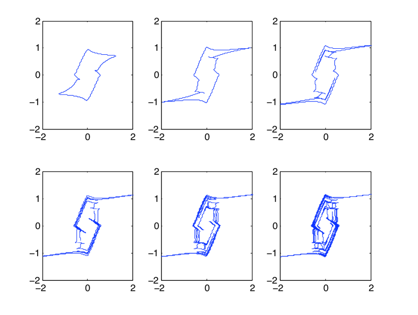
Figure 6: The image of under the first six iterates under $x\mapsto M\circ R_{1/||x||}(x)$ of the set $||x||=1$.

where $R$ and $||z||$ are as above, and where $M$ is a matrix of the form $M=\left(\begin{array}[]{cc}2&0\\ 0&0.5\end{array}\right)$. Note that $F$ is a homeomorphism which is non-smooth at $0$. The image of a ray through $0$ under the map $F$ is a spiral, see the middle diagram in Figure 5. There exist $r\in(0,1)$ so that $F$ can send a point in the annulus $A_{n}:=\{z\in{\mathbb{R}}^{2};r^{n+1}\leq||z||\leq r^{n}\}$ to annuli $A_{n-1},A_{n},A_{n+1}$ in a way which almost completely ‘forgets’ where the point started from. So the dynamics can be essentially modelled by that of a random walk. Indeed, it was proved in [22] that there are orbits which can go to $0$ at a prescribed speed. The image of a set $\{z\in{\mathbb{R}}^{2};||z||=1\}$ under the first six iterates of $F$ is drawn in Figure 6.

.....................................................................................................................................................................................................................................................................................................................................................................................................................................................................................................................................................................................................................................................................................................$Z$$D$$\Gamma$.........................................................................................................................................................................................................................................................................................................................................................................................................................................................................................................................................................................................................................................................................................................................................................................................................................................................................................................................................................................................................................................................................................................................................$l$.............................................................................................................................................................................................................................................................................................................................................................................................................................................................................................................................................................................................................................................................................................................................................................................................................................................................................................................................................................................................................................................................................................................................................................................................................................................................................................................................................................................................................................................................................................................................................................................................................................................................................................................................................................................................................................................................................................................................................................................................................................................................................................................................................................................................................................................................................................................................................................................................................................................................................................................................................................................................................................................................................................................................................................................................................................................................................................................................................................................................................................................................................................................................................................................................................................................................................................................................................................

Figure 5: On the left, the orbit $\Gamma$ with a transversal section $Z$. $\Gamma$ is a hexagon in ${\mathbb{R}}^{4}$, and is here presented as a genuine hexagon. In the middle, the image of a half-ray $l$ through $0$ under the model map $F$ defined in (7.25) is drawn. A conveniently chosen curve $l$ contains a sequence of fixed points, converging to $0$. On the right, a nested sequence of annuli $A_{n}$ in $Z$ is drawn. There exist orbits which visit annuli $A_{n(i)}$ where $n(i)$ can be chosen arbitrarily so that $|n(i+1)-n(i)|\leq 1$ and $n(i)\geq 0$.

7.3 The existence of a global section

In the example considered in the previous theorem, $H^{-1}$ is homeomorphic to $S^{3}$, i.e. to ${\mathbb{R}}^{3}\cup\{\infty\}$. It turns out that the flow has a global first return section $S$, namely a topological disc spanned by the periodic orbit $\Gamma$.

Theorem 7.2 (Existence of a global first return section through $\Gamma$).

For the Hamiltonian differential inclusion defined in Theorem 7.1, there exists a topological disc $S\subset H^{-1}(1)\approx S^{3}$ whose boundary is equal to the periodic orbit $\Gamma$ so that the following properties hold:

1. The orbit through each point $x\in H^{-1}(1)\setminus\Gamma$ intersects the topological disc $S$ infinitely many times (and each of these intersections is transversal). So $S$ is a global section with a well-defined first return map $R_{S}$.

2. The first return time of $z$ to $S$ tends to zero when $z\in S\setminus\Gamma$ tends to $z^{\prime}\in\Gamma$.

3. The first return map $R_{S}$ to $S$ has a continuous extension to $\partial S$ and $R_{S}|\partial S=id$.

4. One can choose $S$ to be the union of four (two-dimensional) triangles in ${\mathbb{R}}^{4}$ and so that $R_{S}$ is piecewise affine and area preserving.

5. $R_{S}$ has homoclinic intersections of periodic orbits, and hence horseshoes.

Of course, a smooth vector field could never have such a global section.

7.4 Visualising the dynamics in $S^{3}$.

The existence of the global section $S$ makes it rather easy to visualize the flow. The set $S$ is a union of four triangles in ${\mathbb{R}}^{4}$, and a projection of this set is drawn in Figure 7. As is shown in [22] the following holds.

1. The flow on $H^{-1}(1)\approx S^{3}={\mathbb{R}}^{3}\cup\{\infty\}$ has exactly one periodic orbit which meets the section $S$ once. This periodic orbit is of saddle-type.

2. The flow has exactly one periodic orbit $c$ which meets the section $S$ twice. This periodic orbit $c$ is elliptic and intersects $S$ in the centers of the two ‘egg-like’ regions shown in $S$. The ‘egg-like’ regions are filled by invariant circles (corresponding to invariant tori for the flow). This can be seen as follows: $c\cap D$ consists of two points $p_{1},p_{2}$. As mentioned, the first return map $R_{S}$ to $S$ is a piecewise affine map. Moreover, the linearisation of $R_{S}^{2}$ at $p_{1}$ has two complex conjugate eigenvalues on the unit circle (not equal to one), see [22]. It follows that $R_{S}^{2}$ is linearly conjugate to a rotation, and so orbits near $x_{0}$ lie on ellipses.

As mentioned, in the previous the previous theorem, $\Gamma$ is a periodic orbit of the flow on the boundary of $S$, and each other orbit of the flow in $H^{-1}(1)\approx S^{3}={\mathbb{R}}^{3}\cup\{\infty\}$ transversally intersects the section $S\setminus\Gamma$ infinitely many times.

7.5 Open problems

Many questions are still open about this specific system. For example, from the above description it follows that $H^{-1}(1)$ is the union of two fully invariant sets $\mathcal{U}$ and $\mathcal{W}$ where $\mathcal{U}$ consists of a closed solid torus which intersects $S$ in the two ‘egg-shaped’ regions and where $\mathcal{W}$ is the complement (so $\mathcal{W}$ is the interior of a solid torus).

Question 7.3.

Does there exist an orbit in $\mathcal{W}$ which is dense in $\mathcal{W}$?

If one considers the first return map to $S$ one can ask:

Question 7.4.

Consider the first return map $R_{s}\colon S\to S$.

1. Are there any other elliptic orbits (of higher period)?

2. Take a (Lebesgue typical) point $x\in\mathcal{W}$. What can be said about the limits of $\dfrac{1}{n}\sum_{i=0}^{n-1}\delta_{R^{i}(x)}$? Does it exist? Is it unique? Is it absolutely continuous?

3. Is it possible to find an adequate random-walk description of the first return map to a section $\Sigma$?

It would also be interesting to understand the dynamics of the map $F(x)=M\circ R_{1/||x||}(x)$ as in (7.25) more thoroughly, where $R_{\theta}(x)$ is a rotation and $M$ is a linear map of saddle-type. For example, are typical orbits dense in ${\mathbb{R}}^{2}$ for generic matrices $M$? For some results on this, see [22].

More general questions are posed in the conclusion, see Section 9.

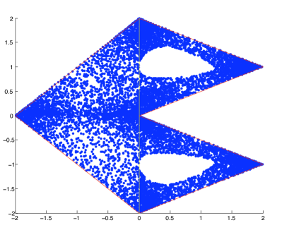
Figure 7: A projection of the global section $S$. Note that $S$ is topological disc whose boundary is a hexagon $\Gamma$ where $\Gamma$ is a periodic orbit of the flow. Orbits spiral around $\Gamma$ as in Figure 4. Note that we have drawn the hexagon differently than in Figure 5 (the reason for drawing $S$ in this way is that it represents better how $S$ is naturally embedded in $H^{-1}(1)=S^{3}$ as is explained in Section 3 of [22]). We also plot the orbit of a typical starting point under the first return map to $S$. There are two ’egg-shaped’ regions which are permuted by the first return map. Orbits within this region form invariant circles (these ’egg-shaped’ regions have period two). At the center of these regions there is a periodic orbit of period two. Locally, the map is a rigid rotation over an angle which is determined by the parameter $\beta$. For $\beta=\sigma$ the rotation angle is an irrational number, so orbits under the first return map lie on circles.

8 Application to zero sum games

In this section we will apply the previous results to to fictitious play and best response dynamics defined in game theory and state some applications of our results which are relevant to game theory.

Let us first give a short introduction into the relevant notions from game theory. Consider a two-player game where player $P$ has a choice of $m$ actions and player $Q$ has a choice of $n$ actions for each time $t\in[1,\infty)$. So let $\Sigma_{p}\subset{\mathbb{R}}^{m}$ and $\Sigma_{q}\subset{\mathbb{R}}^{n}$ be the space of probability vectors in ${\mathbb{R}}^{m}$ resp. ${\mathbb{R}}^{n}$. For each $t\in[0,\infty)$, each of the players continuously chooses an action

$$m^{P}(t)\in\{e_{1}^{p},\dots,e_{m}^{p}\}\subset\Sigma_{p}\mbox{ and }m^{Q}(t)\in\{e_{1}^{q},\dots,e_{n}^{q}\}\subset\Sigma_{q}.$$

Let

$$p(t)=\dfrac{1}{t}\int_{s=1}^{t}m^{P}(s)\,ds\mbox{ and }q(t)=\dfrac{1}{t}\int_{s=1}^{t}m^{Q}(s)\,ds.$$ (8.26)

Hence $p(t)\in\Sigma_{p}$ describes the average of the strategies player $P$ has chosen during the time interval $[1,t)$. Usually $p(t)$ and $q(t)$ are called the strategy profiles of players $P$ and $Q$.

In this model, it assumed that player $P$ only observes (or responds to) $q(t)$ and tries to choose an action which maximizes his payoff. In other words, it is assumed that there are best-response maps (possibly multivalued) $\Sigma_{q}\ni q\mapsto{\mathcal{B}\!\mathcal{R}\!}_{p}(q)\in\Sigma_{p}$ and $\Sigma_{p}\ni p\mapsto{\mathcal{B}\!\mathcal{R}\!}_{p}(p)\in\Sigma_{q}$. One often makes the assumption that there are $n\times m$ matrices $P,Q$ so that

$${\mathcal{B}\!\mathcal{R}\!}_{p}(q):=\operatorname*{arg\,max}_{p\in\Sigma_{p}}p^{\prime}\,Pq\mbox{ and }{\mathcal{B}\!\mathcal{R}\!}_{q}(p):=\operatorname*{arg\,max}_{q\in\Sigma_{q}}p^{\prime}\,Qq.$$

It is then assumed that player $P$ chooses at time $t$ an action $m^{P}(t)$ for which

$$m^{P}(t)\in{\mathcal{B}\!\mathcal{R}\!}_{p}(q(t))$$ (8.27)

while $Q$ chooses an action

$$m^{Q}(t)\in{\mathcal{B}\!\mathcal{R}\!}_{q}(p(t)).$$ (8.28)

Differentiating (8.26) immediately leads to

$$\dfrac{dp}{dt}=\dfrac{1}{t}(m^{P}(t)\,-p(t)),\quad\dfrac{dq}{dt}\in\dfrac{1}{t}(m^{Q}(t)-q(t))$$ (8.29)

and combining this with (8.27) and (8.28) gives that $t\mapsto(p(t),q(t))$ is a solution to the following differential inclusion

$$\dfrac{dp}{dt}\in\dfrac{1}{t}({\mathcal{B}\!\mathcal{R}\!}_{p}(q)\,-p),\quad\dfrac{dq}{dt}\in\dfrac{1}{t}({\mathcal{B}\!\mathcal{R}\!}_{q}(p)-q).$$ (8.30)

This is called fictitious play dynamics. Some authors prefer a different time parametrization (taking $s=e^{t}$), which gives

$$\dfrac{dp}{ds}={\mathcal{B}\!\mathcal{R}\!}_{A}(q)\,-p,\dfrac{dq}{ds}={\mathcal{B}\!\mathcal{R}\!}_{B}(p)-q.$$ (8.31)

and this is called best response dynamics. As noted before, it is not hard to show that these differential inclusions have solutions, see [2]). Best response dynamics is commonly associated with two infinite populations, so that within each of these two populations the fraction of players choosing a certain strategy continuously evolves towards best response, see [13]. A common interpretation of fictitious play is as a model for rational learning, see for example Fudenberg and Levine [7].

In the present paper we consider the zero-sum case. In this situation, the players have opposite interests and so we have $P=\,{\mathcal{M}}\,$ and $Q=-\,{\mathcal{M}}\,$.

A more detailed explanation of the rationale of this model can be found in for example the monograph of Fudenberg and Levine [7]. One reason this model is used widely is because it is frequently used as a learning model in economic theory.

Restating our previous results gives:

Theorem 8.1.

Assume that we have a $m\times n$ two-player zero-sum game with $m$ and $n$ not necessarily equal. Assume that the transversality condition (2.8) holds. Then

1. the Nash equilibrium $({\bar{p}},{\bar{q}})$ is unique;

2. (8.31) and (8.30) define continuous flows converging to the Nash equilibrium $({\bar{p}},{\bar{q}})$;

3. there exist $r\leq\min(m,n)$ and $i_{1},\dots,i_{r}\in\{1,\dots,m\}$ and $j_{1},\dots,j_{r}\in\{1,\dots,n\}$ so that ${\bar{p}}\in[e_{i_{1}},\dots,e_{i_{r}}]\subset\Sigma_{p}$ and ${\bar{q}}\in[e_{j_{1}},\dots,e_{j_{r}}]\subset\Sigma_{q}$ and so that moreover the $i_{1},\dots,i_{r}$-th component of ${\bar{p}}$ and $j_{1},\dots,j_{r}$-th component of ${\bar{q}}$ are non-zero (in other words, $({\bar{p}},{\bar{q}})$ is a completely mixed Nash equilibrium w.r.t. to this subgame);

4. points starting in $[e_{i_{1}},\dots,e_{i_{r}}]\times[e_{j_{1}},\dots,e_{j_{r}}]$ stay in this subspace under the flow;

5. the other components of $p,q$ decrease monotonically with time for any solution of the differential equations (8.31) and (8.30).

6. each half-line through $(\bar{p},\bar{q})$ has a unique intersection with $H^{-1}(1)$; if we consider the flow restricted to $[e_{i_{1}},\dots,e_{i_{r}}]\times[e_{j_{1}},\dots,e_{j_{r}}]$ and project this onto $H^{-1}(1)$ we obtain a Hamiltonian flow.

That solutions converge to the Nash equilibrium was already proved in the 1950’s by Robinson [18]. According to the previous theorem, generically there is precisely one Nash equilibrium and this is a completely mixed Nash equilibrium for some $r\times r$ subgame (which is an invariant subset of the dynamics).

In the trivial case of a $2\times 2$ zero-sum game, orbits spiral towards the Nash equilibrium. If we take $H$ as before, then we obtain an induced Hamiltonian flow on $H^{-1}(c)$, $c>0$. It turns out that $H^{-1}$ is the boundary of a quadrilateral and the Hamiltonian flow moves either clockwise or counter clockwise on this boundary, see Figure 8.

In the higher dimensional case of a $k\times k$ game with $k\geq 3$, typical orbits will be more complicated. Indeed, since a Hamiltonian flow preserves volume, it follows from the Poincaré recurrence theorem that Lebesgue almost every point returns to a neighbourhood of the initial point, see [23]. In the example we presented, for typical starting points, players switch strategies erratically.

The examples considered in Theorem 7.1 are relevant to a result of Krishna and Sjöström (see [11]). Their result deals with orbits with cyclic play. More precisely, one has cyclic play along the orbit $t\mapsto(p(t),q(t))$ if the values of $t\mapsto({\mathcal{B}\!\mathcal{R}\!}_{p}(q(t)),{\mathcal{B}\!\mathcal{R}\!}_{q}(p(t))$ are changing periodically with some period $s\in\{1,2,\dots,\}$, i.e., if there exists times $t_{0}<t_{1}<t_{2}<t_{3}<t_{4}<\dots$ so that for all $i\geq 0$ and all $t\in(t_{i},t_{i+1})$,   $({\mathcal{B}\!\mathcal{R}\!}_{p}(q(t)),{\mathcal{B}\!\mathcal{R}\!}_{q}(p(t))$ is equal to some corner point in $V_{i}\in\Sigma_{p}\times\Sigma_{q}$ and so that $V_{i+s}=V_{i}$ for all $i\geq 0$. In other words, both players repeat strategies every $s$-th step. The theorem of Krishna and Sjostrom states that for generic games, it is impossible for an open set of initial conditions to all converge to the Nash equilibrium with the same cyclic play. The next corollary shows that their theorem does NOT hold for non-generic games (in particular not for zero sum games):

Corollary 8.2.

There exists an open set of matrices, so that the corresponding zero-sum games have the following property: for an open set of initial conditions one has convergence to the Nash equilibrium with cyclic play.

Proof.

Consider the zero-sum game associated to the matrix (7.24) and take an orbit corresponding to an initial condition which lies in one of the two egg-shaped region in Figure 7. Here the region bounded by the six sides forms the global section $S$ from Theorem 7.2 associated to the flow induced on $H^{-1}(1)$ and the ‘centres’ of the two egg-shaped regions in Figure 7 correspond to a periodic two orbit $\gamma$ of the first return map to $S$. Let $D\cap\gamma=\{x_{0},x_{1}\}$ and let $F$ be the second iterate of the first return map to $S$. Then $F(x_{0})=x_{0}$ and it is shown in [21] and [22] that the linearisation of $F$ at $x_{0}$ has eigenvalues $\lambda,\bar{\lambda}$ with $|\lambda|=1$. This orbit corresponds to the Shapley orbit in [21] and [22] and as was shown there, the periodic orbit $\gamma$ crosses the indifference sets exactly 6 times (each time transversally). Now consider an orbit $\tilde{\gamma}$ near $\gamma$. Since the first return map $R_{S}$ to $S$ is a piecewise translation, near $x_{0}$ the second iterate $R_{s}^{2}$ is a (smooth) rotation. Here we use that $\gamma$ meets all indifference sets (sets where ${\mathcal{B}\!\mathcal{R}\!}_{p}$ or ${\mathcal{B}\!\mathcal{R}\!}_{q}$ are multivalued) transversally. It follows that $\tilde{\gamma}\cap D$ lies on two circles around $x_{0}$ resp. $x_{1}$ (provided $\tilde{\gamma}$ is sufficiently close to $\gamma$). It also follows that $\tilde{\gamma}$ hits all the indifference sets transversally and in the same order as $\gamma$. (But of course the times at which $\tilde{\gamma}$ hits the indifference planes need not necessarily be periodic.) In any case, all orbits $\tilde{\gamma}$ sufficiently near $\gamma$ have periodic play.

All this also holds for all zero-sum games near the one considered in Theorem 7.1. Indeed, the eigenvalues of the linearization of $R_{S}^{2}$ at $x_{0}$ both lie on the unit circle. Since these eigenvalues are not equal to one, they are complex conjugate. Hence for a nearby game the corresponding map $\tilde{R}_{S}^{2}$ also has a fixed point at a point $\tilde{x}_{0}$ close to $x_{0}$, and the linearization of $\tilde{R}_{S}^{2}$ at $\tilde{x}_{0}$ also has two eigenvalues which are complex conjugate. Since $\tilde{R}_{S}^{2}$ is area preserving, the two eigenvalues again lie on the unit circle. ∎

....................$\bullet$$\bullet$$\bullet$$\bullet$..............................................................................................................................................................................................................................................................................................................................................................................................................................................................................................................................................................................................................................................

Figure 8: A $2\times 2$ zero-sum game converges to the Nash equilibrium. The level set $H^{-1}(c)$ is a quadrilateral and the Hamiltonian flow moves periodically on this.

8.1 Non-zero sum games

Even in the case when the players are involved in a general sum game, the above differential inclusion (8.31) makes sense. There are many papers which show that one has convergence to the equilibrium in particular situations: for games where one or both of the players have only 2 strategies to choose from, see [15] and [14] for the $2\times 2$ case; [19] for the $2\times 3$ case; and [3] for the general $2\times n$ case. A $2\times 2\times 2$ fictitious game with a stable limit cycle was constructed in [10]. The $3\times 3$ example studied in this paper, shows that the situation is far more complicated in general, see [21] and [22]. Theorem 7.1 summarises some of the results from these last two papers.

9 Conclusion

In this paper we saw that the Hamiltonian function $H$ defined as in (2.3) generates a Hamiltonian vector field (which is piecewise constant) with a continuous translation flow. We also described an example, showing that the dynamics of such systems can be surprisingly rich. Even though many questions remain about the case considered, it may be a good idea to consider more elementary questions in general. For example, the following question is very natural, and seems wide open.

Question 9.1.

Assume that $H$ is as in (2.3) where $\,{\mathcal{M}}\,$ satisfies all the transversality conditions.

1. Does the flow necessarily have periodic orbits?

2. Are there always infinitely many periodic orbits?

3. Can the set of periods of periodic orbits be discrete?

4. Are orbits dense in certain open sets?

In the vain of the Palis conjecture, see [17], one can also ask questions about the statistical behaviour of orbits:

Question 9.2 (A version of the Palis conjecture).

Assume that $H$ is as in (2.3) where $\,{\mathcal{M}}\,$ satisfies all the transversality conditions.

1. Can these systems be ever structurally stable (within the class of systems under consideration)?

2. What are the possible physical measures for these systems?

References

- [1] V. I. Arnol’d. Instability of dynamical systems with many degrees of freedom. Dokl. Akad. Nauk SSSR, 156:9–12, 1964.
- [2] Jean-Pierre Aubin and Arrigo Cellina. Differential inclusions, volume 264 of Grundlehren der Mathematischen Wissenschaften [Fundamental Principles of Mathematical Sciences]. Springer-Verlag, Berlin, 1984. Set-valued maps and viability theory.
- [3] Ulrich Berger. Fictitious play in games. J. Econom. Theory, 120(2):139–154, 2005.
- [4] G. W. Brown. Some notes on computation of games solutions’. The Rand Corporation, P-78, April., 1949.
- [5] George W. Brown. Iterative solution of games by fictitious play. In Activity Analysis of Production and Allocation, Cowles Commission Monograph No. 13, pages 374–376. John Wiley & Sons Inc., New York, N. Y., 1951.
- [6] Mario di Bernardo, Chris J. Budd, Alan R. Champneys, Piotr Kowalczyk, Arne B. Nordmark, Gerard Olivar Tost, and Petri T. Piiroinen. Bifurcations in nonsmooth dynamical systems. SIAM Rev., 50(4):629–701, 2008.
- [7] Drew Fudenberg and David K. Levine. The theory of learning in games, volume 2 of MIT Press Series on Economic Learning and Social Evolution. MIT Press, Cambridge, MA, 1998.
- [8] Christopher Harris. On the rate of convergence of continuous-time fictitious play. Games Econom. Behav., 22(2):238–259, 1998.
- [9] J. Hofbauer. Stability for the best response dynamics. Preprint, University of Vienna, 1995.
- [10] J. S. Jordan. Three problems in learning mixed-strategy Nash equilibria. Games Econom. Behav., 5(3):368–386, 1993.
- [11] Vijay Krishna and Tomas Sjöström. On the convergence of fictitious play. Math. Oper. Res., 23(2):479–511, 1998.
- [12] Markus Kunze. Non-smooth dynamical systems, volume 1744 of Lecture Notes in Mathematics. Springer-Verlag, Berlin, 2000.
- [13] Akihiko Matsui. Best response dynamics and socially stable strategies. J. Econom. Theory, 57(2):343–362, 1992.
- [14] Andrew Metrick and Ben Polak. Fictitious play in games: a geometric proof of convergence. Econom. Theory, 4(6):923–933, 1994. Bounded rationality and learning.
- [15] K. Miyasawa. On the convergence of the learning process in a non-zero-sum two-person game. Economic Research Program, Princeton University, Research Memorandum No. 33., 1961.
- [16] Martin J. Osborne and Ariel Rubinstein. A course in game theory. MIT Press, Cambridge, MA, 1994.
- [17] J. Palis. Open questions leading to a global perspective in dynamics. Nonlinearity, 21(4):T37–T43, 2008.
- [18] Julia Robinson. An iterative method of solving a game. Ann. of Math. (2), 54:296–301, 1951.
- [19] Aner Sela. Fictitious play in games. Games Econom. Behav., 31(1):152–162, 2000.
- [20] L. S. Shapley. Some topics in two-person games. In Advances in Game Theory, pages 1–28. Princeton Univ. Press, Princeton, N.J., 1964.
- [21] Colin Sparrow, Sebastian van Strien, and Christopher Harris. Fictitious play in games: the transition between periodic and chaotic behaviour. Games Econom. Behav., 63(1):259–291, 2008.
- [22] Sebastian van Strien and Colin Sparrow. Fictitious play in games: chaos and dithering behaviour”. Accepted for publication in Games and Econom. Behav. Preprint 2009 http://arxiv.org/abs/0903.4847.
- [23] Peter Walters. An introduction to ergodic theory, volume 79 of Graduate Texts in Mathematics. Springer-Verlag, New York, 1982.