Combined Modeling of Acceleration, Transport, and Hydrodynamic Response in Solar Flares: I. The Numerical Model

Abstract

Acceleration and transport of high-energy particles and fluid dynamics of atmospheric plasma are interrelated aspects of solar flares, but for convenience and simplicity they were artificially separated in the past. We present here self-consistently combined Fokker-Planck modeling of particles and hydrodynamic simulation of flare plasma. Energetic electrons are modeled with the Stanford unified code of acceleration, transport, and radiation, while plasma is modeled with the Naval Research Laboratory flux tube code. We calculated the collisional heating rate directly from the particle transport code, which is more accurate than those in previous studies based on approximate analytical solutions. We repeated the simulation of Mariska et al. (1989) with an injection of power-law, downward beamed electrons using the new heating rate. For this case, a $\sim$10% difference was found from their old result. We also used a realistic spectrum of injected electrons provided by the stochastic acceleration model, which has a smooth transition from a quasi-thermal background at low energies to a nonthermal tail at high energies. The inclusion of low-energy electrons results in relatively more heating in the corona (vs. chromosphere) and thus a larger downward heat conduction flux. The interplay of electron heating, conduction, and radiative loss leads to stronger chromospheric evaporation than obtained in previous studies, which had a deficit in low-energy electrons due to an arbitrarily assumed low-energy cutoff. The energy and spatial distributions of energetic electrons and bremsstrahlung photons bear signatures of the changing density distribution caused by chromospheric evaporation. In particular, the density jump at the evaporation front gives rise to enhanced emission, which, in principle, can be imaged by X-ray telescopes. This model can be applied to investigate a variety of high-energy processes in solar, space, and astrophysical plasmas.

1. Introduction

A solar flare, as one of the most prominent manifestations of solar activity, has many faces among which are acceleration and transport of high-energy particles and the dynamical response of atmospheric plasma. It is generally believed that magnetic reconnection in the corona is the primary energy release mechanism that leads to plasma heating and particle acceleration. The heated plasma and accelerated particles (primarily electrons) produce bremsstrahlung X-rays at the apex of the flare loop observed as a loop-top (LT) source (e.g., Masuda et al., 1994; Petrosian et al., 2002; Krucker & Lin, 2008). Some of the released energy is transported down the closed magnetic loop by nonthermal particles (electrons and ions) and thermal conduction, which contribute to energy gain in various layers of the atmosphere. Electrons give up most of their energy to ambient particles via Coulomb collisions, and produce hard X-rays (HXRs) primarily at the footpoints (FPs) of the loop in the dense transition region (TR) and chromosphere (see Hoyng, 1981; Sakao, 1994; Saint-Hilaire et al., 2008). Accelerated protons and heavier ions, on the other hand, cause nuclear reactions while colliding with background particles and produce $\gamma$-rays. Some accelerated electrons and ions escape along open magnetic field lines into the interplanetary space and are observed as solar energetic particles (SEPs) by in situ instruments (e.g., Lin, 1985; Liu et al., 2004a; Krucker et al., 2007). The rate of energy gain in the chromosphere, if exceeding the combined local radiative and conductive cooling rate, can rapidly heat the plasma up to a temperature of $\sim$$10^{7}$ K. The resulting overpressure drives an upward mass flow at a speed up to hundreds of km s^-1, which fills the flare loop with a hot plasma, giving rise to the gradual increase of soft X-ray (SXR) emission. This process, termed chromospheric evaporation by Neupert (1968), can influence particle transport by changing the ambient density in the loop on timescales of tens of seconds, and affect heat conduction by changing the loop temperature distribution at the same time. Collisional and conductive heating will be consequently modified, and in turn, so will the dynamic atmospheric response. On longer timescales of minutes, as magnetic reconnection proceeds and new loops are formed or excited, the above processes repeat sequentially in newer loops.

1.1. Motivation for This Study

The aforementioned processes are coupled in a circular chain, but due to great complexity of the subject, previous researchers tended to focus on one process at a time while assuming some simple forms for others. Past investigations fall into two general categories: (1) acceleration and transport of particles and (2) fluid dynamics of atmospheric plasma.

(1) Various mechanisms have been proposed for particle acceleration. Among the agents of acceleration are DC electric fields (Holman, 1985; Litvinenko, 1996; Zharkova & Gordovskyy, 2004), shocks (Tsuneta & Naito, 1998), and turbulence or plasma waves (Ramaty, 1979; Hamilton & Petrosian, 1992; Miller et al., 1996; Petrosian & Liu, 2004). Particle transport is comparatively better understood and previous studies usually assumed a hydrostatic atmosphere. Early analytical studies (Brown, 1973; Petrosian, 1973; Lin & Hudson, 1976; Emslie, 1978; Chandrashekar & Emslie, 1987) took various approximations (e.g., neglecting pitch-angle diffusion) to allow the problem to be tractable. The numerical study of Leach & Petrosian (1981) improved on this by solving the Fokker-Planck transport equation with inclusion of pitch-angle changes due to Coulomb collision and magnetic mirroring. This was later extended to the relativistic regime by including energy losses and pitch-angle changes due to synchrotron radiation (McTiernan & Petrosian, 1990). Similar Fokker-Planck studies of particle transport were performed by MacKinnon & Craig (1991), McClements (1992), and Syniavskii & Zharkova (1994).

(2) Fluid dynamics of the magnetized atmosphere in response to flare heating can be best studied with a multi-dimensional magnetohydrodynamic (MHD) model, but for simplicity most efforts were invested in one-dimensional hydrodynamic (HD) simulations. This is justified for the solar corona where the magnetic pressure dominates the gas pressure (low $\beta$ plasma) and resistivity is low. As a result, plasma is only allowed to flow along the magnetic field lines due to the line-tying condition. Previous HD models (MacNeice et al., 1984; Nagai & Emslie, 1984; Emslie & Nagai, 1985; Fisher et al., 1985a, b, c; Mariska et al., 1989; Gan & Fang, 1990; Emslie et al., 1992) usually assumed a power-law spectrum of accelerated electrons injected at the apex of the loop, and calculated collisional heating along the loop by these electrons from approximate analytical solutions of particle transport mentioned above. Abbett & Hawley (1999) and Allred et al. (2005) improved on previous studies by including detailed calculation of radiative transfer in the atmosphere.

There are theoretical and observational motivations to investigate the particle and fluid aspects of a solar flare together in a self-consistent manner. From a theoretical point of view, such an investigation is demanded in order to retrieve missing physics when the two aspects were studied separately. It has also become technically more feasible, thanks to advances in both aspects over the last three decades and particularly in recent years. Several studies (Miller & Mariska, 2005; Winter et al., 2007) along this direction are already under way, but none of them has been completed. From an observational point of view, new observations, particularly X-ray images and spectra obtained by the current Ramaty High Energy Solar Spectroscopic Imager (RHESSI) and previous Yohkoh missions, have posed new challenges to the existing theories. For example, in recent studies of the Neupert (1968) effect, Veronig et al. (2005) and Liu et al. (2006b) found that, unexpectedly, the electron energy deposition power, which is more physically related to the thermal energy change rate, did not yield a better correlation with the time derivative of the SXR flux than the conventional HXR flux. In an event of chromospheric evaporation imaged by RHESSI for the first time, Liu et al. (2006b) found X-ray sources moving from the FPs to the LT at very high speeds ($\sim$10³ km s^-1). More interestingly, Sui et al. (2006) found double nonthermal sources moving first downward from the LT toward the FPs and then upward along the loop. To fully understand these observations requires a joint study of acceleration and transport of particles and fluid dynamics of the atmospheric response.

1.2. Approach of This Study

With the goal to investigate the coupled processes of acceleration, transport, and hydrodynamics in solar flares, we present here combined Fokker-Planck modeling of particles and HD simulation of plasma. (1) The Fokker-Planck model utilizes the Stanford unified code of particle acceleration, transport, and bremsstrahlung radiation (Petrosian et al., 2001). The transport and radiation calculation is based on the work of Leach & Petrosian (1981, 1983) and McTiernan & Petrosian (1990). The acceleration module of the code adopts the stochastic acceleration model of Petrosian & Liu (2004, hereafter PL04), which has inherited knowledge accumulated over a decade (Hamilton & Petrosian, 1992; Dung & Petrosian, 1994; Park & Petrosian, 1995, 1996; Park et al., 1997). When compared with observations, this model has many attractive features and advantages (Liu et al., 2004a, 2006a, 2008) over other mechanisms. (2) The HD simulation uses the Naval Research Laboratory (NRL) Solar Flux Tube Model (Mariska, Emslie, & Li, 1989, hereafter MEL89), which, as a modified version of the Mariska et al. (1982) model, provides excellent treatment of fluid dynamics and has been widely used in studying atmospheric response to flare heating (e.g., Warren & Doschek, 2005).

One of the major advances marked by this study is the more accurate and self-consistent evaluation of the collisional heating rate by nonthermal electrons. This heating rate is critical to HD simulation of flares, but was not properly calculated previously in two major aspects: (1) The calculation of energy loss of energetic electrons and thus the heating rate was based on approximate analytical solutions (e.g., Brown, 1973; Emslie, 1978), which incorporated only pitch angle growth due to Coulomb collisions, but in reality the pitch angle change is a diffusion process. This will be remedied in this study with the inclusion of a full Fokker-Planck treatment of electron transport. (2) Another previous drawback was the use of an unrealistic spectrum of injected electrons, which usually was a power-law with a low-energy cutoff. Fisher et al. (1985c), for example, assumed a sharp low-energy cutoff at $E_{\rm c}=20\mathrm{\,keV}$ (i.e., no electrons below $E_{\rm c}$), while MEL89 introduced a “soft” cutoff below which the spectrum is still a power-law with a positive slope. It should be noted that rather than an intrinsic property of the primary accelerated electron population, a low-energy cutoff or turnover in the electron spectrum inferred from X-ray observations can result from secondary effects such as return currents (Zharkova & Gordovskyy, 2006) and photospheric albedo (Langer & Petrosian, 1977; Bai & Ramaty, 1978; Sui et al., 2007). The collisional heating rate is sensitive to the injected electron spectrum and thus the use of an incorrect spectrum would make the HD simulation deviate from reality significantly. PL04 has provided a more realistic electron spectrum that has a continuous span from a quasi-thermal distribution at low energies to a nonthermal tail at high energies, avoiding unnecessary low-energy cutoff. It also gives good fits to both LT and FP X-ray spectra obtained by RHESSI. Such an electron spectrum is used in this work. As we will see later, the low-energy electrons, which otherwise would have been missing if a cutoff were to be present, play an important role in heating and in influencing the subsequent HD evolution.

We present the numerical model in § 2, techniques to combine different modules of the model in § 3, and simulation runs in § 4. We compare the HD characteristics of different simulations in § 5 and examine the HD effects on particle transport and X-ray emission in § 6. Conclusions and discussions are given in § 7. This model is based on the PhD thesis of Liu (2006), which has also appeared as a book (Liu, 2008). The model has been refined ever since and the numerical results presented here are new. Our new calculations and analyses include: (1) recomputing the MEL89 simulation using our transport code (see §4.2), (2) detailed analysis of the interplay of heating and cooling (§5.2), and (3) examining the temperature distribution of plasma velocity which can be directly compared with Doppler observations (§5.3). In order to achieve more accuracy, we have extended the number of pitch angle bins from 24 to 100.

2. Simulation Model

Here we consider the dynamical evolution of a single flare loop perpendicular to the solar surface. As shown in Figure 1 (top), an acceleration region of length $L=5\mathrm{\,Mm}$ is located at the top of the model loop, sandwiched between two symmetric quarter-circles called the transport region of length $s_{\rm max}=14\mathrm{\,Mm}$. The loop has a uniform circular cross-section $a(s)=a_{0}=\pi r^{2}$ with a constant radius of $r=0.3\mathrm{\,Mm}$ at any distance $s$ from the edge of the acceleration region. In its initial state (Fig. 1, bottom) the loop spans from the hot ($T\gtrsim 10^{6}\mathrm{\,K}$), tenuous corona to the cold ($T=10^{4}\mathrm{\,K}$), dense chromosphere, with the TR (defined here as the lowest point where $T\geq 10^{5}\mathrm{\,K}$) located at $s_{\rm tr}\simeq 10\mathrm{\,Mm}$.

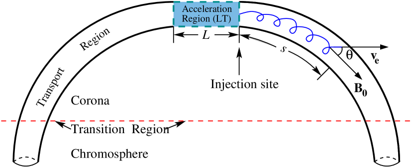
Figure 1.— Top: Geometry of the model flare loop. $\theta$ is the pitch angle of the electron with a velocity ${\bf v_{e}}$ in the guiding magnetic field ${\bf B_{0}}$. Bottom: Initial distribution of logarithmic temperature $T$, gas pressure $P$ (left scale), and electron number density $n_{e}$ (right scale) vs. distance in the transport region of the loop. Pressure is scaled upward by a factor of 100.

The simulation model includes four parts: (1) The stochastic acceleration code generates a spatially averaged distribution (in energy) of high-energy electrons in the acceleration region. This distribution is fed to the transport region where (2) the transport code computes the electron distribution (in energy and pitch angle) and collisional heating rate as a function of distance (depth), and (3) the hydrodynamic code simulates the atmospheric response to this heating. Finally, (4) the radiation code calculates the corresponding bremsstrahlung emission in the loop. Parts (1), (2), and (4) are inherited from the Stanford unified particle code (Petrosian et al., 2001) in which the acceleration module has been revised according to PL04, while part (3) is adopted from the NRL flux tube code (MEL89). Details of the four parts are described in the following subsections.

Note that sequential energizing (or excitation) propagating from one flare loop to another has been observed as the apparent motions of HXR LT (Gallagher et al., 2002; Sui & Holman, 2003) and FP (Grigis & Benz, 2005; Yang et al., 2009; Liu et al., 2009) sources. In our simulations, we set the duration of the impulsive phase to be 60 s. This time, according to Schrijver et al. (2006), translates into an apparent FP speed of ${2r\over 60\mathrm{\,s}}=10\mathrm{\,km}\mathrm{\,s}^{-1}$ (where $r=0.3\mathrm{\,Mm}$), which is comparable to the observed values (Liu et al., 2004b). Our single loop scenario is thus legitimate within the relevant timescale and can be viewed as an elementary process of sequential excitation of multiple loops. Evolution on longer timescales (say, $\gtrsim$100 s) involves multiple loops and can be studied by superimposing sequential single-loop simulations (e.g., Warren, 2006).

2.1. Stochastic Acceleration

The stochastic acceleration model of PL04 addresses electron and proton acceleration by plasma waves propagating parallel to the background magnetic field ${\bf B}_{0}$. According to this model, large-scale turbulence or long-wavelength plasma waves are generated in the corona as a result of magnetic reconnection. The turbulence, cascading to smaller scales, heats plasma and accelerates particles in a region near the top of the flaring loop. The heated plasma and accelerated electrons produce the observed thermal and nonthermal X-rays, respectively, in the acceleration region or the LT source (Xu et al., 2008; Liu et al., 2008). Here we briefly repeat the mathematical description of the model. The Fokker-Planck equation that governs electron acceleration, in general, can be written as

$${\partial f_{\rm ac}\over\partial t} = {\partial\over\partial E}\left[D(E){\partial f_{\rm ac}\over\partial E}\right]+{\partial\over\partial E}\{[A(E)-{\dot{E}}_{L}]f_{\rm ac}\}$$ (1)

$$-{f_{\rm ac}\over T_{\rm esc}(E)}+\dot{Q}(E)\,,$$

where $f_{\rm ac}\equiv f_{\rm ac}(t,E)$, in units of electrons $\mathrm{\,cm}^{-3}\mathrm{\,keV}^{-1}$, is the angle-integrated and spatially averaged electron distribution function in energy space (subscript “ac” denotes the acceleration region), $E$ is the electron kinetic energy, $D(E)$ is the energy diffusion coefficient, $A(E)$ the direct acceleration rate, $T_{\rm esc}(E)$ the particle escape time, $\dot{Q}(E)$ is the rate of background electrons being supplied to the acceleration region that serves as a source term, and finally ${\dot{E}}_{L}={\dot{E}}_{\rm Coul}+{\dot{E}}_{\rm synch}$ is the absolute value of the net energy loss rate that is a sum of the Coulomb and synchrotron loss rates.

In order to solve equation (1) one must first evaluate all the terms. The energy loss rates ${\dot{E}}_{\rm Coul}$ and ${\dot{E}}_{\rm synch}$ are well known (see eq. [18] of PL04) and the source term $\dot{Q}(E)$ is to be prescribed with a specific model (assumed to be a thermal or Maxwellian distribution here). The central task is then to obtain $D(E)$, $A(E)$, and $T_{\rm esc}(E)$. They are determined through the dispersion relation of the plasma waves (PL04 eq. [28]) and the wave-particle resonance condition (PL04 eq. [4]). Following PL04, we assume a fully ionized H and ⁴He plasma with a relative abundance of electron/proton/$\alpha$-particle=1/0.84/0.08, and a broken power-law spectrum of the turbulence given by equation (29) in PL04 with the relevant spectral indices $q_{l}=2$, $q=-1.7$ (Kolmogorov value), and $q_{h}=-4$. The characteristic acceleration rate $\tau_{p}^{-1}$ given by equation (30) in PL04 represents the rate of wave-particle interaction and depends on the level of turbulence.

Once all the coefficients have been evaluated, equation (1) is solved numerically using the flux conservative finite difference scheme of Chang & Cooper (1970) described in Park & Petrosian (1996). Here we assume a homogeneous acceleration region and obtain a steady state solution of $f_{\rm ac}(E)$ (i.e., $\partial/\partial t=0$). The angle-integrated flux in the acceleration region is $F_{\rm ac}(E)=v_{e}f_{\rm ac}(E)$, where $v_{e}$ is the electron velocity. We then calculate the flux of electrons that escape the acceleration region and enter the transport region of the flare loop,

$$F_{\rm esc}(E)={f_{\rm ac}(E)\over T_{\rm esc}(E)}L\,.$$ (2)

2.2. Particle Transport

The flux $F_{\rm esc}(E)$ is then input to the particle transport code (Leach & Petrosian, 1981; McTiernan & Petrosian, 1990) which calculates the electron distribution in energy and pitch-angle space and its variation with distance while the electrons spiral down magnetic field lines into deeper layers of the atmosphere. The code numerically solves the fully relativistic, steady-state, Fokker-Planck equation (i.e., eq. [1] in McTiernan & Petrosian 1990), which is similar to equation (1) here and includes energy loss (no energy diffusion) and pitch angle diffusion due to Coulomb collision, and pitch angle changes due to magnetic mirroring and synchrotron radiation. Following McTiernan (1989), we neglect return currents (Syniavskii & Zharkova, 1994; Zharkova et al., 1995).

The variable to be solved in the transport equation is the electron flux spectrum $F(E,\mu,s)$ as a function of energy $E$, cosine $\mu=\cos\theta$ of pitch angle $\theta$, and distance $s$ from the injection site at the boundary of the acceleration region. $F(E,\mu,s)d\mu$ has units of electrons $\mathrm{\,s}^{-1}\,\mathrm{\,cm}^{-2}\,\mathrm{\,keV}^{-1}$ and is evaluated as

$$F(E,\mu,s)=v_{e}f(E,\mu,s){a(s)\over a_{0}}\,,$$ (3)

where $f(E,\mu,s)d\mu$ is the number density distribution function in units of electrons $\mathrm{\,cm}^{-3}\,\mathrm{\,keV}^{-1}$ (cf., the angle-integrated number density $f_{\rm ac}(E)$ in the above acceleration code), and we integrate the differential electron flux $v_{e}f(E,\mu,s)$ over the cross-sectional area $a(s)$ of the loop and then normalize it by a constant equivalent area $a_{0}$. As noted earlier, here we assume a constant $a(s)=a_{0}$ for simplicity, which means a uniform magnetic field along the loop and thus no magnetic mirroring.

In addition to the injected electron flux $F_{\rm esc}(E)$ from the acceleration code, the transport code requires the knowledge of the ambient density and abundance distribution along the loop. (1) Here we assume that $F_{\rm esc}$ is isotropic in pitch angle, representing the consequence of frequent scatterings of electrons by turbulence in the acceleration region. This assumption is consistent with the nearly isotropic, rather than beamed, distributions inferred from center-to-limb variations of HXR and $\gamma$-ray fluxes and spectral indices in observations obtained by the Solar Maximum Mission (McTiernan & Petrosian, 1991), and more recently from atmospheric albedo due to Compton back-scattering in RHESSI flares (Kontar & Brown, 2006; Kašparová et al., 2007). The injected flux at the top ($s=0$) of each leg of the loop is then $F(E,\mu,s)|_{s=0}=F_{\rm esc}(E)/\int_{-1}^{1}d\mu$ which is equivalent to a uniform distribution in the $4\pi$ solid angle integrated over the $2\pi$ range of the azimuthal angle $\phi$ assuming axis-symmetry. With the symmetric assumption, the steady state calculation is performed in only one leg of the loop. We impose a symmetric (or reflective) boundary condition at $s=0$, where a particle leaving the computational domain is reflected back with identical energy but opposite pitch angle cosine, mimicking a particle coming from the other leg of the loop. (2) As to the background atmosphere, we assume a fully ionized hydrogen plasma whose distribution is taken from the result of the HD code described next.

2.3. Hydrodynamics

Hydrodynamics in the transport region is calculated with the NRL solar flux tube code (MEL89) based on Mariska et al. (1982). The code assumes a two-fluid plasma composed of electrons and ions that can only move along the magnetic field in a flux tube. The user-specified geometry of the tube (a uniform quarter-circle in our case) is characterized by the tube cross-sectional area $a(s)$ and the component of the gravitational acceleration along the tube. The code solves the time-dependent, one-dimensional equations of mass, momentum, and energy conservation (see eqs.[1]–[3] in MEL89). The independent variables are the mass density $\rho(s)$, fluid velocity $v(s)$, and temperature $T(s)$ which we assume to be the same for electrons and ions. Because of small masses of electrons, we neglect the momentum loss of energetic electrons to the background plasma.

The volumetric heating rate in the energy equation is

$$S(s)=S_{e}(s)+S_{0}\,,$$ (4)

where $S_{e}(s)$ represents heating by energetic electrons, which is provided by the transport code (see §3), and $S_{0}=8.31\times 10^{-3}\mathrm{\,ergs}\mathrm{\,s}^{-1}\mathrm{\,cm}^{-3}$ (MEL89) represents uniform background heating, presumably caused by coronal heating in the quiet sun active region. The conductive flux $F_{\rm cond}$ and heating rate $S_{\rm cond}$ are

$$F_{\rm cond}=-\kappa\frac{\partial T}{\partial s},\,\,\,\,\,\,S_{\rm cond}=-\frac{\partial F_{\rm cond}}{\partial s}\,,$$ (5)

where $\kappa$ is the thermal conductivity. The radiative energy loss rate is

$$L_{\rm rad}=n_{e}n_{p}\Phi(T)\,,$$ (6)

where $n_{e}$ and $n_{p}$ are the electron and proton number density, respectively, which are equal by our assumption of fully ionized hydrogen plasma, and $\Phi(T)$ is the optically-thin radiative loss function (MEL89) which has its maximum at $T\simeq 1-3\times 10^{5}\mathrm{\,K}$.

We select an adaptive mesh of 450 grids that move with time to optimize spatial resolution in the dense chromosphere and near sharp jumps at the TR and evaporation front. This mesh is also shared by the transport and bremsstrahlung radiation codes in our new model. A reflective (or symmetric) boundary condition is imposed at both the upper (loop apex) and lower (deep in the chromosphere) boundaries of the transport region (see Fig. 1), such that the system remains closed.

2.4. Bremsstrahlung Radiation

Having obtained the electron flux from the transport code and the background density from the HD code, we calculate the thin-target bremsstrahlung radiation intensity or photon emission rate, $I(\epsilon,s)$, as a function of photon energy $\epsilon$ and distance $s$. $I(\epsilon,s)$ (photons $\mathrm{\,s}^{-1}\,\mathrm{\,cm}^{-3}\,\mathrm{\,keV}^{-1}$) is defined as

$$I(\epsilon,s)=\int_{\epsilon}^{\infty}dE\left[n_{p}(s){d\sigma(\epsilon,E)\over d\epsilon}\right]F_{\rm int}\,,$$ (7)

where $d\sigma(\epsilon,E)/d\epsilon$ is the angle-averaged differential bremsstrahlung cross-section given by Koch & Motz (1959), and $F_{\rm int}=\int_{-1}^{1}F(E,s,\mu)d\mu$ is the angle-integrated electron flux. Substituting $F_{\rm int}$ with the acceleration region flux $F_{\rm ac}$ gives the LT emission $I_{\rm LT}(\epsilon)$, while identifying $F_{\rm int}=LF_{\rm thick}$ yields the spatially integrated thick-target emission $I_{\rm thick}(\epsilon)$ (Brown, 1971; Petrosian, 1973). Here $F_{\rm thick}=v_{e}f_{\rm thick}$ is the equivalent thick-target electron flux, given by the corresponding number density (Petrosian & Donaghy 1999; PL04)

$$f_{\rm thick}(E)={1\over L\dot{E}_{L}}\int_{E}^{\infty}F_{\rm esc}(E^{\prime})dE^{\prime}\,.$$ (8)

The equivalent FP emission is the spatially averaged photons emitted below the TR (located at $s_{\rm tr}$), $I_{\rm FP}(\epsilon)=\int_{s_{\rm tr}}^{s_{\rm max}}I(\epsilon,s)ds/(s_{\rm max}-s_{\rm tr})$, where $s_{\rm max}$ is the distance at the lower boundary of the loop. If the coronal is negligibly tenuous and the column depth at $s_{\rm max}$ is large enough to stop all HXR producing electrons of interest, $(s_{\rm max}-s_{\rm tr})I_{\rm FP}(\epsilon)$ approaches $I_{\rm thick}(\epsilon)$.

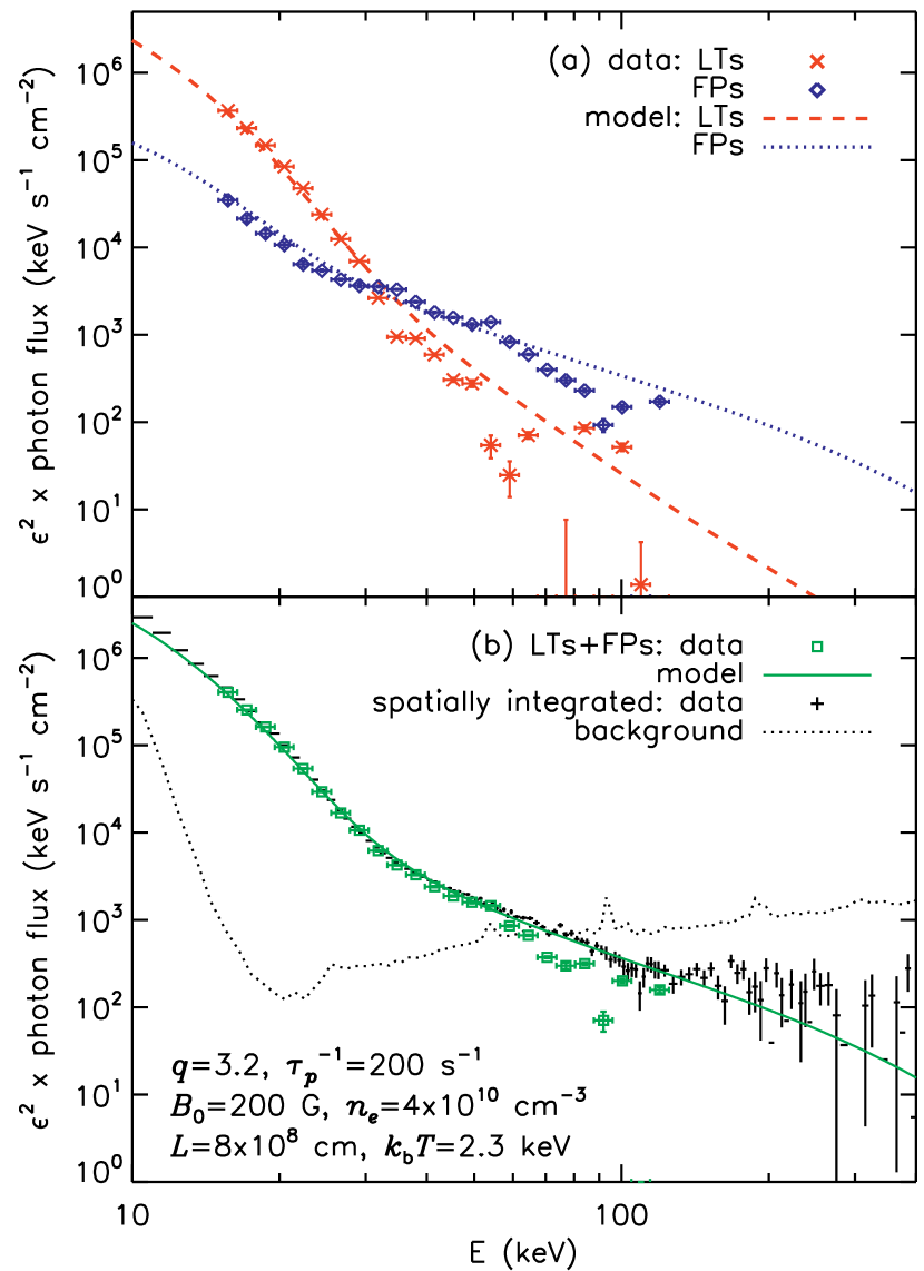
Figure 2.— Photon fluxes multiplied by energy squared ($\epsilon^{2}$) during the main HXR peak of the 2002 August 3 X1.0 flare and spectral fits using the stochastic acceleration model of PL04. (a) Summed fluxes of all LT sources and all FP sources (see Fig. 2.6 of Liu, 2006). (b) Sum (squares) of the LT and FP fluxes shown in (a) and sum (solid line) of the corresponding model fits. Overplotted are the spatially integrated spectrum (plus signs) and the corresponding preflare background (dotted line). The legend lists parameters used in the model. (We thank Siming Liu and Yan-Wei Jiang for help in producing this figure.)

Comparison between the HXRs modeled here and those observed by RHESSI satellites can serve as a unique diagnostic tool and will be pursued in a future publication. Here we show an example (Fig. 2) of how well observed LT and FP fluxes can be fitted with the above equations using a spectrum of accelerated electrons given by the PL04 model.

3. Combining Particle and Hydrodynamic Codes

The main task in this study is to combine the Stanford particle code and the NRL HD code. Here we assume that particle acceleration acts as an independent driver of the simulation and is not affected by the temperature or density evolution in the transport region of the loop. The task is thus reduced to make the transport module of the particle code and the HD code communicate interactively in real time.

3.1. Electron Heating Rate

The rate of collisional heating to the background plasma, $S_{e}$ ($\mathrm{\,ergs}\,\mathrm{\,s}^{-1}\,\mathrm{\,cm}^{-3}$), equals the rate of energy loss from the energetic electrons. This can be calculated from the electron distribution given by the transport code in two equivalent ways, the second of which is used in this study.

(1) $S_{e}$ can be evaluated from the energy loss rate ${\dot{E}}_{\rm Coul}$ due to Coulomb collisions as

$$S_{e}(s)=\int_{E_{\rm min}}^{E_{\rm max}}dE\int_{-1}^{1}f(E,\mu,s){\dot{E}}_{\rm Coul}d\mu\,,$$ (9)

where $[E_{\rm min},E_{\rm max}]$ is the range of the energy bins used in the simulation, and the electron distribution function $f(E,\mu,s)$ can be obtained from the corresponding electron flux $F(E,\mu,s)$ via equation (3).

(2) Alternatively, one can calculate the net downward energy flux carried by the electrons,

$$F_{\rm erg}(s)={a_{0}\over a(s)}\int_{E_{\rm min}}^{E_{\rm max}}dE\int_{-1}^{1}\mu EF(E,s,\mu)d\mu\,,$$ (10)

and differentiate it to obtain the net energy gain to the background plasma in a unit volume,

$$S_{e}(s)=-dF_{\rm erg}(s)/ds\,,$$ (11)

where $\mu EF(E,s,\mu)$ is the energy flux along the loop and the factor $a_{0}/a(s)$ accounts for the variation of the loop cross-sectional area. This approach is practically equivalent to equation (9), because in the HXR energy range the combination of synchrotron and bremsstrahlung radiation only constitutes a negligible fraction ($\lesssim 10^{-4}$) of the energy loss of a fast electron due to Coulomb collisions.

3.2. Code Communication

It is desirable that the particle and HD codes communicate at each time step during the time advance. The current transport code, however, can only provide a steady-state solution and does not have a time-dependent capability. This can be remedied by carefully selecting the communication time interval $\Delta t$, because particle transport occurs on a much shorter timescale than hydrodynamics. This interval should be as short as possible provided that a steady-state transport solution can be reached. By considering the electron “lifetime” (see eq. [9] of Petrosian 1973), which is determined by the energy loss time in a given loop geometry and atmospheric density distribution, Liu (2006, his §7.2.4) found the optimal interval to be $\Delta t=2\mathrm{\,s}$.

The remaining question is what heating rate the HD code should use during its time advance between adjacent communications with the particle code. Let us first change the independent variable of $S_{e}$ from distance $s$ to column depth $N(s)=\int_{0}^{s}n_{e}(s^{\prime})ds^{\prime}$,

$$S_{e}[N(s)]=S_{e}(s)/n_{e}(s)\,,$$ (12)

noting $S_{e}(s)ds=S_{e}(N)dN$ and $dN=n_{e}ds$. Here $S_{e}(N)$ is in units of $\mathrm{\,ergs}\,\mathrm{\,s}^{-1}$. We have assumed a loop of uniform cross section and thus no magnetic mirroring, and here we further neglect synchrotron loss ${\dot{E}}_{\rm synch}$ (valid for $\lesssim$1 MeV electrons). Under these assumptions, the electron flux $F[E,\mu,s(N)]\equiv F[E,\mu,N(s)]$ is a function of column depth $N$, independent of distance $s$, and so does the heating rate $S_{e}(N)$ calculated from $F(E,\mu,N)$.

The HD response timescale is characterized by sound travel time, which is 84 s for a sound speed of $166\,\mathrm{\,km}\mathrm{\,s}^{-1}$ at $T=10^{6}\mathrm{\,K}$ in a $14\mathrm{\,Mm}$ long loop here. Since $\Delta t=2\mathrm{\,s}\ll 84\mathrm{\,s}$, we assume that $S_{e}(N)$ is constant in time between adjacent code communications. During this $\Delta t$, the spatial distribution of the heating rate $S_{e}(s,t)$ varies with time merely according to the redistribution of density and thus the variation of column depth,

$$S_{e}(s,t)=S_{e}(N)n_{e}(s,t)\,.$$ (13)

In practice, at a given time $t$ and distance $s$, we first identify its column depth $N(s,t)$, which is then used to evaluate the heating rate $S_{e}(N)$, and then we apply the local density to obtain $S_{e}(s,t)$ by equation (13).

Communications between the two codes are summarized in Figure 3. First, the HD code passes the initial density distribution to the particle code, which then runs its first steady-state calculation and returns the heating rate $S_{e}(N)$ as a function of column depth to the HD code. Next the HD code repeatedly converts $S_{e}(N)$ to $S_{e}(s,t)$ as a function of distance at each time step using the latest density profile. Once the HD code advances a time interval of $\Delta t=2\mathrm{\,s}$, it passes the updated density distribution back to the particle code, which starts the next cycle of iteration.

Figure 3.— Task flow chart for communications between the particle and HD codes.

4. Simulation Runs

Table 1Summary of simulation runs.

Runs	Injected Electron		Particle	$v_{\rm max}$	$t_{v_{\rm max}}$	$v_{\rm min}$	$t_{v>100}$	$t_{\rm apex}$	$T_{\rm max}$	$n_{e,\rm max}$
	Spectrum	Ang. Distr.	Transport	($\mathrm{\,km}\mathrm{\,s}^{-1}$)	(s)	($\mathrm{\,km}\mathrm{\,s}^{-1}$)	(s)	(s)	($10^{6}\mathrm{\,K}$)	($10^{10}\mathrm{\,cm}^{-3}$)
O(ld)	power law	beamed	analy. approx.	565	35	$-115$	10	29	21.1	6.96
H(ybrid)	power law	beamed	Fokker-Planck	570	35	$-106$	9	28	22.0	7.44
N(ew)	stoch. accel.	isotropic	Fokker-Planck	598	36	$-102$	9	23	25.9	8.44

Notes. Runs O and H have an identical injected power-law electron flux, with a spectral index $\delta=6$ and low-energy cutoff $E_{c}=15\mathrm{\,keV}$; $v_{\rm max}$ and $t_{v_{\rm max}}$: maximum (upflow, $v>0$) velocity and its time stamp; $v_{\rm min}$: minimum (downflow, $v<0$) velocity (in the upper chromosphere); $t_{v>100}$: time when the upflow velocity exceeds $100\mathrm{\,km}\mathrm{\,s}^{-1}$; $t_{\rm apex}$: time when the evaporation front (density jump) reaches the loop apex; $T_{\rm max}$ and $n_{e,\rm max}$: maximum coronal temperature and electron density. All runs have the same peak energy deposition (electron heating) flux for the loop as a whole, $F_{\rm max}=2.67\times 10^{10}\mathrm{\,ergs}\mathrm{\,s}^{-1}\mathrm{\,cm}^{-2}$.

We have performed three simulation runs (see Table 1) to test the relative effects of different processes. (1) In the first run, which we refer to as the Old Model (abbreviated by “O”), we assumed an injection of electrons of a power law at the LT, and evaluated the heating rate and HD response as in the MEL89 model. This model does not calculate particle transport properly. (2) In the second simulation, we still injected power law electrons and evaluated electron transport and heating along the loop using our transport code. We call this the Hybrid Model (or “H”). (3) Finally, we employed our most realistic model, where we evaluated from our acceleration code (PL04) the spectra of electrons at the LT acceleration site and those escaping the LT region. We also calculated transport and heating using our transport code. We call it the New Model (or “N”). In all cases, we assumed an identical initial HD state as shown in Figure 1, and calculated the HD response using the MEL89 code. We assumed the dynamic or modulation profile of the number of injected electrons (power law for Runs O and H and $\dot{Q}$ for Run N) to be a triangular shape with a rise and fall to be 30 s each. Beyond this first 60 s of the impulsive phase, while the electron heating rate $S_{e}$ was set to zero, we continued the computation into the decay phase until $t=90\mathrm{\,s}$.

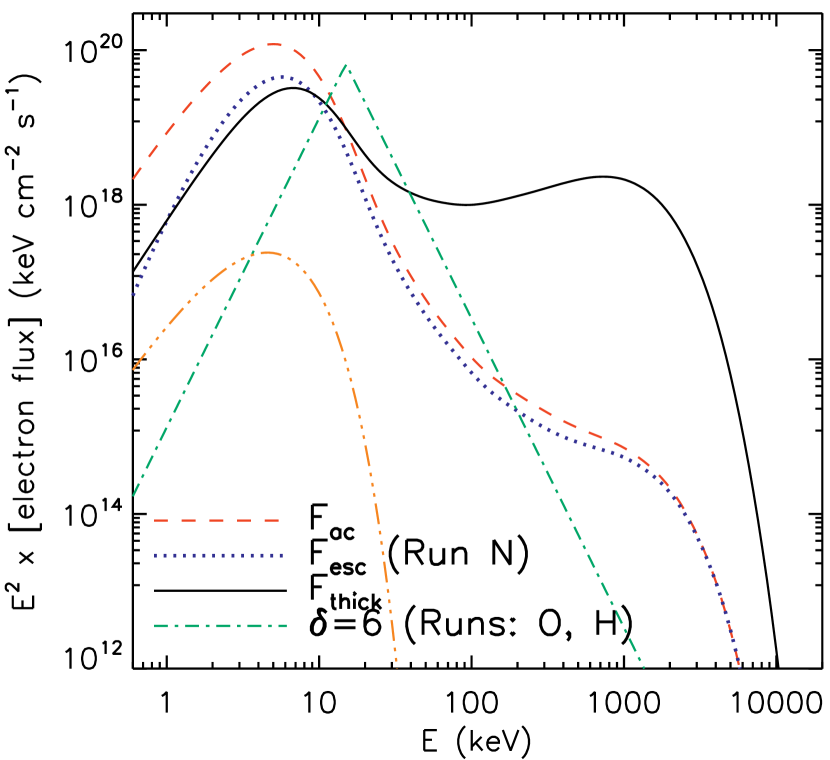
Figure 4.— Electron flux spectra $F(E)$ times $E^{2}$ at the peak time ($t=30$ s): (1) acceleration region flux $F_{\rm ac}$, escaping flux $F_{\rm esc}$, and equivalent thick-target flux $F_{\rm thick}$ for Run N, and (2) injected flux for Runs O and H ($\delta=6$ above $E_{c}=15$ keV). The triple-dot-dashed line (arbitrary scale) represents the source term $\dot{Q}(E)$ of a Maxwellian (thermal, $k_{b}T=1.53\mathrm{\,keV}$) distribution used in Run N, which peaks at $E=3k_{b}T$ in this $E^{2}F(E)$ plot.

4.1. Run O: Old Model

We first computed the HD response using the same heating function and almost identical control parameters as the “Reference Calculation” of MEL89. This model is based on the analytical solution of Emslie (1978) that includes only energy loss and pitch angle growth of injected electrons. By the MEL89 assumption, the injected electron flux is downward beamed ($\mu_{0}=1$), and its energy spectrum (see Fig. 4) is a broken power law $\propto E^{-\delta}$ with an index $\delta=6$ above and $\delta=-2$ below the cutoff (“knee”) energy $E_{c}=15$ keV. Here the differences are: (1) our peak energy flux, i.e., parameter $F$ in equation (9) of MEL89, is $2.67\times 10^{10}\mathrm{\,ergs}\mathrm{\,cm}^{-2}\mathrm{\,s}^{-1}$, while they used $5\times 10^{10}\mathrm{\,ergs}\mathrm{\,cm}^{-2}\mathrm{\,s}^{-1}$, and (2) we assume a fully ionized hydrogen plasma while they included helium of 6.3% of hydrogen in number density. The latter difference only changes the absolute mass density by 11%, while the relative differences between our models may not be affected.

4.2. Run H: Hybrid Model

Here we used our Fokker-Planck transport code in place of the approximate analytical expression used above to evaluate the heating rate. We injected electrons of an identical power-law spectrum with a narrow-Gaussian ($\sigma_{\mu}=0.01$) pitch-angle distribution to emulate the beamed distribution in Run O. The main difference here is that the transport code properly treats the diffusion process of pitch angle change due to Coulomb collision. For the particle code, the energy space is divided into 200 uniform logarithmic bins in the range of $511\times[10^{-3},10^{3}]$ keV, while the pitch angle space is divided into 100 (vs. 24 used in Liu, 2006) uniform bins in the $[0,\pi]$ range.

4.3. Run N: New Model

This is a typical simulation using our new model. It is the same as Run H, except that the injected beamed power-law electron flux is replaced with an isotropic flux given by the stochastic acceleration code. We used the same acceleration parameters as PL04 (see their Fig. 12), i.e., the characteristic acceleration rate $\tau_{p}^{-1}=70\mathrm{\,s}^{-1}$, $n_{e}=1.5\times 10^{10}\mathrm{\,cm}^{-3}$, $B_{0}=400\mathrm{\,G}$, $k_{b}T=1.53\mathrm{\,keV}$, and the acceleration region size $L=5\times 10^{8}\mathrm{\,cm}$. We modulated the rate ($\dot{Q}$, see eq. [1]) of electrons being supplied to the acceleration region with the same triangular time profile, such that the peak electron heating flux $F_{\rm max}$ equals that of Run O or H.

Figure 4 shows various electron flux spectra used in this study. In comparison with the background thermal distribution, both the acceleration region flux $F_{\rm ac}$ and escaping flux $F_{\rm esc}$ have a quasi-thermal component that smoothly extends to a nonthermal tail at high energies. $F_{\rm esc}$ is smaller than $F_{\rm ac}$ and their relative difference decreases with energy due to the energy-dependent confinement of electrons by turbulence in the acceleration region (see eq. [2]). Unlike that (dot-dashed) in Run O or H, the flux $F_{\rm esc}$ injected into the transport region does not invoke any arbitrary low-energy cutoff. The two fluxes, however, have similar slopes in the intermediate energy range around 20 keV. The equivalent thick-target electron flux $F_{\rm thick}$ (see §2.4), as expected, has a harder spectrum than $F_{\rm ac}$ and $F_{\rm esc}$ in the 10–1000 keV range.

5. Simulation Results: Comparison of Fluid Dynamics

To determine how much our proper transport and acceleration calculations affect the atmospheric response, we compare the results of the three simulations, using Run H as the reference case.

5.1. Hydrodynamic Evolution

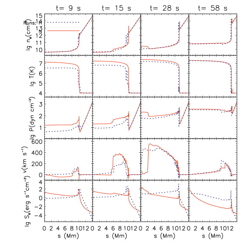
Figure 5.— Evolution of electron density, temperature, pressure, velocity, and electron heating rate for Runs H and N.

As shown in Figure 5, Run H exhibits similar general HD evolution as described in MEL89 (their Figs. 1 and 2). Electron heating ($S_{e}$) is initially concentrated in the upper chromosphere, producing overpressure that drives an upflow ($v>0$) and a recoil downflow ($v<0$). At $t=9\mathrm{\,s}$, the upflow velocity exceeds $100\mathrm{\,km}\mathrm{\,s}^{-1}$ and a density jump or evaporation front has developed slightly above the TR. It travels upward and reaches the loop apex at $t=28\mathrm{\,s}$. The density jump is then reflected back and the material piles up due to the reflective boundary condition imposed, which can be understood as plasma flow from the other half of the loop in the assumed symmetric geometry. The upflow reaches its maximum velocity of $v_{\rm max}=570\mathrm{\,km}\mathrm{\,s}^{-1}$ at $t=35\mathrm{\,s}$, which is delayed by 5 s from the energy deposition peak at $t=30\mathrm{\,s}$. Chromospheric evaporation then gradually subsides. These features of the temporal evolution can also be seen from the history of various quantities at a fixed position in the upper corona as shown in Figure 6. Note that, late during the simulation, the coronal temperature gradually decreases mainly due to conductive cooling, while the coronal density continues to increase, even after the cease of electron heating at $t=60\mathrm{\,s}$. This is caused by sustained chromospheric evaporation that results from heating of the chromosphere by the same conductive flux that cools the hot corona.

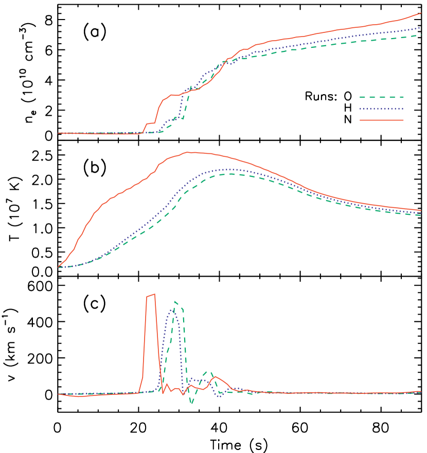
Figure 6.— History of electron density, temperature and velocity at $s=1$ Mm from the injection site for different simulations.

In comparison, we find that Run O is very similar to Run H (see Fig. 6 and Table 1) but less intense. This can be more clearly seen from various HD quantities and heating and cooling rates during the early phase shown in Figure 7. The small differences (on the order of 10%) between the two cases are mainly caused by the slight overestimate of electron heating of Run O in the chromosphere (Fig. 7d), due to its inaccurate way of calculating particle transport noted earlier. This indicates that, for this specific case, the analytical heating function used in MEL89 provides an acceptable approximation for the more accurate Fokker-Planck calculation.

In contrast, the HD evolution of Run N is faster and more intense than that of Run H (Figs. 5 and 6, Table 1), despite the same maximum electron heating rate for the two cases. These differences are primarily due to the different energy spectra of injected electrons, further enhanced by their different pitch-angle distributions:

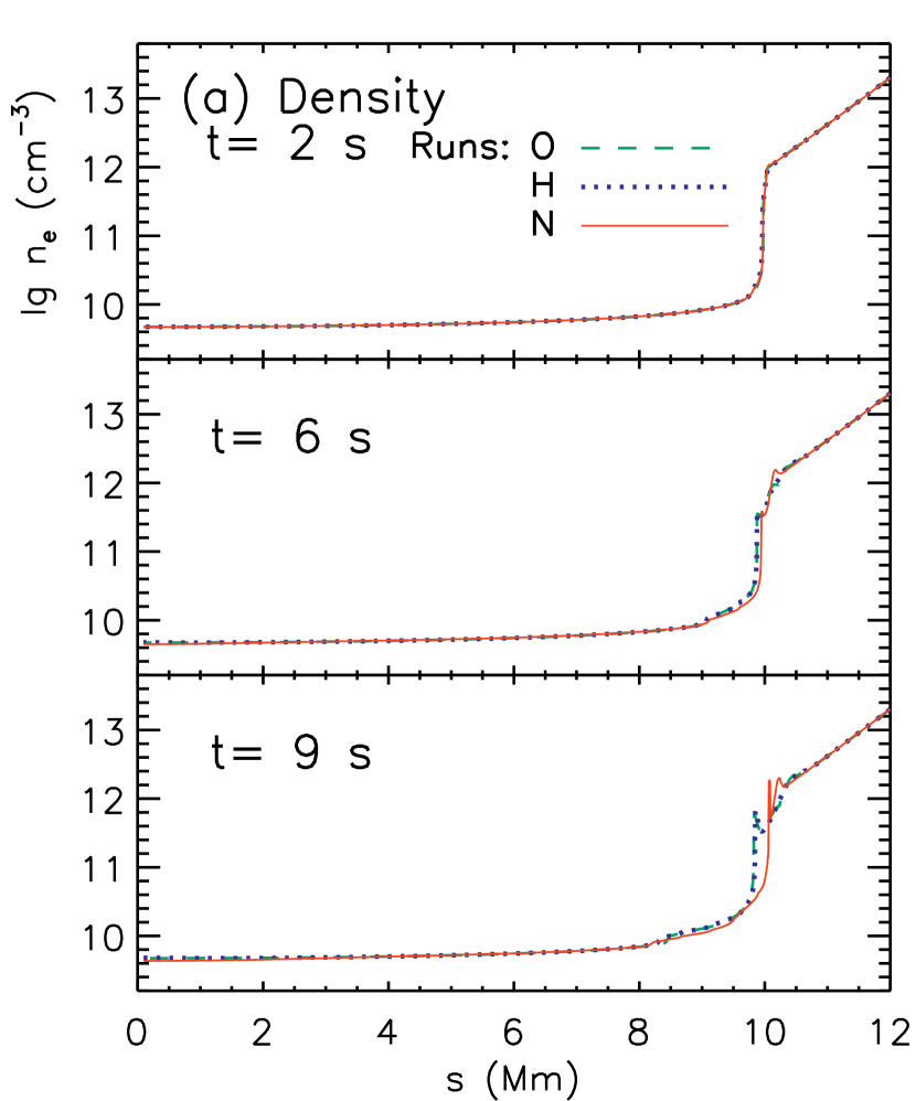
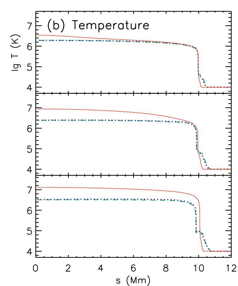
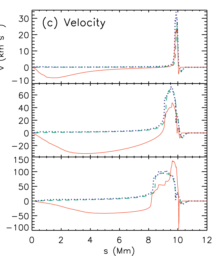
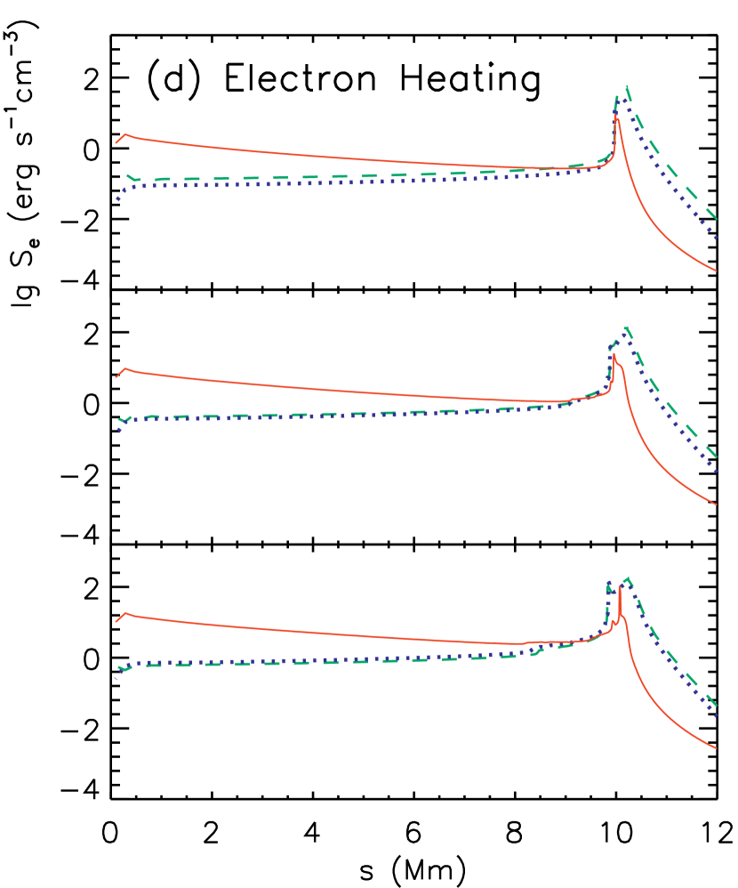
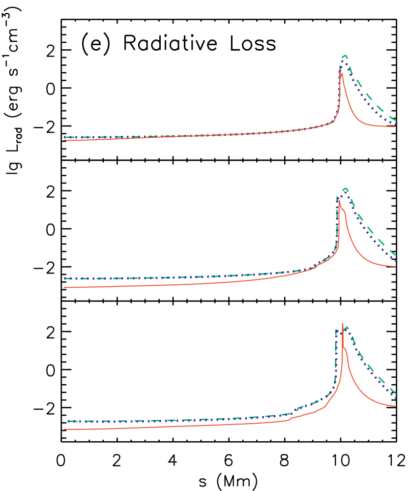
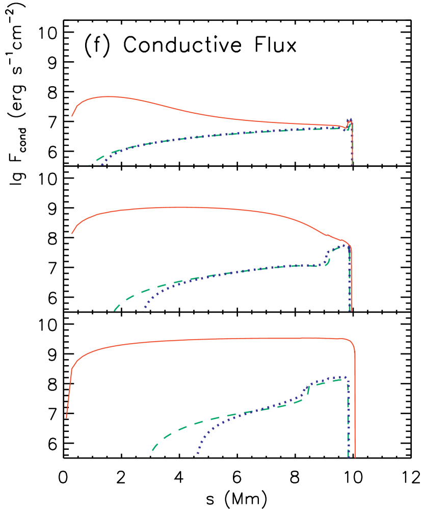
Figure 7.— Same as Fig. 6 but for snapshots of various quantities as a function of distance at selected times early in the flare.

(1) In Run N, electrons of a few keV in the quasi-thermal component of the spectrum (Fig. 4) are small in energy but large in number and thus dominate the total energy content. These electrons produce heating at relatively small column depths by Coulomb collisions. This occurs high in the corona (Fig. 7d), where the radiative loss rate $L_{\rm rad}$ (Fig. 7e) is relatively small due to the low density and high temperature. As a result, significant net heating sets in there, which leads to a local temperature (Fig. 7b) and pressure surge. This local coronal heating is enhanced by the large effective column depth ($N_{\rm eff}=N/\langle\mu\rangle$, where $\langle\mu\rangle$ is the mean pitch angle cosine) resulting from the isotropic pitch-angle distribution of the injected electrons. The increased temperature leads to a large downward heat conduction flux (Fig. 7f), and the pressure gradient force drives a downward mass flow in the high corona (Fig. 7c).

(2) In Run H, contrastingly, the electron spectrum (Fig. 4) peaks at the cutoff energy $E_{c}$, which leads to a deficit in low-energy electrons. In addition, the pitch-angle distribution here is beamed (rather than isotropic). This electron population, on average, penetrates deeper into the atmosphere than that in Run N and deposit their energy primarily in the upper chromosphere. This results in less heating in the corona and stronger and more widespread heating in the chromosphere (Figs. 7b and 7d). Consequently, in spite of the larger and broader radiative cooling (Fig. 7e), the local overpressure in the chromosphere is stronger than that in Run N early on, which drives a higher velocity upflow (Fig. 7c, $t=6\mathrm{\,s}$). Also, unlike Run N, there is no significant downward coronal heat conduction (Fig. 7f) or mass flow.

5.2. Heating and Cooling

A remaining question is why Run N has more dramatic overall HD changes in the long run. To answer this, we examine the relationship between different energy gain and loss terms — electron heating, radiative loss, and conductive heating and cooling — particularly early in the flare and near the TR where chromospheric evaporation takes place.

(1) In Run N at $t=1\mathrm{\,s}$ (see top panel of Fig. 8a), the electron heating rate $S_{e}$ peaks in the TR because of the sharp increase there in ambient density and associated collisional energy loss of energetic electrons. So does the radiative loss rate $L_{\rm rad}$, since it is proportional to $n_{e}n_{p}$ and $\Phi(T)$ that peaks at $T\simeq 1-3\times 10^{5}\mathrm{\,K}$ which is the TR temperature. However, due to their different functional dependencies on density and temperature, $S_{e}$ peaks at a slightly lower position than $L_{\rm rad}$. Their combination $S_{e}-L_{\rm rad}$ (panel 2, Fig. 8a) thus results in cooling in the upper TR and heating in a shallow layer below it in the upper chromosphere. Meanwhile, the conductive flux carries energy from the hot upper corona to the upper TR where localized heating ($S_{\rm cond}$) is produced and counteracts radiative cooling. (Conduction is prohibited in the chromosphere where the temperature is maintained at $10^{4}\mathrm{\,K}$.) The net energy gain resulting from the interplay of electron heating, radiative cooling, and heat conduction is thus localized in the upper chromosphere, where temperature is raised substantially (panel 3, Fig. 8a). This leads to a local pressure hump which drives an upflow into the corona and a downflow into the chromosphere (panel 4, Fig. 8a).

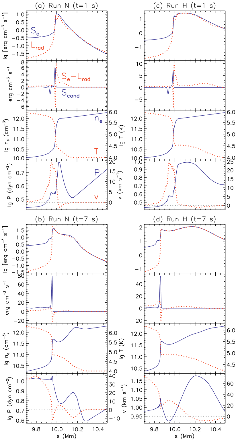
Figure 8.— Comparison between Runs N (left) and O (right) of a detailed view near the TR at two selected times. At each time, the quantities in the four panels (from top to bottom) are: (1) electron heating rate $S_{e}$ and radiative loss rate $L_{\rm rad}$, (2) $S_{e}-L_{\rm rad}$ (dotted) and conductive heating rate $S_{\rm cond}$ (solid), (3) electron density (left scale) and temperature (right scale), and (4) pressure (left) and velocity (right). Note different vertical scales.

As time proceeds (see Fig. 8b) and chromospheric material is being heated from $T=10^{4}\mathrm{\,K}$ to $\sim$$10^{5}\mathrm{\,K}$ where $\Phi(T)$ reaches its maximum, radiative loss gradually overtakes electron heating in the TR and upper chromosphere. This means that energy directly deposited by electrons in these places is immediately radiated away and very little is left to heat the plasma. However, as we noted above, a significant portion of the energy content of the injected electrons in Run N is deposited in the upper corona (Fig. 7d) where radiative loss is negligible and then transported by heat conduction to the lower atmosphere. In time, conduction plays an increasingly important role in heating the lower corona and TR as it gradually exceeds the direct net heating or combined electron heating and radiative loss $S_{e}-L_{\rm rad}$ (Fig. 8b) in these regions. Because of this, as of $t=7\mathrm{\,s}$ the location of the primary net heating, i.e., the highest local overpressure, and the maximum downflow velocity have shifted from the upper chromosphere up to the TR. In fact, the peak of the conductive flux $F_{\rm cond}$ (see Fig. 7f) and the region of significant conductive heating ($S_{\rm cond}\propto-dF_{\rm cond}/ds$) below it are initially located in the upper corona and propagate down the loop with time. As the $F_{\rm cond}$ peak approaches the TR at $\sim$10 Mm during the interval of 8–10 s, the maximum upflow velocity $v_{\rm max}$ in the loop increases abruptly (see Fig. 9). This further emphasizes the role played by heat conduction here in redistributing energy deposited by electrons and in driving chromospheric evaporation.

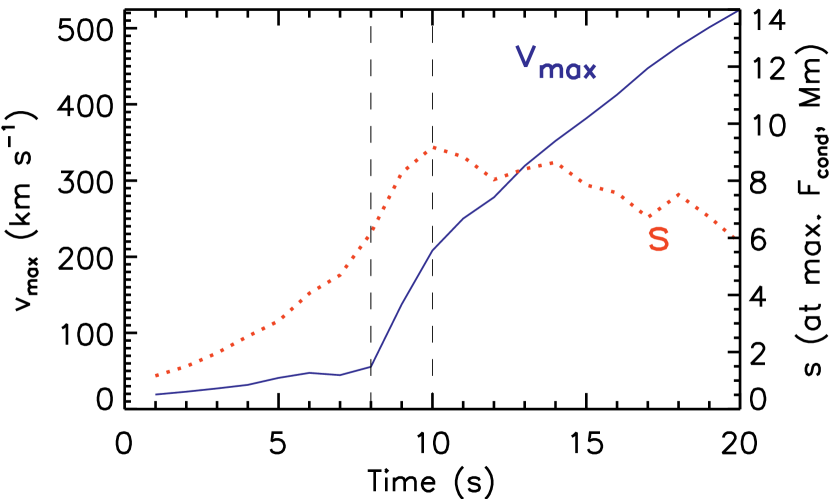
Figure 9.— Early history of the maximum upflow velocity $v_{\rm max}$ (left scale) and the position of the maximum conductive flux (right scale) for Run N. The two vertical lines mark the interval when $v_{\rm max}$ experiences a sharp increase while the maximum $F_{\rm Fond}$ rapidly approaches the TR.

(2) In Run H, the injected electron flux with a low-energy cutoff has profound consequences. As noted earlier, lack of low-energy electrons makes the chromosphere, rather than the upper corona, the primary location of direct heating early in the flare (see Fig. 7d). Net direct heating $S_{e}-L_{\rm rad}$ and the increase of local temperature and pressure extend from the TR to much deeper layers of the chromosphere than in Run N (Fig. 8c). Moreover, since the coronal temperature does not increase rapidly, the downward conductive flux here is more than an order of magnitude smaller (Fig. 7f). Net direct heating generally dominates over conductive heating when integrating over the volume of the lower atmosphere. As a result, in comparison with Run N, a relatively larger portion of the total energy content of the injected electrons is lost in radiative cooling. This is why the overall HD development here is more gentle than that of Run N, despite the fact that they have the same energy deposition flux. The primary underlying physics is their different spatial distributions of electron heating $S_{e}$ caused by their different electron injections. Note that MEL89 obtained qualitatively similar results when different values of the cutoff energy or spectral index were considered. We note that, later during the impulsive phase in Run H (Fig. 5), as the coronal density has increased considerably due to chromospheric evaporation, relatively more electron energy is directly dumped in the corona while less in the chromosphere. Consequently, conductive heating in the TR becomes important. In this sense, the physical distinction between the two runs gradually diminishes in the late stage of the flare.

5.3. Velocity Distribution

Here we examine observables that can be checked against data: (1) the temperature dependence of the plasma velocity (Fig. 10, left), and (2) the velocity differential emission measure (VDEM; Fig. 10, right) defined by Newton et al. (1995) as the emissivity ($G[T]$) weighted measure of material with line-of-sight (LOS) velocity $v_{\rm LOS}$. Assuming that the flare is located at the solar disk center such that the LOS is perpendicular to the loop apex, we calculated the specific VDEM/$a(s)$ for the Ca XIX 3.18 Å line following Newton et al. Here $G(T)$ is given by the Chianti package (Young et al., 2003).

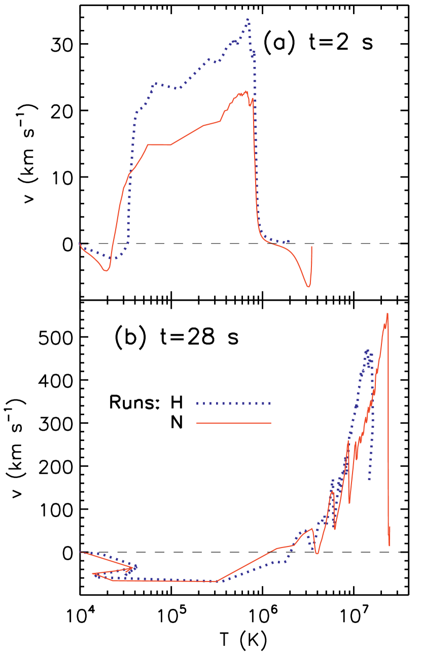
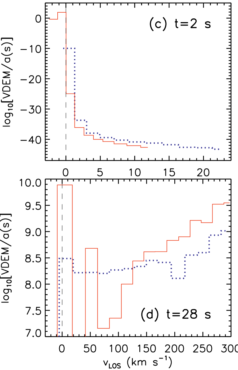
Figure 10.— Comparison between Runs H and N: velocity vs. temperature (left) and corresponding specific velocity differential emission measure (photons $\mathrm{\,cm}^{-2}\,\mathrm{\,s}^{-1}\,{\rm sr}^{-1}\,[\mathrm{\,km}\,\mathrm{\,s}^{-1}]^{-1}$) vs. LOS velocity (right).

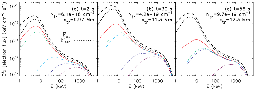
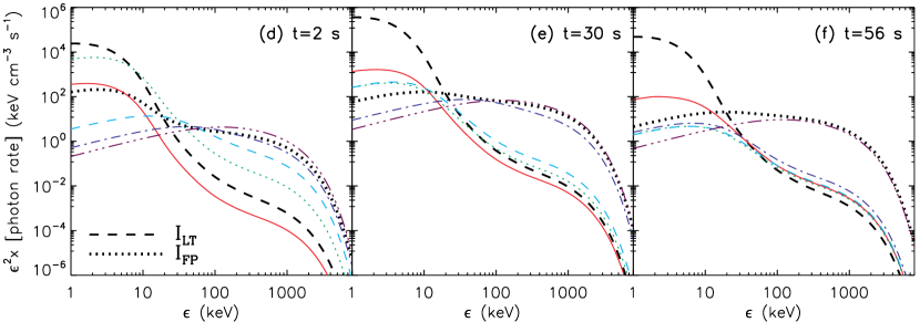
Figure 11.— Spectra of angle-integrated electron flux (top) and corresponding photon emission rate (bottom) multiplied by energy squared at three selected times for Run N. The thick dashed line represents the LT (acceleration region) spectrum ($F_{\rm ac}$ or $I_{\rm LT}$), while the thin colored lines (solid, dotted, dashed, dot-dashed, and triple-dot–dashed) are the spectra at distances $s=$ 4, 10, 11, 12, and 13 Mm from the injection site. The thick dotted line indicates the escaping electron flux ($F_{\rm esc}$) in the top panels and the equivalent FP photon emission rate ($I_{\rm FP}$) in the bottom panels. The legends show the current values of the position ($s_{\rm tr}$) and column depth ($N_{\rm tr}$) of the TR.

Early in the flare (Figs. 10a and 10c), Run H has higher upflow velocities and downflow temperatures than Run N, owing to its stronger net direct heating with a deeper extent in the chromosphere (Fig. 8c). Run N has an additional hot downflow component at $\gtrsim$2 MK, due to the expansion of the heated upper corona mentioned earlier. This hot component also dominates the VDEM at $v_{\rm LOS}<0$ (Fig. 10c) because of the sharp rise of $G(T)$ up to $T=29\mathrm{\,MK}$. Later at $t=28\mathrm{\,s}$ (Fig. 10b), Run N overtakes H in upflow velocity and temperate, while its hot coronal downflow has disappeared. Run N has a bimodal VDEM (Fig. 10d) with a strong stationary, hot component located near the loop apex (also see Fig. 5), while Run H exhibits a more gradual progression toward high velocities. This distinction is similar to what Newton et al. (1995, see their Fig. 2) found for models with different initial coronal densities.

6. Effects of Hydrodynamics on Particle Transport and X-ray Emission

We now turn our attention to the effects of fluid dynamics on particle characteristics, namely, electron transport and nonthermal radiation. Here we present the result of Run N as a typical example. We will examine first the energy distributions of electrons and bremsstrahlung photons, and then their spatial distributions.

6.1. Electron and Photon Energy Spectra

Figure 11 (top panels) shows the evolution of the angle-integrated electron flux spectrum $E^{2}F(E,s)$ at different locations in the loop. In general, at a given time and a moderately large distance or column depth, there is a deficit in low-energy electrons due to collisional energy losses and scatterings on the paths of the electrons from the injection site. This appears as a turnover in the spectrum and slight spectral hardening just above the turnover energy. As distance increases, progressively more low-energy electrons are lost, and thus the overall flux decreases while the spectral turnover shifts to higher energies (Leach & Petrosian, 1981). At $t=2\mathrm{\,s}$ (Fig. 11a) the TR is located at distance $s_{\rm tr}=9.97\mathrm{\,Mm}$ and column depth $N_{\rm tr}=6.1\times 10^{18}\mathrm{\,cm}^{-2}$. The two fluxes at $s=4$ and 10 Mm (thin solid, dotted) are located in the low-density corona or TR at small column depths from the injection site, and thus appear similar in shape to the escaping flux $F_{\rm esc}$ (thick dotted). Other fluxes at $s=11$, 12, and 13 Mm are located in the chromosphere at large column depths, and thus exhibit substantial reduction of low-energy electrons.

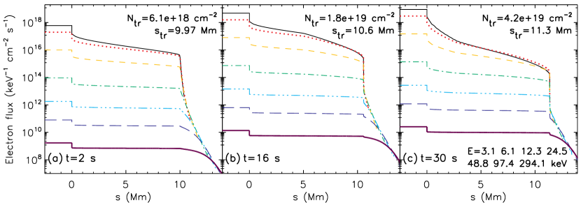
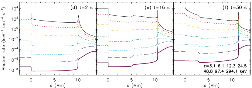
Figure 12.— Spatial distributions of angle-integrated electron flux (top) and photon emission rate (bottom) at three selected times for Run N. From top to bottom, different lines in each panel represent electron or photon energies of 3.1, 6.1, 12.3, 24.5, 48.8, 97.4, and 294.1 keV. The step in the $s<0$ region corresponds to one half length of the acceleration region at the top of the loop (see Fig. 1). The step at the TR is due to the jump in the ambient density.

In this study, the flux ($F_{\rm esc}$) injected into the transport region does not change with time in spectral shape but only varies in normalization. So does the electron flux at a given column depth. However, as chromospheric evaporation develops, the TR retreats to lower altitudes (Fig. 5), while the coronal density increases. This causes the change of the column depth and thus the electron spectrum at a fixed location, which is what we notice here. At $t=30\mathrm{\,s}$ (Fig. 11b) when the TR shifts down to $s_{\rm tr}=11.3\mathrm{\,Mm}$ at $N_{\rm tr}=4.2\times 10^{19}\mathrm{\,cm}^{-2}$, the spectrum at $s=11$ Mm looks similar to the other coronal spectra (at $s=4$ and 10 Mm) but different from the chromospheric spectra. Meanwhile, the relative difference between the first coronal spectrum ($s=4$ Mm) and the injected spectrum $F_{\rm esc}$ becomes larger, because of the increasing coronal density and column depth between them. This trend continues through the end of the simulation.

The bottom panels of Figure 11 show the corresponding bremsstrahlung photon spectra $\epsilon^{2}I(\epsilon,s)$ defined in equation (7). Like its electron counterpart, the LT photon spectrum $\epsilon^{2}I_{\rm LT}$ (thick dashed) shows a thermal-like component at low energies and a nonthermal tail at intermediate energies with a cutoff at high energies. The equivalent FP spectrum $\epsilon^{2}I_{\rm FP}$ below $s_{\rm tr}$ (thick dotted, defined in §2.4) is harder than the LT spectrum. Their shapes in the 10s–100s keV range are commonly observed for LT and FP sources. At larger distances, the spectra (thin lines) become progressively harder because the corresponding electron spectra have the same variation (Leach & Petrosian, 1983) as we have noticed above, and high-energy ($>$10s keV) emission increases because of higher ambient densities. As the coronal density increases with time, for the same reason mentioned above photon spectra at positions originally located in the corona become progressively harder. At the same time, as the TR treats, spectra at positions originally in the chromosphere but now in the corona become softer. In other words, the difference in spectral shape between X-ray emissions at different positions diminishes with time (Figs. 11e and 11f).

6.2. Electron and Photon Spatial Distributions

Figure 12 (top panels) shows the evolution of the angle-integrated electron flux $F(E,s)$ as a function of distance at different energies from 3 to $300\mathrm{\,keV}$. The step at $s=0$ is owing to the difference between the LT (acceleration region) flux $F_{\rm ac}$ and the escaping flux $F_{\rm esc}$ mentioned before (see Fig. 4). In general, the electron flux decreases with distance or column depth from the injection site. The slope of the curve $-dF(E,s)/ds$ is steeper at lower energies because lower energy electrons lose energy faster and are more sensitive to pitch-angle scattering. At a given energy, the slope depends on the ambient density, because $dF(E,s)/ds=n_{e}[dF(E,N)/dN]$, where $F(E,N)$ is generally a smooth function of $N$ (McTiernan & Petrosian, 1990). Therefore, if there is a rapid increase in density with distance, the slope increases quickly; the opposite would be true if the density were to decrease sharply. A sharp break is obvious at the TR, and a milder break occurs at the evaporation front (e.g., at $s\simeq 5\mathrm{\,Mm}$ in Fig. 12b). An upward break or flattening is visible at $s\simeq 3\mathrm{\,Mm}$ where the density jump is reflected back from the loop apex at $t=30\mathrm{\,s}$ (Fig. 12c). It is also visible just below the TR (see Figs. 12b and 12c), where a sharp density decrease from the narrow density spike occurs (Fig. 5). As density increases due to chromospheric evaporation, the spatial distribution in the corona becomes steeper. The slope variation with distance (i.e., breaks) and time is more pronounced at lower energies for the same reason noted above.

Figure 12 (bottom panels) shows the evolution of the corresponding spatial distribution of angle-integrated bremsstrahlung emission $I(\epsilon,s)$. In the early stage, low-energy emission comes primarily from the LT, while high-energy emission is concentrated below the TR. Because nonthermal bremsstrahlung radiation is proportional to both the electron flux and local target density, photon emission reflects details of the density distribution in a more pronounced way than the electron flux profile. As is evident, the emission profile clearly indicates density features, including the evaporation front and the density spike just below the TR. The local emission enhancement at the evaporation front moves upward with time, which may be responsible for the observed X-ray sources moving along the loop (Liu et al., 2006b; Sui et al., 2006) mentioned in § 1.1. As time proceeds, relatively more emission comes from the coronal portion of the loop because of the increased density. Specifically, at low energies, the emission intensity decreases with distance in the corona more sharply than before. At intermediate energies, we find a temporal transition from FP-dominated emission to LT-dominated emission, which occurs at progressively higher energies, reminiscent of the phenomenon observed by Liu et al. (2006b). At high energies, such a change is not visible because the high density corona still looks transparent to high-energy electrons, but the retreat of the TR is obvious.

7. Summary and Discussion

We have performed simulations of solar flares that self-consistently combine acceleration, transport, and radiation of energetic electrons (using the Stanford unified code) with fluid dynamics of the atmospheric response (using the NRL flux tube code). As the first successful one of its kind, this model improves on previous HD simulations in two major aspects. First, it includes more accurate evaluation of electron heating from full Fokker-Planck calculation of particle transport. Second, it uses a more realistic electron spectrum from the stochastic acceleration model (PL04) as the injection to the transport region. We compare this more advanced treatment with models in which an ad hoc electron distribution of a power-law with a low-energy cutoff is injected into the loop and/or transport is dealt with approximately. Our conclusions are:

1. For the specific injection of beamed, power-law electrons, the old analytical model of MEL89 (Run O) provides an acceptable approximation. Its result differs by $\sim$10% from that of the reference hybrid model (Run H) obtained by the more accurate Fokker-Planck calculation (see Table 1 and Figs. 6 and 7).

2. In the new model (Run N), where the injected electron spectrum is based on stochastic acceleration, we find higher coronal temperatures and densities, larger upflow velocities, and faster increases of these quantities than the hybrid model (Run H, Fig. 6). This is mainly because the new injected electron spectrum smoothly spans from a quasi-thermal component to a nonthermal tail (Fig. 4). The low-energy electrons in the quasi-thermal regime, which contain the bulk of the total energy budget, deposit their energy primarily in the corona. This results in significant coronal heating and thus a large downward heat conduction flux that helps drive “evaporation” of plasma at the TR. In contrast, the electron spectrum in the hybrid model with a low-energy cutoff leads to more energy directly deposited in the chromosphere, which is radiated away more quickly, leaving less energy to produce actual heating (Figs. 7 and 8). This is qualitatively consistent with the conclusion of MEL89 where an electron spectrum with a smaller low-energy cutoff or steeper slope resulted in a stronger chromospheric evaporation.

3. The energy and spatial distributions of energetic electrons and bremsstrahlung photons bear the fingerprint of the changing density distribution caused by chromospheric evaporation. In general, as time proceeds, the electron and photon spectra at positions remaining in the corona become progressively harder because of the increasing coronal density, while those at positions previously in the chromosphere and now in the corona (due to the retreat of the TR) become softer (Fig. 11). Any density jump in space results in a sudden change in the spatial distributions of energetic electrons and X-ray photons (Fig. 12). In particular, the evaporation front appears as a local emission enhancement, which, in principle, can be imaged by X-ray telescopes.

7.1. Comparison with Observations

Over several decades (see review by Antonucci et al., 1999), Doppler observations have indicated hot, fast ($\gtrsim$$100\mathrm{\,km}\mathrm{\,s}^{-1}$) upflows (Doschek et al., 1980) and cool, slow ($\gtrsim$$10\mathrm{\,km}\mathrm{\,s}^{-1}$) downflows (Wuelser et al., 1994; Brosius & Phillips, 2004) during flares. This is consistent with chromospheric evaporation and momentum recoil shown in our and earlier simulations (e.g., Mariska et al., 1982; Fisher et al., 1985c). In addition, Milligan & Dennis (2009) reported plasma velocities at multiple temperatures obtained from Hinode EUV Imaging Spectrometer (EIS) observations, which show excellent agreement with the Run N curve in Figure 10b throughout the $10^{4}$–$10^{7}$ K range. Such an agreement with HD simulations has not been seen before.

Heat conduction, compared with more popular direct electron heating, plays an important role in driving chromospheric evaporation in our new model. Observational support of this was first reported by Zarro & Lemen (1988), who found an upflow velocity $\lesssim 50\mathrm{\,km}\mathrm{\,s}^{-1}$ at $T\simeq 6\mathrm{\,MK}$ during the cooling phase of a flare. Milligan (2008) recently reported an unusually high temperature (2 MK) downflow at $\sim$$14\mathrm{\,km}\mathrm{\,s}^{-1}$ in a microflare with no detection of HXRs (implying a low flux of nonthermal electrons), which possibly results from conductive heating. This downflow could be due to the thermal expansion early in the corona (Fig. 10a) or the momentum recoil later in the chromosphere (Fig. 10b). More recently, Battaglia et al. (2009) interpreted the growths of the SXR emission measure observed early during flares (before HXRs being observed) as new evidence of conduction-driven chromospheric evaporation.

Our simulations predict that evaporation upflows tend to have higher temperatures when conductive heating dominates over direct electron heating, while the opposite is true for recoil downflows (Fig. 10). This can be checked against observed distributions of the plasma bulk velocity vs. temperature (e.g., Milligan & Dennis, 2009). Our simulated VDEM can also be readily used to synthesize emission lines (Newton et al., 1995) to be compared with observations and help differentiate theoretical models, because of the sensitive dependence of VDEM on heating mechanisms.

7.2. Future Work

This paper is the first in a series and we have established the numerical model and presented initial results. In followup papers, we will explore the parameter space and use this model to investigate the Neupert effect and the observed moving X-ray sources (Liu et al., 2006b; Sui et al., 2006). More importantly, we will incorporate the atmospheric feedback on the acceleration process. This is because chromospheric evaporation may change the physical condition (e.g., plasma density and temperature) in the LT acceleration region. The density enhancement, for example, causes the ratio of electron plasma frequency to gyro-frequency $\alpha=\omega_{\rm pe}/\Omega_{e}\propto n_{e}^{1/2}/B_{0}$ to increase. This can lead to the reduction of the efficiency of electron acceleration (PL04) and thus the quenching or spectral softening (e.g., Parks & Winckler, 1969) of nonthermal HXR tails observed during the late stages of flares.

Some technical aspects of this model can be improved in the future: (1) The fully ionized hydrogen plasma assumed here can be replaced by a plasma of a more realistic solar abundance, with the inclusion of neutrals and ionization equilibrium. (2) The “cold” target assumption in the transport code can be abandoned and replaced with Coulomb diffusion in energy space (Spitzer, 1962; Miller et al., 1996) for a general “warm” target plasma (Emslie, 2003). (3) In particle transport and HD calculations, one can include energetic protons (c.f., Emslie et al., 1998) and heavier ions, whose momentum loss to the background plasma, in addition to the overpressure (Kosovichev, 2006) produced by electron heating, could contribute to generating seismic waves observed in some flares (Kosovichev & Zharkova, 1998; Donea & Lindsey, 2005). (4) In the long run, we intend to implement time-dependent particle transport calculation, full loop simulation in an asymmetric geometry, return currents, and radiative transfer.

The combined treatment of the particle and fluid descriptions of plasma presented here opens a door to a broad range of applications. This model, with proper modifications, can be applied to environments where interrelated particle acceleration and transport and plasma flows are present, such as (exo)planetary auroras (e.g., Liu & Airapetian, 2008) and flares on other stars and in accretion disks near black holes.

References

- Abbett & Hawley (1999) Abbett, W. P. & Hawley, S. L. 1999, ApJ, 521, 906
- Allred et al. (2005) Allred, J. C., Hawley, S. L., Abbett, W. P., & Carlsson, M. 2005, ApJ, 630, 573
- Antonucci et al. (1999) Antonucci, E., Alexander, D., Culhane, J. L., de Jager, C., MacNeice, P., Somov, B. V., & Zarro, D. M. 1999, in The Many Faces of the Sun: A Summary of the Results from NASA’s Solar Maximum Mission, ed. K. T. Strong et al. (New York: Springer-Verlag), 345
- Bai & Ramaty (1978) Bai, T. & Ramaty, R. 1978, ApJ, 219, 705
- Battaglia et al. (2009) Battaglia, M., Fletcher, L., & Benz, A. O. 2009, accepted by A&A
- Brosius & Phillips (2004) Brosius, J. W. & Phillips, K. J. H. 2004, ApJ, 613, 580
- Brown (1971) Brown, J. C. 1971, Sol. Phys., 18, 489
- Brown (1973) —. 1973, Sol. Phys., 31, 143
- Chandrashekar & Emslie (1987) Chandrashekar, S. & Emslie, A. G. 1987, Sol. Phys., 107, 83
- Chang & Cooper (1970) Chang, J. S. & Cooper, G. 1970, Journal of Computational Physics, 6, 1
- Donea & Lindsey (2005) Donea, A.-C. & Lindsey, C. 2005, ApJ, 630, 1168
- Doschek et al. (1980) Doschek, G. A., Feldman, U., Kreplin, R. W., & Cohen, L. 1980, ApJ, 239, 725
- Dung & Petrosian (1994) Dung, R. & Petrosian, V. 1994, ApJ, 421, 550
- Emslie (1978) Emslie, A. G. 1978, ApJ, 224, 241
- Emslie (2003) —. 2003, ApJ, 595, L119
- Emslie et al. (1992) Emslie, A. G., Li, P., & Mariska, J. T. 1992, ApJ, 399, 714
- Emslie et al. (1998) Emslie, A. G., Mariska, J. T., Montgomery, M. M., & Newton, E. K. 1998, ApJ, 498, 441
- Emslie & Nagai (1985) Emslie, A. G. & Nagai, F. 1985, ApJ, 288, 779
- Fisher et al. (1985a) Fisher, G. H., Canfield, R. C., & McClymont, A. N. 1985a, ApJ, 289, 434
- Fisher et al. (1985b) —. 1985b, ApJ, 289, 425
- Fisher et al. (1985c) —. 1985c, ApJ, 289, 414
- Gallagher et al. (2002) Gallagher, P. T., Dennis, B. R., Krucker, S., Schwartz, R. A., & Tolbert, A. K. 2002, Sol. Phys., 210, 341
- Gan & Fang (1990) Gan, W. Q. & Fang, C. 1990, ApJ, 358, 328
- Grigis & Benz (2005) Grigis, P. C. & Benz, A. O. 2005, ApJ, 625, L143
- Hamilton & Petrosian (1992) Hamilton, R. J. & Petrosian, V. 1992, ApJ, 398, 350
- Holman (1985) Holman, G. D. 1985, ApJ, 293, 584
- Hoyng (1981) Hoyng, P. e. a. 1981, ApJ, 246, L155
- Kašparová et al. (2007) Kašparová, J., Kontar, E. P., & Brown, J. C. 2007, A&A, 466, 705
- Koch & Motz (1959) Koch, H. W. & Motz, J. W. 1959, Reviews of Modern Physics, 31, 920
- Kontar & Brown (2006) Kontar, E. P. & Brown, J. C. 2006, ApJ, 653, L149
- Kosovichev (2006) Kosovichev, A. G. 2006, Sol. Phys., 33
- Kosovichev & Zharkova (1998) Kosovichev, A. G. & Zharkova, V. V. 1998, Nature, 393, 317
- Krucker et al. (2007) Krucker, S., Kontar, E. P., Christe, S., & Lin, R. P. 2007, ApJ, 663, L109
- Krucker & Lin (2008) Krucker, S. & Lin, R. P. 2008, ApJ, 673, 1181
- Langer & Petrosian (1977) Langer, S. H. & Petrosian, V. 1977, ApJ, 215, 666
- Leach & Petrosian (1981) Leach, J. & Petrosian, V. 1981, ApJ, 251, 781
- Leach & Petrosian (1983) —. 1983, ApJ, 269, 715
- Lin (1985) Lin, R. P. 1985, Sol. Phys., 100, 537
- Lin & Hudson (1976) Lin, R. P. & Hudson, H. S. 1976, Sol. Phys., 50, 153
- Litvinenko (1996) Litvinenko, Y. E. 1996, ApJ, 462, 997
- Liu et al. (2004a) Liu, S., Petrosian, V., & Mason, G. M. 2004a, ApJ, 613, L81
- Liu et al. (2006a) —. 2006a, ApJ, 636, 462
- Liu (2006) Liu, W. 2006, PhD thesis, Stanford University
- Liu (2008) —. 2008, Solar Flares as Natural Particle Accelerators: A High-energy View from X-ray Observations and Theoretical Models (Saarbrücken: VDM Verlag Dr. Müller; ISBN: 9783836474320)
- Liu & Airapetian (2008) Liu, W. & Airapetian, V. 2008, in American Astronomical Society Meeting 211, 159.01
- Liu et al. (2004b) Liu, W., Jiang, Y. W., Liu, S., & Petrosian, V. 2004b, ApJ, 611, L53
- Liu et al. (2006b) Liu, W., Liu, S., Jiang, Y. W., & Petrosian, V. 2006b, ApJ, 649, 1124
- Liu et al. (2009) Liu, W., Petrosian, V., Dennis, B. R., & Holman, G. D. 2009, ApJ, 693, 847
- Liu et al. (2008) Liu, W., Petrosian, V., Dennis, B. R., & Jiang, Y. W. 2008, ApJ, 676, 704
- MacKinnon & Craig (1991) MacKinnon, A. L. & Craig, I. J. D. 1991, A&A, 251, 693
- MacNeice et al. (1984) MacNeice, P., Burgess, A., McWhirter, R. W. P., & Spicer, D. S. 1984, Sol. Phys., 90, 357
- Mariska et al. (1982) Mariska, J. T., Doschek, G. A., Boris, J. P., Oran, E. S., & Young, Jr., T. R. 1982, ApJ, 255, 783
- Mariska et al. (1989) Mariska, J. T., Emslie, A. G., & Li, P. 1989, ApJ, 341, 1067
- Masuda et al. (1994) Masuda, S., Kosugi, T., Hara, H., Tsuneta, S., & Ogawara, Y. 1994, Nature, 371, 495
- McClements (1992) McClements, K. G. 1992, A&A, 258, 542
- McTiernan (1989) McTiernan, J. M. 1989, Ph.D. Thesis, Stanford University
- McTiernan & Petrosian (1990) McTiernan, J. M. & Petrosian, V. 1990, ApJ, 359, 524
- McTiernan & Petrosian (1991) —. 1991, ApJ, 379, 381
- Miller et al. (1996) Miller, J. A., Larosa, T. N., & Moore, R. L. 1996, ApJ, 461, 445
- Miller & Mariska (2005) Miller, J. A. & Mariska, J. T. 2005, AGU Spring Meeting Abstracts, C2
- Miller & Roberts (1995) Miller, J. A. & Roberts, D. A. 1995, ApJ, 452, 912
- Milligan (2008) Milligan, R. O. 2008, ApJ, 680, L157
- Milligan & Dennis (2009) Milligan, R. O. & Dennis, B. R. 2009, astoph arXiv:0905.1669 (accepted by ApJ)
- Nagai & Emslie (1984) Nagai, F. & Emslie, A. G. 1984, ApJ, 279, 896
- Neupert (1968) Neupert, W. M. 1968, ApJ, 153, L59
- Newton et al. (1995) Newton, E. K., Emslie, A. G., & Mariska, J. T. 1995, ApJ, 447, 915
- Park & Petrosian (1995) Park, B. T. & Petrosian, V. 1995, ApJ, 446, 699
- Park & Petrosian (1996) —. 1996, ApJS, 103, 255
- Park et al. (1997) Park, B. T., Petrosian, V., & Schwartz, R. A. 1997, ApJ, 489, 358
- Parks & Winckler (1969) Parks, G. K. & Winckler, J. R. 1969, ApJ, 155, L117
- Petrosian (1973) Petrosian, V. 1973, ApJ, 186, 291
- Petrosian & Donaghy (1999) Petrosian, V. & Donaghy, T. Q. 1999, ApJ, 527, 945
- Petrosian et al. (2001) Petrosian, V., Donaghy, T. Q., & Llyod, N. M. 2001, http://www.stanford.edu/dept/astro/flare.pdf
- Petrosian et al. (2002) Petrosian, V., Donaghy, T. Q., & McTiernan, J. M. 2002, ApJ, 569, 459
- Petrosian & Liu (2004) Petrosian, V. & Liu, S. 2004, ApJ, 610, 550
- Ramaty (1979) Ramaty, R. 1979, in AIP Conf. Proc. 56: Particle Acceleration Mechanisms in Astrophysics, ed. J. Arons, C. McKee, & C. Max, 135–154
- Saint-Hilaire et al. (2008) Saint-Hilaire, P., Krucker, S., & Lin, R. P. 2008, Sol. Phys., 250, 53
- Sakao (1994) Sakao, T. 1994, PhD thesis, University of Tokyo
- Schrijver et al. (2006) Schrijver, C. J., Hudson, H. S., Murphy, R. J., Share, G. H., & Tarbell, T. D. 2006, ApJ, 650, 1184
- Spitzer (1962) Spitzer, L. 1962, Physics of Fully Ionized Gases (New York: Interscience, 2nd ed., 1962)
- Sui & Holman (2003) Sui, L. & Holman, G. D. 2003, ApJ, 596, L251
- Sui et al. (2006) Sui, L., Holman, G. D., & Dennis, B. R. 2006, ApJ, 645, L157
- Sui et al. (2007) —. 2007, ApJ, 670, 862
- Syniavskii & Zharkova (1994) Syniavskii, D. V. & Zharkova, V. V. 1994, ApJS, 90, 729
- Tsuneta & Naito (1998) Tsuneta, S. & Naito, T. 1998, ApJ, 495, L67
- Veronig et al. (2005) Veronig, A. M., Brown, J. C., Dennis, B. R., Schwartz, R. A., Sui, L., & Tolbert, A. K. 2005, ApJ, 621, 482
- Warren (2006) Warren, H. P. 2006, ApJ, 637, 522
- Warren & Doschek (2005) Warren, H. P. & Doschek, G. A. 2005, ApJ, 618, L157
- Winter et al. (2007) Winter, H. T., Martens, P., & Rettenmayer, J. 2007, in Astronomical Society of the Pacific Conference Series, ed. K. Shibata, S. Nagata, & T. Sakurai, Vol. 369, 501
- Wuelser et al. (1994) Wuelser, J.-P., Canfield, R. C., Acton, L. W., Culhane, J. L., Phillips, A., Fludra, A., Sakao, T., Masuda, S., et al. 1994, ApJ, 424, 459
- Xu et al. (2008) Xu, Y., Emslie, A. G., & Hurford, G. J. 2008, ApJ, 673, 576
- Yang et al. (2009) Yang, Y.-H., Cheng, C. Z., Krucker, S., Lin, R. P., & Ip, W. H. 2009, ApJ, 693, 132
- Young et al. (2003) Young, P. R., Del Zanna, G., Landi, E., Dere, K. P., Mason, H. E., & Landini, M. 2003, ApJS, 144, 135
- Zarro & Lemen (1988) Zarro, D. M. & Lemen, J. R. 1988, ApJ, 329, 456
- Zharkova et al. (1995) Zharkova, V. V., Brown, J. C., & Syniavskii, D. V. 1995, A&A, 304, 284
- Zharkova & Gordovskyy (2004) Zharkova, V. V. & Gordovskyy, M. 2004, ApJ, 604, 884
- Zharkova & Gordovskyy (2006) —. 2006, ApJ, 651, 553