Angular momentum transfer and the size - mass relation in early - type galaxies

Abstract

Early - type galaxies (ETGs) define a narrow strip in the size - mass plane because of the observed correlation between the effective radius $R_{eff}$ and the total stellar mass $M_{\star}$. When expressed in logarithmic units, a linear relation, $\log{R_{eff}}\propto\gamma\log{M_{\star}}$, is indeed observationally found, but the slope $\gamma$ deviates from the canonical $\gamma=1/2$ value which can be naively predicted for a spherically symmetric isotropic system. We propose here that a transfer of angular momentum to the stellar component induces an anisotropy in the velocity space thus leading to a modified distribution function (DF). Assuming an Osipkov - Merritt like anisotropic DF, we derive an analytic relation between the slope $\gamma$ of the size - mass relation and the slope $\alpha$ of the angular momentum term in the DF. With this simple model, we are then able to recover the observed $\gamma$ value provided $\alpha$ is suitably set. It turns out that an anisotropy profile which is tangential inside $\sim 0.6r_{a}$ and radial outside, with $r_{a}$ the anisotropy radius, is able to reproduce the observed size - mass relation observed for massive ($M_{\star}\geq 2\times 10^{10}\ h^{-1}\ {\rm M}_{\odot}$) elliptical galaxies.

1 Introduction

Notwithstanding the quite large range spanned by their morphological and photometric properties, early - type galaxies (hereafter, ETGs) show several interesting correlations among their colors, luminosities, velocity dispersions, effective radii and surface brightness (e.g. Baum 1990, Faber & Jackson 1976, Kormendy 1977, Djorgovski & Davis 1987, Dressler et al. 1987, Bernardi et al. 2003a). As a most famous example, ETGs are known to populate a tight plane, referred to as the fundamental plane, in the logarithmic space defined by the their effective radius $R_{eff}$, intensity $I_{e}=I(R_{eff})$, and central velocity dispersion $\sigma_{0}$ (Djorgovski & Davis 1987, Dressler et al. 1987, Bender et al. 1992, Burstein et al. 1997). This fundamental plane is usually parameterized as :

$$R_{eff}\propto\sigma_{0}^{a}I_{e}^{b}$$

with $(a,b)$ predicted to be $(2,1)$ if ETGs are in virial equilibrium. The observed plane is, however, tilted with respect to the virial one since the different determinations of $(a,b)$, depending on the photometric band and the sample used, are always different from the virial values. Jorgensen et al (1996) first derived $a=1.24\pm 0.07$ and $b=-0.82\pm 0.02$ from a set of 225 early - type galaxies in nearby clusters observed in the r - band. While this result is consistent with the original observations of Djorgovsky & Davis (1987) and Dressler et al. (1987), it is nevertheless in striking contrast with the most recent determination relying on $\sim 9000$ ETGs observed within the framework of the Sloan Digital Sky Survey (SDSS). Using this large sample, Bernardi et al. (2003a) have found $a=1.49\pm 0.05$ and $b=-0.75\pm 0.01$, which are more similar to the K - band fundamental plane of Pahre et al. (1998). Although part of this discrepancy may be alleviated taking care of the selection effects and the fitting method adopted, the reason for such an inconsistency is not currently clear.

While the precise values of the FP coefficients are still debated, it is nevertheless clear that the observed FP is tilted with respect to the virial prediction. Such a tilt could be caused by a variation in the dynamical mass - to - light ratio for ETGs as a result of a varying dark matter fraction (e.g., Padmanabhan et al. 2004; Boylan - Kolchin et al. 2005) or stellar population variations (e.g., Gerhard et al. 2001). It is also worth noting that non - homology in the surface brightness profiles of elliptical galaxies (e.g.,Graham & Colless 1997; Trujillo et al 2004) may be an other explanation of the fundamental plane tilt.

Projections of the fundamental plane are also of interest in studies of galaxy evolution. The SDSS team (Bernardi et al. 2003b) measured both the radius - luminosity and the Faber - Jackson (1976) relations obtaining respectively :

$$R_{eff}\propto L^{0.630\pm 0.025}\ ,$$

$$\sigma\propto L^{0.250\pm 0.012}\ .$$

Converting stellar luminosity in stellar masses according to the prescription of Kauffmann et al. (2003), Shen et al. (2003) then determined a size - mass relation as :

$$R_{eff}\propto M_{\star}^{0.56}$$

for ETGs with $M_{\star}\geq 2\times 10^{10}\ h^{-1}\ {\rm M_{\odot}}$. Finally, the Kormendy relation (1985) between effective surface brightness $\mu_{e}$ and effective radius has been measured as :

$$\mu_{e}=(2.84\pm 0.06)\log{R_{eff}}+(15.647\pm 0.032)\ .$$

It is worth noting that, although the FP itself is quite tight over a wide range of ETGs (e.g., Bernardi et al 2003a), there are a number of indications of variations in the FP projections themselves with galaxy luminosity. Both the FP and its projections (and their eventual correlation with luminosity) provide strong constraints to any theory of formation and evolution of these galaxies. Scaling relations are indeed often considered as major constraints for models of galaxy formation and evolution. For instance, they can be used to trace the contribution of the different stellar components to the total luminosity of galaxies, as in the case of the color - magnitude relation (see, e.g., Visvanathan & Sandage 1977; Bower et al. 1992 for ETGs, and Tully et al. 1982, Gavazzi et al. 1996 for late - type galaxies) or to study the relationship between kinematical, structural and stellar population properties of galaxies as in the case of the Tully - Fisher relation for spirals (Tully & Fisher 1977) and the fundamental plane for ellipticals. Moreover, the study of these different scaling relations has been crucial for showing the role of mass in the formation of galaxies (Gavazzi et al. 1996; Boselli et al. 2001), a result now generally called downsizing effect, which is a new major constraint for hierarchical models of galaxy evolution (De Lucia et al. 2006).

A particularly interesting role has been played by the Kormendy relation in elucidating important differences between giant and dwarf ellipticals. Dwarf ellipticals (dEs) are considered to be dark matter dominated systems and are therefore of vital interest in understanding galaxy formation in general (see, e.g., Ferguson & Binggeli 1994 for a comprehensive review). Low luminosity elliptical galaxies are distinguished from late - type galaxies by their smooth surface brightness profiles. For systems with luminosity smaller than $M_{B}\simeq-18$, the smooth profile galaxies divide into two classes : compact galaxies with high central surface brightness (e.g. M32), and diffuse galaxies with low central surface brightness (e.g., the Local Group dwarf spheroidals). In the hierachical galaxy formation scenario dEs are supposed to be formed from average amplitude density fluctuations (Dekel & Silk 1986) where supernova driven galactic winds expel the gas content and reshape the galaxy body. In an alternative view, dEs could form from progenitors through the process of galaxy harassment (Moore et al. 1998). Likely candidates for the progenitors could be stripped late type galaxies. Data from the Local Group dEs and few galaxies in the Virgo cluster (Bender & Nieto, 1990; Held et al. 1990) indicated that dEs are supported by anisotropy thus introducing a dichotomy in the otherwise linear sequence of increasing rotational support with decreasing luminosity for the whole class of ellipticals.

Furthermore, the study of the B band surface brightness vs. absolute magnitude relation and of the Kormendy relation has originally shown a strong, apparent dichotomy in the behavior of dwarf and giant ellipticals. While in dwarfs the effective or central surface brightness increases with luminosity, the opposite trend is seen in giants (e.g. Ferguson & Binggeli 1994; Graham & Guzman 2003). An opposite trend between giants and dwarfs has been also observed in the Kormendy relation (e.g. Kormendy 1985; Capaccioli et al. 1992). This surprising result has been originally interpreted as a clear indication that dEs are not the low luminosity extension of giants, but rather an independent class of objects. The study of Graham & Guzman (2003), based on HST data, has however shown that this dichotomy is only apparent since it is due to a gradual steepening of the central radial profile with luminosity. On the other hand, several recent observational evidences and simulations seem to indicate that local group dwarf spheroidals (Mayer et al. 2006), Virgo cluster dEs (Barazza et al. 2002; Conselice et al. 2003; van Zee et al. 2004; Mastropietro et al. 2005; Lisker et al. 2006a,b; 2007, 2008, Lisker & Han 2008; Michielsen et al. 2008) or generally dwarf spheroidals in other clusters such as Coma (Smith et al. 2008), Perseus (Penny & Conselice 2008) or in the SDSS (Haines et al. 2007) might be late - type galaxies recently perturbed by an hostile environment through ram pressure stripping or galaxy harassment.

It is of peculiar interest the scaling relation connecting effective radius and mass in dEs and E galaxies. As noticed by Shen et al. (2003), this scaling relation in the case of E is $R_{eff}\propto M^{0.56}$, while in dwarfs the slope decreases to $R_{eff}\propto M^{0.14}$. The same behavior has been observed by Dabringhausen et al. (2008) thus arguing in favour of a different origin, such as the dE galaxies being tidal-dwarf galaxies (Okazaki & Taniguchi 2000). If this were true, then dE galaxies and E galaxies, that presumably formed from a monolithic and rapid collapse, would have fundamentally different phase space distribution functions (DFs). One way to study a possible indication for a dynamically different origin of dE and E galaxies is to solve for a possible indication of different angular momentum dependency of the DF. With this contribution we perform a first step in this direction by assuming spherically symmetric models for dE and E galaxies, but allowing the DF to depend on the angular momentum. Angular momentum is acquired through tidal torques of the protogalaxy with the neighboring ones (Hoyle 1949; Peebles 1969; Hoffman 1986a,b; Eisenstein & Loeb 1995; Catelan & Theuns 1996a,b). Baryons and the halo particles are well mixed initially (Mo et al. 1998; Cardone & Sereno 2005; Treu & Koopmans 2002; Keeton 2001). This is due to the fact that the original angular momentum of the dark matter halo comes from gravitational (tidal) interactions with its environment. Thus, the dark matter and the gas experience the same torque in the process of halo assembly and should initially have (almost) the same specific angular momentum (Klypin et al. 2002).

In the following, we shall study how an injection of angular momentum in the system changes the scaling relation $R_{eff}$ - $M_{\star}$. In a spherically symmetric isotropic system, one expects that $R_{e}ff\propto M_{\star}^{\gamma}$, with $\gamma=1/2$, while observations give $\gamma=0.56$ (Shen et al. 2003). We therefore investigate whether the injection of angular momentum may help in explaining the observed deviation from the naive expectation.

The paper is organized as follows. Section 2 describes the Sersic profile and the Prugniel and Simien model used to deproject it. Sections 3 and 4 are devoted to the calculation of the model DF in the isotropic and anisotropic case, respectively. The resulting size - mass relation is discussed in Sect. 5, while we derive a similar relation for dark halo models in Sect. 6. Conclusions are then presented in Sect. 7.

2 The PS model

Notwithstanding the large range in luminosity, mass and size, ETGs represent a surprisingly regular class of objects concerning their photometric properties. Indeed, as well known [Caon et al. 1993, Graham & Colless 1997, Prugniel & Simien 1997], their surface brightness is well described by the Sersic (1968) profile :

$$I(R)=I_{e}\exp{\left\{-b_{n}\left[\left(\frac{R}{R_{eff}}\right)^{1/n}-1\right]\right\}}$$ (1)

with $R$ the cylindrical radius on the plane of the sky and $I_{e}$ the luminosity intensity at the effective radius $R_{eff}$. The constant $b_{n}$ is determined by the condition that the luminosity within $R_{eff}$ is half the total luminosity, i.e. $b_{n}$ is found by solving :

$$\Gamma(2n,b_{n})=\Gamma(2n)/2$$ (2)

where $\Gamma(a,z)$ is the incomplete $\Gamma$ function. Although Eq.(2) is straightforward to solve numerically, a very good analytical approximation is given by [Ciotti & Bertin 1999] :

$$b_{n}=2n-\frac{1}{3}-\frac{0.009876}{n}\ .$$

The deprojection of the intensity profile in Eq.(1) is straightforward under the hypothesis of spherical symmetry, but, unfortunately, the result turns out to be a somewhat involved combinations of the unusual Meijer functions [Mazure & Capelato 2002]. In order to not deal with these difficult to handle expression, we prefer to use the model proposed by Prugniel and Simien (1997, hereafter PS97) whose three dimensional luminosity density reads :

$$j(r)=j_{0}\left(\frac{r}{R_{eff}}\right)^{-p_{n}}\exp{\left[-b_{n}\left(\frac{r}{R_{eff}}\right)^{1/n}\right]}$$ (3)

with

$$j_{0}=\frac{I_{0}b_{n}^{n(1-p_{n})}}{2R_{eff}}\frac{\Gamma(2n)}{\Gamma[n(3-p_{n})]}\ .$$ (4)

Here, $I_{0}=I(R=0)=I_{e}{\rm e}^{b_{n}}$, while the constant $p_{n}$ is chosen so that the projection of Eq.(3) matches a Sersic profile with the same values of $(n,R_{eff},I_{e})$. A useful fitting formula is given as [Márquez et al. 2001] :

$$p_{n}=1.0-\frac{0.6097}{n}+\frac{0.00563}{n^{2}}\ .$$

Because of the assumed spherical symmetry, the luminosity profile may be simply obtained as :

$$L(r)=4\pi\int_{0}^{r}{r^{\prime 2}j(r^{\prime})dr^{\prime}}$$

which, for the PS model, becomes :

$$L(r)=L_{T}{\times}\frac{\gamma[n(3-p_{n}),b_{n}\eta^{1/n})}{\Gamma[n(3-p_{n})]}$$ (5)

where the total luminosity $L_{T}$ reads :

$$L_{T}=2\pi nb_{n}^{-2n}{\rm e}^{b_{n}}\Gamma(2n)I_{e}R_{eff}^{2}\ .$$ (6)

Note that the total luminosity is the same as the projected one for the corresponding Sersic profile as can be immediately check computing :

$$L_{T}=2\pi\int_{0}^{\infty}{I(R)RdR}\ .$$

As a final remark, let us stress that, under the hypothesis of constant $M/L$ ratio, we can convert the luminosity density $j(r)$ in a mass density $\rho(r)$ simply as $\rho(r)=\Upsilon_{\star}j(r)$ so that the total mass of the stellar component reads $M_{\star}=\Upsilon_{\star}L_{T}$. This may be determined from the measurement of the photometric parameters $(n,R_{eff},I_{e})$ provided that an estimate of the stellar $M/L$ ratio $\Upsilon_{\star}$ is available (for instance, from the relation between $\Upsilon_{\star}$ and the colors or from fitting the galaxy spectrum to stellar population synthesis models). It is, finally, worth stressing that, according to Eq.(6), we expect a size - mass relation as $R_{eff}\propto M_{\star}^{1/2}$ as a consequence of the total luminosity being the same as the projected one. Actually, some deviations from this simple scaling may be come out if we give off the homology hypothesis, i.e. that the Sersic index $n$ is the same for all the galaxies. Indeed, should $n$ systematically varies with the total stellar mass $M_{\star}$, e.g. as $n\propto M_{\star}^{\nu}$, then Eq.(6) gives $R_{eff}\propto M_{\star}^{(1-\nu)/2}$. However, the scaling $n\propto M_{\star}^{\nu}$ is far to be verified so that we will assume that the homology hypothesis indeed holds, at least as a first approximation.

3 The isotropic DF

Assuming isotropy in the velocity space, the distribution function (hereafter, DF) of a spherically symmetric model may be easily recovered resorting to the Eddington formula [Binney & Tremaine 1987] :

$$f({\cal{E}}) = \frac{1}{\sqrt{8}\pi^{2}}\frac{d}{d{\cal{E}}}\int_{0}^{{\cal{E}}}{\frac{d\rho}{d\Psi}\frac{d\Psi}{\sqrt{{\cal{E}}-\Psi}}}$$

$$= \frac{1}{\sqrt{8}\pi^{2}}\int_{0}^{{\cal{E}}}{\frac{d^{2}\rho}{d\Psi^{2}}\frac{d\Psi}{\sqrt{{\cal{E}}-\Psi}}}+\frac{1}{\sqrt{{\cal{E}}}}\left(\frac{d\rho}{d\Psi}\right)_{\Psi=0}$$ (7)

with ${\cal{E}}=\Psi-v^{2}/2$ the total energy per unit of mass and $\Psi(r)=-\Phi(r)$ the gravitational potential (with the sign changed). Note that we will refer to the second expression since it avoids differentiating the integral which has often to be evaluated numerically. Moreover, the second term in this latter expression is typically negligible because the mass density scales faster than $r^{-2}$ in most models.

As a preliminary step, we have therefore to evaluate $\Phi(r)$ by solving the Poisson equation $\nabla^{2}\Phi=4\pi G\rho$. Due to the spherical assumption, this reduces to :

$$\frac{1}{r^{2}}\frac{d}{dr}\left(r^{2}\frac{d\Phi}{dr}\right)=4\pi G\rho\ .$$

It is convenient to introduce the following dimensionless quantities :

$$\eta=r/R_{eff}\ \ ,\ \ \tilde{\Phi}=\Phi/4\pi G\rho_{0}R_{eff}^{2}$$

with $\rho_{0}=\Upsilon_{\star}j_{0}$ so that the Poisson equation becomes :

$$\frac{1}{\eta^{2}}\frac{d}{d\eta}\left(\eta^{2}\frac{d\tilde{\Phi}}{d\eta}\right)=\eta^{-p_{n}}\exp{[-b_{n}(\eta^{1/n}-1)]}\ .$$ (8)

Integrating first and imposing that the force $F\propto-d\tilde{\Phi}/d\eta$ vanishes at the centre gives :

$$\frac{d\tilde{\Phi}}{d\eta}=nb_{n}^{-n(3-p_{n})}\gamma[n(3-p_{n}),b_{n}\eta^{1/n}]/\eta^{2}$$ (9)

so that, after a second integration, we finally get :

$$\tilde{\Phi}(\eta) = -nb_{n}^{-n(3-p_{n})}\gamma[n(3-p_{n}),b_{n}\eta^{1/n}]/\eta$$

$$- nb_{n}^{-n(2-p_{n})}\Gamma[n(2-p_{n}),b_{n}\eta^{1/n}]$$ (10)

having imposed that the potential is null at infinity. We stress that the central scaled potential only depends on $n$ :

$$\lim_{\eta\rightarrow 0}{\tilde{\Phi}(\eta)}=-nb_{n}^{-n(2-p_{n})}\Gamma[n(2-p_{n})]\ .$$ (11)

In order to use the Eddington formula, we should now invert the relation $\Psi=\Psi(r)$ and replace $r(\Psi)$ into Eq.(3) to get $\rho(\Psi)$ and then $d\rho/d\Psi$. Needless to say, this is not analytically possible so that we prefer to escape the problem by a simple change of variables. First, let us consider :

$$\frac{1}{\sqrt{{\cal{E}}}}\left(\frac{d\rho}{d\Psi}\right)_{\Psi=0} = \frac{1}{\sqrt{4\pi G\rho_{0}R_{eff}^{2}\tilde{{\cal{E}}}}}$$

$${\times} \left[4\pi GR_{eff}^{2}\left(\frac{d\tilde{\Psi}}{d\eta}\right)^{-1}\left(\frac{d\tilde{\rho}}{d\eta}\right)\right]$$

$$= \left(\frac{1}{4\pi G\rho_{0}^{1/3}R_{eff}^{2}}\right)^{3/2}$$

$${\times} \frac{1}{\sqrt{\tilde{{\cal{E}}}}}\lim_{\eta\rightarrow\infty}{\left[\left(\frac{d\tilde{\Psi}}{d\eta}\right)^{-1}\left(\frac{d\tilde{\rho}}{d\eta}\right)\right]}$$ (12)

having trivially defined $\tilde{\Psi}=\Psi/4\pi G\rho_{0}R_{eff}^{2}=-\tilde{\Phi}$, $\tilde{{\cal{E}}}={\cal{E}}/4\pi G\rho_{0}R_{eff}^{2}$, $\tilde{\rho}=\rho/\rho_{0}$, and used the property that $\Psi$ vanishes at infinity. We can now proceed the same way to get :

$$\frac{d^{2}\rho}{d\Psi^{2}} = \left(\frac{1}{4\pi G\rho_{0}^{1/2}R_{eff}^{2}}\right)^{2}\left(\frac{d\tilde{\Psi}}{d\eta}\right)^{-2}$$

$${\times} \left\{\frac{d^{2}\tilde{\rho}}{d\eta^{2}}-\left(\frac{d\tilde{\Psi}}{d\eta}\right)^{-1}\left(\frac{d^{2}\tilde{\Psi}}{d\eta^{2}}\right)\frac{d\tilde{\rho}}{d\eta}\right\}\ .$$ (13)

Inserting Eqs.(12) and (13) into the second of Eq.(7), the isotropic DF finally reads :

$$f({\cal{E}})=\frac{\tilde{f}(\tilde{{\cal{E}}})}{G^{3/2}\rho_{0}^{1/2}R_{eff}^{3}}$$ (14)

with the dimensionless DF defined as :

$$\tilde{f}(\tilde{{\cal{E}}}) = \frac{1}{2^{9/2}\pi^{7/2}}$$

$${\times} \int_{\tilde{\eta}}^{\infty}{\left(\frac{d\tilde{\Psi}}{d\eta}\right)^{-1}\left\{\left(\frac{d\tilde{\Psi}}{d\eta}\right)^{-1}\left(\frac{d^{2}\tilde{\Psi}}{d\eta^{2}}\right)\frac{d\tilde{\rho}}{d\eta}-\frac{d^{2}\tilde{\rho}}{d\eta^{2}}\right\}}$$

$$+ \left(\frac{1}{4\pi}\right)^{3/2}\frac{1}{\sqrt{\tilde{{\cal{E}}}}}\lim_{\eta\rightarrow\infty}{\left[\left(\frac{d\tilde{\Psi}}{d\eta}\right)^{-1}\left(\frac{d\tilde{\rho}}{d\eta}\right)\right]}$$ (15)

with $\tilde{\eta}$ the (numerical) solution of :

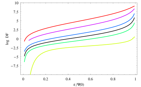
Figure 1: The normalized isotropic DF $\tilde{f}(\tilde{{\cal{E}}},n)$ as function of the normalized energy $\tilde{{\cal{E}}}/\tilde{\Psi}(0)$ for $n$ ranging from 1 to 9 in steps of 2 (from the bottom yellow to the top red curve) with the black line referring to the de Vaucouleurs ($n=4$) case. Note that, due to numerical reason, $\tilde{\Psi}(0)$ is actually $\tilde{\Psi}(10^{-4})$ without any significant loss of precision.

$$\tilde{\Psi}(\tilde{\eta})=\tilde{{\cal{E}}}\ .$$ (16)

Using Eqs.(3) and (10), it is only a matter of algebra to compute the different terms entering Eq.(15) for the PS model. We do not report here the full expressions for sake of shortness, but we stress that the second term identically vanishes, while the final DF is a function of the scaled energy $\tilde{{\cal{E}}}$ and the slope $n$ of the Sersic profile. Moreover, since putting together Eqs.(4) and (6) gives :

$$\rho_{0}=\Upsilon_{\star}j_{0}=\frac{M_{\star}}{4\pi R_{eff}^{3}}\frac{b_{n}^{n(3-p_{n})}}{n\Gamma[n(3-p_{n})]}\ ,$$ (17)

we can rewrite the isotropic DF for the PS model as :

$$f({\cal{E}})=\frac{\tilde{f}(\tilde{{\cal{E}}},n)}{G^{3/2}\Upsilon_{\star}^{1/2}j_{0}^{1/2}R_{eff}^{3}}=\frac{\lambda(n)\tilde{f}(\tilde{{\cal{E}}},n)}{G^{3/2}M_{\star}^{1/2}R_{eff}^{3/2}}$$ (18)

with $I_{0}=I(R=0)=I_{e}{\rm e}^{b_{n}}$ and :

$$\lambda(n)=\left\{\frac{n\Gamma[4\pi n(3-p_{n})]}{b_{n}^{n(3-p_{n})}}\right\}^{1/2}\ .$$ (19)

Fig. 1 shows the normalized DF $\tilde{f}(\tilde{{\cal{E}}},n)$ as function of $\tilde{{\cal{E}}}$ over the energy range $\tilde{\Psi}(\eta_{min})\leq\tilde{{\cal{E}}}\leq\tilde{\Psi}(\eta_{max})$ with $(\eta_{min},\eta_{max})=(10^{-4},10^{4})$. It is worth noting that the resulting DF is always positive that is to say the PS model is a physical one whatever the value of $n$ is.

4 The anisotropic DF

According to the model we are investigating, the PS density profile and DF describe the initial configuration of the baryons which will then originate the visible part of the galaxy. Let us now assume that a physical mechanism takes place injecting angular momentum into this initial configuration. Such an injection can be attributed, for instance, to the action of tidal torques between neighboring protogalaxies. As the protogalaxy collapses, it spins more and more rapidly thus acquiring angular momentum. As a further possibility, it is worth remembering that a merger of two disc galaxies also produces a spheroidal stellar system retaining angular momentum from the original rotating discs. Investigating the details of how angular momentum is injected in the initial PS - like configuration is outside our aims here, but we just recall these two possible scenarios to show that such a transfer of angular momentum is indeed possible. As a consequence, the phase space distribution of stars will be altered thus deviating from the isotropic DF we have considered above.

For spherically anisotropic systems, the DF may depend not only on the energy ${\cal{E}}$, but also on the total angular momentum $L$. In particular, we will focus our attention on the Osipkov - Merritt (OM) models [Osipkov 1979, Merritt 1985] where the DF reads :

$$f({\cal{E}},L)=f_{0}(Q)L^{2\alpha}$$ (20)

where the isotropic DF $f_{0}$ is evaluated in the lowered binding energy $Q={\cal{E}}-L^{2}/2r_{a}^{2}$. The slope parameter $\alpha$ and the anisotropy radius $r_{a}$ determine the velocity dispersion anisotropy profile given by :

$$\beta(r)=\frac{r^{2}-\alpha r_{a}^{2}}{r^{2}+r_{a}^{2}}\ .$$ (21)

For a positive $\alpha$, the anisotropy is tangential for $r^{2}<\alpha r_{a}^{2}$ to become then radial for $r^{2}/r_{a}^{2}>\alpha$. On the other hand, a negative $\alpha$ gives a model which is radially anisotropic everywhere whatever the value of $r_{a}$ is. Note that, for $\alpha=0$ and $r_{a}=1$, we obtain a model which is isotropic in the inner region and radially anisotropic in the outer ones.

The density profile corresponding to the anisotropic OM models may be computed as [Cudderford 1991] :

$$\rho(r) = \frac{(2\pi)^{3/2}(2r^{2})^{\alpha}}{(1+r^{2}/r_{a}^{2})^{\alpha+1}}\frac{\Gamma(\alpha+1)}{\Gamma(\alpha+3/2)}$$

$${\times} \int_{0}^{\Psi}{f_{0}(Q)(\Psi-Q)^{\alpha+1/2}dQ}\ .$$ (22)

Inserting Eq.(18) for the isotropic DF and changing variable from $Q$ to $\tilde{Q}=Q/4\pi G\rho_{0}R_{eff}^{2}$, we easily get :

$$\rho(\tilde{\Psi},\eta) = \frac{(2\pi)^{3/2}(2R_{eff}^{2})^{\alpha}\eta^{2\alpha}}{(1+\eta^{2}/\eta_{a}^{2})^{\alpha+1}}\frac{\Gamma(\alpha+1)}{\Gamma(\alpha+3/2)}$$

$${\times} \frac{(4\pi G\rho_{0}R_{eff}^{2})^{\alpha+3/2}}{G^{3/2}\rho_{0}^{1/2}R_{eff}^{3}}\int_{0}^{\tilde{\Psi}}{\tilde{f}(\tilde{Q},n)(\tilde{\Psi}-\tilde{Q})^{\alpha+1/2}d\tilde{Q}}$$

$$= \frac{2^{(6\alpha+9)/2}\pi^{\alpha+3}\Gamma(\alpha+1)}{\Gamma(\alpha+3/2)\tilde{\Psi}_{0}^{-(\alpha+3/2)}}\ {\times}\ G^{\alpha}\rho_{0}^{\alpha+1}R_{eff}^{4\alpha}$$

$${\times} \frac{\eta^{2\alpha}}{(1+\eta^{2}/\eta_{a}^{2})^{\alpha+1}}\int_{0}^{\psi}{\tilde{f}(q,n)(\psi-q)^{\alpha+1/2}dq}$$ (23)

where we have also introduced the more manageable variables $\psi=\tilde{\Psi}/\tilde{\Psi}_{0}$, $q=\tilde{Q}/\tilde{\Psi}_{0}$, with $\tilde{\Psi}_{0}=\tilde{\Psi}(\eta=0)$.

As an important step, we have to check that the right hand side of Eq.(23) has indeed the physical dimensions of a mass density. It is straightforward to verify that this is not the case because of the term $(G\rho_{0}R_{eff})^{\alpha}$. The origin of this discrepancy may be, however, easily understood noting that $G\rho_{0}R_{eff}^{4}$ has the same physical dimensions as $L^{2}$, i.e. the square modulus of the angular momentum. Actually, in Eq.(20), we have implicitly assumed that $L$ is dimensionless in order to follow the common practice. However, more correctly, we must introduce an (up to now) arbitrary normalization constant angular momentum $L_{0}$ to recover the correct result. Taking care of this and using Eq.(11) for $\tilde{\Psi}_{0}$, we therefore rewrite the mass density as :

$$\rho(\psi,\eta) = \frac{2^{(6\alpha+9)/2}\pi^{\alpha+3}\Gamma(\alpha+1)}{\Gamma(\alpha+3/2)}\left\{\frac{n\Gamma[n(2-p_{n})]}{b_{n}^{n(2-p_{n})}}\right\}^{\alpha+3/2}$$

$${\times} \left(\frac{L_{eff}}{L_{0}}\right)^{2\alpha}\ \frac{\rho_{0}\eta^{2\alpha}\hat{\rho}(\psi,n,\alpha)}{(1+\eta^{2}/\eta_{a}^{2})^{\alpha+1}}$$ (24)

having naively defined :

$$L_{eff}=\sqrt{G\rho_{0}R_{eff}^{4}}\ ,$$ (25)

$$\hat{\rho}(\psi,n,\alpha)=\int_{0}^{\psi}{\tilde{f}(q,n)(\psi-q)^{\alpha+1/2}dq}\ .$$ (26)

Eq.(24) gives $\rho$ as function of $\psi$ and $\eta$, while one is usually interested in $\rho$ as function of $\eta$ only. To this aim, we have to first solve the Poisson equation for the scaled dimensionless potential $\psi$. Starting from

$$\nabla^{2}\Psi=-4\pi G\rho\ ,$$

it is immediate to get :

$$\nabla^{2}\psi=\frac{1}{\eta^{2}}\frac{d}{d\eta}\left(\eta^{2}\frac{d\psi}{d\eta}\right)=-\frac{\rho}{\tilde{\Psi}_{0}\rho_{0}}\ ,$$

so that we have to solve the following differential equation :

Figure 2: The shape of the density profile of the OM - PS model. In the left panel, we set $\log{(L_{eff}/L_{0})}=0.0$ and $\alpha=0.15$ (short dashed), $0.50$ (solid), $0.75$ (long dashed), while in the right panel $\alpha=0.50$ and three values of $\log{(L_{eff}/L_{0})}$ are considered, namely $-1.0$ (short dashed), $0.0$ (solid), $1.0$ (long dashed). We arbitrarily set $n=4$ and $\eta_{a}=r_{a}/R_{eff}=0.01$ in both panels.

$$\nabla^{2}\psi = -\frac{2^{(6\alpha+9)/2}\pi^{\alpha+3}\Gamma(\alpha+1)}{\Gamma(\alpha+3/2)}\left\{\frac{n\Gamma[n(2-p_{n})]}{b_{n}^{n(2-p_{n})}}\right\}^{\alpha+1/2}$$

$${\times} \left(\frac{L_{eff}}{L_{0}}\right)^{2\alpha}\ \frac{\eta^{2\alpha}\hat{\rho}(\psi,n,\alpha)}{(1+\eta^{2}/\eta_{a}^{2})^{\alpha+1}}\ .$$ (27)

Needless to say, solving this equation analytically is not possible given its high nonlinearity because of the way $\psi$ enters in the determination of $\hat{\rho}(\psi,n,\alpha)$. However, a numerical solution is possible provided one sets the Sersic index $n$, the anisotropy parameters $(\alpha,\eta_{a})$, and the scaled characteristic angular momentum $L_{eff}/L_{0}$. Once such a solution for $\psi$ has been obtained, we can numerically invert the relation $\psi=\psi(\eta)$ to finally get $\rho=\rho(\eta)$. It is, however, worth stressing that, as a consequence of how $\psi(\eta)$ has been obtained, the mass density $\rho(\eta)$ will be parameterized by the quantities $(n,\alpha,\eta_{a},L_{eff}/L_{0})$ which are therefore the four parameters needed to assign the anisotropic OM - PS model.

It is interesting to look at the density profile of the OM - PS model. To this end, we show in Fig. 2 the normalized density $\rho_{s}=\eta^{2\alpha}/(1+\eta^{2}/\eta_{a}^{2})^{\alpha+1}\hat{\rho}(\eta)$ for models with $n=4$ arbitrarily setting $\eta_{a}=0.01$. As a general result, we note that an inner core developes when adding angular momentum to the orbit distribution. As left panel shows, the higher is $\alpha$, the more prominent is the core, i.e. $\rho_{s}\sim const$ for $\eta<\eta_{c}$ with $\eta_{c}$ an increasing function of $\alpha$. However, outside this inner region, the model resembles the original PS one so that it is likely that its projection still recovers the Sersic surface brightness profile with great precision everywhere but for $\eta<\eta_{c}$. Since $\eta_{c}$ is typically quite small $(\eta_{c}\sim 0.01)$, we can still use the value of $n$ retrieved from fitting the Sersic law to the observed photometry, which is what we will assume hereafter. Concerning the role of $L_{eff}/L_{0}$, right panel shows that it is mainly a scaling parameter shifting up the full profile as $L_{eff}/L_{0}$ becomes smaller. While changing $n$ leaves qualitatively unaltered the above results, the value adopted for $\eta_{a}$ plays a most significant role. Indeed, depending on the $(\alpha,L_{eff}/L_{0})$, should $\eta_{a}$ be larger than a critical value, $\rho_{s}(\eta)$ can also become an increasing function of $\eta$ in the very inner regions thus leading to an unphysical density profile. Investigating in detail what is the region of the 4D parameter space $(n,\alpha,\eta_{a},L_{eff}/L_{0})$ giving rise to physically meaningful OM - PS models is, however, outside our aims here. As a final remark, we warn the reader to not use Eq.(17) to replace $\rho_{0}$ with the total mass $M_{\star}$ in Eq.(25) since Eq.(17) only holds when $\rho(r)$ has the functional expression given by Eq.(3) which is not the case here. Nevertheless, one can still resort to Eq.(4) since this is an outcome of the requirement that the projected PS model matches the Sersic profile which is still approximately true for the OM - PS case (except in the very inner regions).

5 The size - mass relation

Notwithstanding the anisotropy in the velocity space, the spherical symmetry of the system makes it possible to compute the total mass as :

$$M_{\star}=4\pi\int_{0}^{\infty}{r^{2}\rho(r)dr}=4\pi R_{eff}^{3}\int_{0}^{\infty}{\eta^{2}\rho(\eta)d\eta}\ .$$

It is now only a matter of algebra to insert Eq.(23) into the above relation to get :

$$M_{\star} = \frac{2^{(6\alpha+13)/2}\pi^{\alpha+4}\Gamma(\alpha+1)}{\Gamma(\alpha+3/2)}\left\{\frac{{\rm e}^{b_{n}}b_{n}^{n(1-p_{n})}\Gamma(2n)}{\Gamma[n(3-p_{n})]}\right\}$$

$${\times} \left\{\frac{n\Gamma[n(2-p_{n})]}{b_{n}^{n(2-p_{n})}}\right\}^{\alpha+3/2}\left(\frac{L_{eff}}{L_{0}}\right)^{2\alpha}\Upsilon_{\star}I_{e}R_{eff}^{2}$$

$${\times} {\cal{I}}(n,\alpha,\eta_{a},L_{eff}/L_{0})\ ,$$ (28)

where we have used $\rho_{0}=\Upsilon_{\star}j_{0}$ with $j_{0}$ from Eq.(4) and defined :

$${\cal{I}}(n,\alpha,\eta_{a},L_{eff}/L_{0})=\int_{0}^{\infty}{\frac{\eta^{2\alpha+2}\hat{\rho}(\eta)}{(1+\eta^{2}/\eta_{a}^{2})^{\alpha+1}}d\eta}\ .$$ (29)

Note that, when $\alpha=0$, the density profile reduces to the original PS one and we get the usual result $M_{\star}\propto R_{eff}^{2}$, i.e. $\log{R_{eff}}\propto(1/2)\log{M_{\star}}$, as expected.

Let us now suppose that, for a fixed value of $n$, the mass integral (29) can be approximated as :

$$\log{{\cal{I}}} = a+b\alpha+c\log{{\cal{L}}_{eff}}+d\log{\eta_{a}}$$

$$+ e\alpha\log{{\cal{L}}_{eff}}+f\alpha\log{\eta_{a}}$$ (30)

with ${\cal{L}}_{eff}=L_{eff}/L_{0}$ and $(a,b,c,d,e,f)$ constant parameters to be determined. Inserting this ansätz into Eq.(28) gives :

$$M_{\star} = \frac{2^{(6\alpha+13)/2}\pi^{\alpha+4}\Gamma(\alpha+1)}{\Gamma(\alpha+3/2)}\left\{\frac{\rm{e}^{b_{n}}b_{n}^{n(1-p_{n})}\Gamma(2n)}{\Gamma[n(3-p_{n})]}\right\}$$

$$\times \left\{\frac{n\Gamma(2n)}{b_{n}^{n(2-p_{n})}}\right\}^{\alpha+3/2}\Upsilon_{\star}I_{e}R_{eff}^{2}$$

$$\times {\cal{A}}(\alpha)\ \eta_{a}^{d+f\alpha}\ {\cal{L}}_{eff}^{c+(e+2)\alpha}\ ,$$ (31)

with :

$${\cal{A}}(\alpha)=10^{a+b\alpha}\ .$$

Using Eqs.(4) and (25), it is trivial to show that :

$${\cal{L}}_{eff}^{c+(e+2)\alpha} = \left\{\frac{{\rm e}^{b_{n}}b_{n}^{n(1-p_{n})}\Gamma(2n)}{2\Gamma[n(3-p_{n})]}\right\}^{\frac{c+(e+2)\alpha}{2}}$$

$$\times \left(\frac{G\Upsilon_{\star}I_{e}}{L_{0}^{2}}\right)^{\frac{c+(e+2)\alpha}{2}}\ R_{eff}^{\frac{3[c+(e+2)\alpha]}{2}}\ .$$ (32)

Inserting this relation into Eq.(31) and using logarithmic units, it is then only a matter of algebra to finally get :

$$\log{R_{eff}}=\log{R_{10}}+\gamma\log{\left(\frac{M_{\star}}{2{\times}10^{10}\ h^{-1}\ {\rm M_{\odot}}}\right)}$$ (33)

with :

$$\gamma=\left[\frac{(3e+6)\alpha+(3c+4)}{2}\right]^{-1}\ ,$$ (34)

$$\log{R_{10}}=\gamma\log{(2{\times}10^{10}h^{-1}M_{\odot})}-\log{{\cal{N}}(\alpha)}\ ,$$ (35)

$${\cal{N}}(\alpha) = \frac{2^{(6\alpha+13)/2}\pi^{\alpha+4}\Gamma(\alpha+1)}{\Gamma(\alpha+3/2)}\left\{\frac{n\Gamma[n(2-p_{n})]}{b_{n}^{n(2-p_{n})}}\right\}^{\alpha+3/2}$$

$$\times \left\{\frac{{\rm e}^{b_{n}}b_{n}^{n(1-p_{n})}\Gamma(2n)}{\Gamma[n(3-p_{n})]}\right\}^{\frac{(e+2)\alpha+(c+2)}{2}}\Upsilon_{\star}I_{e}{\cal{A}}(\alpha)$$

$$\times \left(\frac{G\Upsilon_{\star}I_{e}}{2L_{0}^{2}}\right)^{\frac{(e+2)\alpha+c}{2}}\ \eta_{a}^{f\alpha+d}\ .$$ (36)

Should all the ETGs have the same values of the photometric parameters $(n,I_{e})$, the stellar $M/L$ ratio $\Upsilon_{\star}$ and the anisotropy parameters $(\alpha,\eta_{a})$, then their sizes and masses should turn out to be perfectly correlated as predicted by Eq.(33). Observationally, such a correlation is indeed found, but with an intrinsic scatter which may be obviously due to the scatter in the quantities entering the definitions of $\gamma$ and $R_{10}$. Assuming, however, as a first approximation that $n=4$ for all galaxies (i.e., all the ETGs follow the de Vaucouleurs surface brightness profile) and that $(\alpha,\eta_{a})$ do not change on a case - by - case basis, we can then estimate $\alpha$ and $L_{0}$ from the observed values of $\gamma$ and $R_{10}$ once the fitting coefficients $(a,b,c,d,e,f)$ have been determined. This latter task can be easily done by computing the mass integral over a grid in the $(\alpha,{\cal{L}}_{eff},\eta_{a})$ space for a fixed value of $n$. In particular, for $n=4$, we find :

$$(a,b,c,d,e,f)\simeq(-2.357,1.780,-0.017,0.223,-2.316,0.114)$$

fits very well the mass integral in Eq.(29) with a mean percentage residual $\langle\Delta{\cal{I}}/{\cal{I}}\rangle\simeq 0.1\%$ and $(\Delta{\cal{I}}/{\cal{I}})_{rms}\simeq 6\%$. With these values, the slope of the size - mass relation turns out to be :

$$\gamma\simeq(1.974-0.474\ \times\ \alpha)^{-1}$$

so that, setting $\gamma=0.56$ as observationally found by Shen et al. (2003) for ETGs with $M_{\star}>2{\times}10^{10}\ h^{-1}\ {\rm M_{\odot}}$, we finally get $\alpha\simeq 0.40$, i.e. the velocity anisotropy is tangential for $r/r_{a}<\sqrt{\alpha}\simeq 0.63$ and radial elsewhere. For lower mass systems, Shen et al. (2003) find $\gamma=0.14$ thus giving $\alpha=-10.2$. Such a large negative value should argue in favor of a fully radial anisotropy, but also imply a quite strong angular momentum term in the anisotropic DF which seems quite unusual. Moreover, we have computed the mass integral only for $\alpha>0$ so that our approximation for $\log{{\cal{I}}}$ should not be extrapolated to models with negative $\alpha$.

It is worth stressing, however, that the surface brightness profile of dwarf ellipticals is better fitted by Sersic profiles with $n=1$ rather than $n=4$ so that the above relation between $\alpha$ and $\gamma$ does not apply anymore. We have therefore recomputed the mass integral over the same grid, but setting now $n=1$. This gives us :

$$(a,b,c,d,e,f)\simeq(-1.641,0.644,-0.927,-0.463,-2.491,0.662)$$

thus giving :

$$\gamma\simeq(0.609-0.736\ \times\ \alpha)^{-1}\ .$$

Unfortunately, setting $\gamma=0.14$ and solving for $\alpha$, we get $\alpha\simeq-8.9$ so that we are unable to escape the same problems as with $n=4$. Moreover, our approximating expression (30) now works well only over a limited range in $({\cal{L}}_{eff},\eta_{a})$ with significantly worse residuals ($\langle\Delta{\cal{I}}/{\cal{I}}\rangle\simeq 6\%$, $(\Delta{\cal{I}}/{\cal{I}})_{rms}\simeq 14\%$). We therefore caution the reader to not overrate the validity of the $\gamma$ - $\alpha$ relation for $n=1$ Sersic models.

6 A dark size - mass relation

Although our main aim was to investigate the size - mass relation for the visible component of ETGs, it is worth stressing that the above procedure is quite general. As an interesting application, we consider dark haloes since it has been proposed [Merritt et al. 2006] that the PS model best approximates the density profile of dark haloes coming out from dark matter only simulations. Actually, the PS parameters change from one case to another so that a general rule could not be extracted. Nevertheless, the value of $n$ is not too dispersed so that we will repeat the above calculation setting $n$ to the average value $n=3.58$. As a result, we obtain for the slope $\gamma$ of the $R_{eff}$ - $M$ relation :

$$\gamma\simeq 1.915-0.263\times\alpha\ .$$

An important remark is in order here. Since we are now using the PS model for the dark halo, $R_{eff}$ and $M$ can no more be estimated unless one fits the model to kinematical (such as the velocity dispersion profile) or lensing (e.g., Einstein rings) data. As such, we cannot provide any estimate neither for $\alpha$ or $\gamma$. However, it is convenient to reparameterize the size - mass relation for haloes in terms of the concentration parameter and the virial mass. Without loss of precision, we can simply identify the halo virial mass with the PS total mass. In order to define a concentration for the PS halo, we first introduce the scale radius $r_{s}$ defined by the condition :

$$\frac{d\ln{\rho}}{d\ln{r}}=-2$$

in close analogy with the meaning of $r_{s}$ in the NFW model. Using Eq.(3), we easily get :

$$r_{s}=\left[\frac{n(2-p_{n})}{b_{n}}\right]^{n}R_{eff}\ .$$ (37)

The concentration $c_{PS}$ may be then defined as $c_{PS}=R_{vir}/r_{s}$, and, using $R_{vir}\propto M_{vir}^{1/3}$ and $R_{eff}\propto M_{vir}^{\gamma}$, we finally get :

$$c_{PS}\propto M_{vir}^{-\gamma_{DM}}$$

with :

$$\gamma_{DM}=\gamma-1/3\simeq\frac{1.085+0.263\times\alpha}{3(1.915-0.263\times\alpha)}\ .$$

For $0\leq\alpha\leq 1$, we get $0.19\leq\gamma_{DM}\leq 0.27$, so that the concentration is a mild decreasing function of the virial mass. Such a behavior is in agreement with the results of simulations, but a direct comparison is not possible because of the use of different halo models.

7 Conclusions

In the present paper, we studied the effect of injecting angular momentum in a Sersic isotropic profile. Our starting motivation was to investigate the role of angular momentum in explaining the discrepancy between FP projections (in our case, the $R_{eff}$ - $M_{\star}$ relation) and observations. Moreover, such a work can also shed light on the differences between dwarf and normal ellipticals as evidenced by the same FP projections.

Injecting angular momentum makes the velocity dispersion tensor anisotropic so that the DF has to be accordingly modified. The Osipkov - Merritt parameterization provides a valuable tool to infer the corresponding DF and hence the modified density profile. As a consequence, the size - mass relation turns out to be changed with respect to the isotropic case thus tilting the $\log{R_{eff}}$ - $\log{M_{\star}}$ relation with respect to the isotropic value. As we have shown, the slope $\gamma$ of the size - mass relation is an easy function of the anisotropy parameter $\alpha$. For massive ($M_{\star}\geq 2\times 10^{10}\ h^{-1}\ {\rm M_{\odot}}$ETGs, our model may be reconciled with the data provided the anisotropy profile is tangential in the inner regions (i.e., for $r/r_{a}<0.6$) to become then radial elsewhere. It is worth noting that, while $\alpha$ is the only parameter controlling the slope of the size - mass relation, all the three quantities $(\alpha,r_{a},L_{0})$ enter in determining the zeropoint of the correlation. As a consequence, while $\alpha$ can be determined by $\gamma$, we cannot infer a unique value for the anisotropy scale $r_{a}/R_{eff}$ unless we estimate somewhat the reference angular momentum $L_{0}$.

Actually, the unique way to break this degeneracy relies on fitting the velocity dispersion profile for a statistically meaningful sample of ETGs in order to determine, on a case - by - case basis, the value of $(\alpha,r_{a}/R_{eff})$. Such a test is also mandatory in order to check the validity of the assumed OM parameterization of the anisotropy profile. Moreover, the distribution of the $(\alpha,r_{a}/R_{eff})$ values can provide an estimate of the expected scatter in the $\log{R_{eff}}$ - $\log{M_{\star}}$ relation thus giving a further cross check of the model.

It is worth wondering whether our results can help in elucidating why dwarfs and giant ellipticals present surprising structural differences. Indeed, while dEs appear as the natural low luminosity counterpart of giant Es, they do not follow the same scaling relations as the latter ones. For instance, the $R_{eff}$ - $M_{\star}$ relation is rather shallow with a slope $\gamma=0.14$ significantly smaller than the one $(\gamma=0.56)$ of the high mass ellipticals. To this end, we first remember that, while both normal and dEs formed from the gravitational collapse of primordial density fluctuations, their structural and stellar population properties depend on the ability of the baryons in a given overdense region to cool and form stars. In particular, a feedback mechanism that transfers energy back to the interstellar medium is usually invoked to explain the dEs structure. For instance, models that invoke the cessation of star formation by supernova driven winds provide a plausible explanation for the variation of density (surface brightness) and metallicity (color) with luminosity (Larson 1974; Saito 1979; Vader 1986; Dekel & Silk 1986; Arimoto & Yoshii 1987). On the other hand, in Del Popolo (2002) and Del Popolo et al. (2005), it has been shown that a similar role may also be played by the acquisition of angular momentum. Indeed, the acquisition of a higher amount of angular momentum by a less dense region helps contrasting the gravitational collapse and hence prevents the cooling of baryons and the star formation.

Based on this latter model, we therefore expect thart injecting angular momentum in the dEs DF produces a decrease of mass infall towards the centre thus giving rise to a structure with lower central surface brightness. In order to qualitatively confirm this picture, it is worth remembering that dEs present roughly three different morphologies with most bright dwarfs $(M_{B}\leq-16)$ presenting a distinct luminosity spike in their centre (referred to as the nucleus). Lower luminosities dwarfs do not present such a nuclear region and may be divided in S0 - like and elliptical - like with this latter tipycally having a very low surface brightness. The different morphology with luminosity can be explained, in the previous scheme, as follows: bright dwarfs are born from higher density peaks, less subject to tidal torque, and as a consequence one expects that more mass freely fall to the centre giving rise to the central nucleus. Low surface brightness types are born from lower density peaks which suffer a larger tidal torque. This produce galaxies without a central nucleus, more extended and having low surface brightness. We have previously seen that in order to explain the $R_{eff}$ - $M_{\star}$ scaling law for dEs we need a negative value of $\alpha$ implying a large angular momentum term in the anisotropic DF, somehow in agreement with this qualitative picture. Moreover, the finding that very different values for $\alpha$ are needed in order to explain the reproduced the observed size - mass relation for dEs and normal Es confirms our notion that they have a very different dynamical origin.

While the outcome of this simplified investigation goes in the right direction, more work is needed in order to put these preliminary results on a firmer ground. As a first major improvement, one has to give off the hypothesis of spherical symmetry allowing for rotational flattening. This is particularly important since some evidences argue in favour of dEs being the final evolutionary state of tidal dwarfs galaxies (Gentile et al. 2007) thus originating from rotationally supported gas rich tidal arms. It is therefore worth investigating whether injecting angular momentum in the DF of a flattened PS model may allow us to still preserve our predicted $R_{eff}$ - $M_{\star}$ relation and, at the same time, solving the problem of the negative $\alpha$ needed to reproduce the observed slope. Should this be the case, we could have a strong evidence in favour of angular momentum playing the leading role in determining the structure of dwarf ellipticals.

References

- [Arimoto & Yoshii 1987] Arimoto, N., Yoshii Y., 1987, A&A, 173, 23
- [Baum 1990] Baum, W.A. 1990, ASP Conf. Ser. 10 : Evolution of the Universe of Galaxies, 10, 119
- [Barazza et al. 2002] Barazza, F., Binggeli, B., Jerjen, H., 2002, A&A, 391, 823
- [Bender et al. 1992] Bender, R., Burstein, D., Faber, S.M. 1992, ApJ, 399, 462
- [Bender & Nieto 1990] Bender, R., Nieto J.L. 1990, A&A, 239, 97
- [Bernardi et al. 2003a] Bernardi, M., Sheth, R.K., Annis, J., Burles, S., Eisenstein, D.J. et al. 2003a, AJ, 125, 1866
- [\citeauthoryearBernardi et al.2003b] Bernardi, M., Sheth, R.K., Annis, J., Burles, S., Eisenstein, D.J. et al. 2003b, AJ, 125, 1849
- [Binney & Tremaine 1987] Binney, J., Tremaine, S. 1987, Galactic dynamics, Princeton University Press, Princeton (USA)
- [Boselli et al. 2001] Boselli, A., Gavazzi, G., Donas, J., Scodeggio, M. 2001, AJ, 121, 753
- [Boylan - Kolchin et al. 2005] Boylan - Kolchin, M., Ma, C.-P., Quataert, E. 2005, MNRAS, 362, 184
- [Bower et al. 1992] Bower, R.G., Lucey, J.R., Ellis, R.S. 1992, MNRAS, 254, 601
- [Burstein et al. 1997] Burstein, D., Bender, R., Faber, S., Nolthenius, R. 1997, AJ, 114, 1365
- [Caon et al. 1993] Caon, N., Capaccioli, M., D’ Onofrio, M. 1993, MNRAS, 265, 1013
- [Capaccioli et al. 1992] Capaccioli, M., Caon, N., D’Onofrio, M. 1992, MNRAS, 259, 323
- [Cardone & Sereno 2005] Cardone, V.F., Sereno, M. 2005, A&A, 438, 545
- [Catelan & Theuns 1996a] Catelan, P., Theuns, T. 1996a, MNRAS 282, 436
- [Catelan & Theuns 1996b] Catelan, P., Theuns, T. 1996b, MNRAS 282, 455
- [Ciotti & Bertin 1999] Ciotti, L., Bertin, G. 1999, A&A, 352, 477
- [Conselice et al. 2003] Conselice, C., O’Neil, K., Gallagher, J., Wyse, R. 2003, ApJ, 591, 167
- [Cudderford 1991] Cudderford, P. 1991, MNRAS, 253, 414
- [Dabringhausen el al. 2008] Dabringhausen, J., Hilker, M., Kroupa, P. 2008, MNRAS, 386, 864
- [Dekel & Silk 1986] Dekel, A., Silk, J. 1986, ApJ 303, 39
- [Del Popolo el al. 2005] Del Popolo, A., Hiotelis, N., Peńarrubia, J. 2005, ApJ 628, 76
- [Del Popolo 2002] Del Popolo, A. 2002, MNRAS, 336, 81
- [De Lucia et al. 2006] De Lucia, G., Springel, V., White, S.D.M., Croton, D., Kauffmann, G. 2006, MNRAS, 366, 499
- [de Vaucouleurs 1948] de Vaucouleurs, G. 1948, Ann. d’ Astroph., 11, 247
- [Dressler et al. 1987] Dressler, A., Lynden - Bell, D., Burstein, D., Davies, R.L., Faber, S.M., Terlevich, R.J., Wegner, G. 1987, ApJ, 313, 42
- [Djorgovski & Davis 1987] Djorgovski, S., Davis, M. 1987, ApJ, 313, 59
- [Eisenstein & Loeb 1995] Eisenstein, D.J., Loeb, A. 1995, ApJ 439, 520
- [Faber & Jackson 1976] Faber, S.M., Jackson, R.E. 1976, ApJ, 204, 668
- [Ferguson & Binggeli 1994] Ferguson, H., Binggeli, B. 1994, ARA&A, 6, 67
- [Gavazzi et al. 1996] Gavazzi, G., Pierini, D., Boselli, A. 1996, A&A, 312, 397
- [Gentile et al. 2007] Gentile, G., Famaey, B., Combes, F., Kroupa, P., Zhao, H.S., Tiret, O. 2007, A&A 472, L25
- [Gerhard et al. 2001] Gerhard, O., Kronawitter, A., Saglia, R.P., Bender, R. 2001, AJ, 121, 1936
- [Graham & Colless 1997] Graham, A.W., Colless, M. 1997, MNRAS, 287, 221
- [Graham & Guzman 2003] Graham, A., Guzman, R. 2003, AJ, 125, 2936
- [Graham & Driver 2005] Graham, A.W., Driver, S.P. 2005, PASA, 22, 118
- [Haines et al. 2007] Haines, C., Gargiulo, A., La Barbera, F., Mercurio, A., Merluzzi, P., Busarello, G. 2007, MNRAS, 381, 7
- [Held et al. 1990] Held E.V., Mould J., de Zeeuw T. 1990, AJ 100, 415
- [Hoffman 1986a] Hoffman, Y. 1986a, ApJ 308, 493
- [Hoffman 1986b] Hoffman, Y. 1986b, ApJ 301, 65
- [Hoyle 1949] Hoyle, F. 1949, in IAU and International Union of Theorethical and Applied Mechanics Symposium, p. 195
- [Jorgensen et al. 1996] Jorgensen, I., Franx, M., Kjaergaard, P. 1996, MNRAS, 280, 167
- [Kauffmann et al. 2003] Kauffmann, G., Heckman, T.M., White, S.D.M., Charlot, S., Tremonti, C., Brinchmann, J. et al. 2003, MNRAS, 341, 33
- [Keeton 2001] Keeton, C.R. 2001, ApJ, 561, 46
- [Klypin et al. 2003] Klypin, A., Zhao H.S., Somerville, R.S. 2002, ApJ 573, 597
- [Kormendy 1977] Kormendy, J. 1977, ApJ, 218, 333
- [Kormendy 1985] Kormendy, J., 1985, ApJ, 432, L63
- [Larson 1974] Larson, R.B. 1974, MNRAS 169, 229
- [Lisker et al. 2006a] Lisker, T., Grebel, E., Binggeli, B. 2006a, AJ, 132, 497
- [Lisker et al. 2006b] Lisker, T., Glatt, K., Westera, P., Grebel, E. 2006b, AJ, 132, 2432
- [Lisker et al. 2007] Lisker, T., Grebel, E., Binggeli, B., Glatt, K. 2007, ApJ, 660, 1186
- [Lisker et al. 2008] Lisker, T., Grebel, E., Binggeli, B. 2008, AJ, 135, 380
- [Lisker & Han 2008] Lisker, T., Han, Z. 2008, ApJ, 680, 1042
- [Lokas & Mamon 2001] Lokas, E.L., Mamon, G. 2001, MNRAS, 321, 155
- [Márquez et al. 2001] Márquez, I., Lima Neto, G.B., Capelato, H., Durret, F., Lanzoni, B., Gerbal, D. 2001, A&A, 379, 767
- [Mastropietro et al. 2008] Mastropietro, C., Moore, B., Mayer, L., Debattista, V., Piffaretti, R., Stadel, J. 2005, MNRAS, 364, 607
- [Mayer et al. 2006] Mayer, L., Mastropietro, C., Wadsley, J., Stadel, J., Moore, B. 2006, MNRAS, 369, 1021
- [Mazure & Capelato 2002] Mazure, A., Capelato, H.V. 2002, A&A, 383, 384
- [Merritt 1985] Merritt, D. 1985, AJ, 90, 1027
- [Merritt et al. 2006] Merritt, D., Graham, A.W., Moore, B., Diemand, J., Terzic, B. 2006, AJ, 132, 2685
- [Michielsen et al. 2006] Michielsen, D., Boselli, A., Conselice, C., Toloba, E., Wiley, E.M. et al. 2008, MNRAS, 385, 1374
- [Mo et al. 1998] Mo H.J., Mao, S., White S.D.M. 1998, MNRAS 295, 319
- [Moore et al. 1998] Moore, B., Lake, G., Katz, N. 1998 ApJ 495, 139
- [Osipkov 1979] Osipkov, L.P. 1979, Soviet Astron. Lett., 5, 42
- [Padmanabhan et al. 2004] Padmanabhan, N., Seljak, U., Strauss, M.A., Blanton, M.R., Kauffmann, G. et al. 2004, New Ast., 9, 329
- [Pahre et al. 1998] Pahre M.A., de Carvalho, R.R., Djorgovski S.G. 1998, AJ, 116, 1591
- [Peebles 1969] Peebles, P.J.E. 1969, ApJ 155, 393
- [Penny & Conselice 2008] Penny, S., Conselice, C. 2008, MNRAS, 383, 247
- [Prugniel & Simien 1997] Prugniel, Ph., Simien, F. 1997, A&A, 321, 111
- [Saito 1979] Saito, M. 1979, PASJ 31, 193
- [Sersic 1968] Sersic, J.L. 1968, Atlas de Galaxies Australes, Observatorio Astronomico de Cordoba
- [Shen et al. 2003] Shen, S., Mo, H.J., White, S.D.M., Blanton, M.R., Kauffmann, G., Voges, W., Brinkmann, J., Csabai, I. 2003, MNRAS, 343, 978
- [Smith et al. 2008] Smith, R.J., Marzke, R.O., Hornschemeier, A.E., Bridges, T.J., Hudson, M.J. et al. 2008, MNRAS, 386, L96
- [Treu & Koopmans 2002] Treu, T., Koopmans L.V.E. 2002, ApJ 575, 87
- [Trujillo et al. 2004] Trujillo, I., Burkert, A., Bell, E.F. 2004, ApJ, 600, L39
- [Tully & Fisher 1977] Tully, B., Fisher, J. 1977, A&A, 54, 661
- [Tully et al. 1982] Tully, B., Mould, J., Aaronson, M. 1982, ApJ, 257, 527
- [Vader 1986] Vader, J.P. 1986, ApJ, 305, 669
- [Van Zee et al. 2004] Van Zee, L., Skillman, E., Haynes, M. 2004, AJ, 128, 121
- [Visvanathan & Sandage 1977] Visvanathan, N., Sandage, A. 1977, ApJ, 216, 214