Accuracy of direct gradient sensing by single cells

Abstract

Many types of cells are able to accurately sense shallow gradients of chemicals across their diameters, allowing the cells to move towards or away from chemical sources. This chemotactic ability relies on the remarkable capacity of cells to infer gradients from particles randomly arriving at cell-surface receptors by diffusion. Whereas the physical limits of concentration sensing by cells have been explored, there is no theory for the physical limits of gradient sensing. Here, we derive such a theory, using as models a perfectly absorbing sphere and a perfectly monitoring sphere, which, respectively, infer gradients from the absorbed surface particle density or the positions of freely diffusing particles inside a spherical volume. We find that the perfectly absorbing sphere is superior to the perfectly monitoring sphere, both for concentration and gradient sensing, since previously observed particles are never remeasured. The superiority of the absorbing sphere helps explain the presence at the surfaces of cells of signal degrading enzymes, such as PDE for cAMP in Dictyostelium discoideum (Dicty) and BAR1 for mating factor $\alpha$ in Saccharomyces cerevisiae (budding yeast). Quantitatively, our theory compares favorably to recent measurements of Dicty moving up a cAMP gradient, suggesting these cells operate near the physical limits of gradient detection.

Cells are able to sense gradients of chemical concentration with extremely high sensitivity. This is done either directly, by measuring spatial gradients across the cell diameter, or indirectly, by temporally sensing gradients while moving. In temporal sensing, a cell modifies its swimming behavior according to whether a chemical concentration is rising or falling in time berg99 . This mode of sensing is typical of small, fast moving bacteria such as Escherichia coli, which can respond to changes in concentration as low as 3.2 nM of the attractant aspartate manson03 . In contrast, direct spatial sensing is prevalent among larger, single-celled eukaryotic organisms such as the slime mold Dictyostelium discoideum (Dicty) and the yeast Saccharomyces cerevisiae arkowitz99 ; manahan04 . Dicty cells are able to sense a concentration difference of only 1-5% across the cell mato75 , corresponding to a difference in receptor occupancy between front and back of only 5 receptors haastert07 . Spatial sensing is also performed with high accuracy by cells of the immune system including neutrophils and lymphocytes zigmond77 , as well as by growing synaptic cells and tumor cells. While there has been great progress in understanding the limits of concentration sensing and signaling in bacteria such as E. coli berg77 ; bray98 ; bialek05 ; mello05 ; keymer06 ; endres06 , very little is know about the theoretical limits of direct gradient sensing by eukaryotic cells.

In a recent set of experiments, van Haastert and Postma haastert07 measured the Chemotactic Index of Dicty cells in a cAMP gradient (Fig. 1, symbols). Chemotactic Index is defined as the distance moved in the direction of the cAMP gradient divided by the total distance moved. To obtain the data in Fig. 1, van Haastert and Postma used a pipette containing different concentrations of cAMP. Diffusion of cAMP out of the pipette established a steady-state cAMP gradient, with magnitude a function of distance from the pipette. Chemotaxis was observed for cells as far as 700 $\mu$m from a pipette filled with $10^{-4}$ M cAMP, corresponding to a mean concentration of 7 nM and a gradient of only 0.01 nM/$\mu$m. This remarkable chemotactic ability raises the question – how closely does gradient sensing by Dicty cells compare with the fundamental limits on gradient sensing set by diffusion?

Here we derive the fundamental limits of gradient sensing using two models for cells: a perfectly absorbing sphere and a perfectly monitoring sphere. Within the theory, gradients are estimated by comparing the discrete positions of particles, either absorbed on the surface of the sphere or measured inside the spherical volume, with the expected continuous distribution originating from a particular gradient. We find that a perfectly absorbing sphere is superior to a perfectly monitoring sphere for sensing both concentrations and gradients (Table I), since previously observed particles are never remeasured. Quantitatively, our theory (Fig. 1, solid curves) compares favorably with recent measurements of Dicty cells migrating to a cAMP-filled pipette haastert07 , suggesting that chemotactic ability of Dicty approaches the fundamental limits set by diffusion.

I Limits of Concentration Sensing

In this section, we consider the limits of concentration sensing set by particle diffusion. Consider as a measurement device a spherical cell of radius $a$ that can measure the local concentration of a certain dissolved chemical. Such an idealized device may make measurements following two different strategies: (1) The device can either act as a perfectly absorbing sphere and record the number of absorbed particles on its surface or (2) act as a perfectly monitoring sphere and count the number of particles inside its volume. In either case, from the number of particles, an estimate of the chemical concentration can be obtained. However, these estimates have an intrinsic uncertainty due to the randomness of particle diffusion.

Perfectly Absorbing Sphere. For the perfectly absorbing sphere the uncertainty in measuring a background chemical concentration $c$ is straightforward to derive. At steady state, the average particle current impinging on the sphere is $J=4\pi Dac$, where $D$ is the chemical diffusion constant. The average number of particles absorbed in time $T$ is $N=4\pi DacT$. Since the particles are independent, $N$ is Poisson distributed, i.e. $\langle(\delta N)^{2}\rangle=\langle N\rangle$. Therefore, the perfectly absorbing sphere has a concentration-measurement uncertainty of

$$\frac{\langle(\delta c)^{2}\rangle}{c^{2}}=\frac{\langle(\delta N)^{2}\rangle}{\langle N\rangle^{2}}=\frac{1}{4\pi DacT}.$$ (1)

Perfectly Monitoring Sphere. The perfectly monitoring sphere was introduced by Berg and Purcell berg77 as a parameter-free model for a cell that ”perfectly” binds and releases all ligands that contact its surface. To quantify the time a diffusing particle spends in the cell’s vicinity and is therefore capable of being measured, Berg and Purcell treated the cell as a permeable sphere that infers the particle concentration by counting the number of particles $N$ inside its volume, and improves accuracy by averaging over several statistically independent measurements. A simple estimate for the resulting uncertainty in concentration can be obtained as follows: the number $N$ is Poisson distributed and the cell counts appoximately $N=a^{3}c$ particles in its volume at any time. During a time $T$, the cell can make $N_{\text{meas}}=T/(a^{2}/D)$ independent measurements, where $a^{2}/D$ is the typical turnover time for particles inside the sphere, leading to

$$\frac{\langle(\delta c)^{2}\rangle}{c^{2}}=\frac{\langle(\delta N)^{2}\rangle}{N^{2}}=\frac{1}{N_{\text{meas}}N}\approx\frac{1}{DacT}.$$ (2)

Berg and Purcell berg77 derived the exact concentration-measurement uncertainty for a perfectly monitoring sphere (“perfect instrument”) from the time correlations of particles inside the sphere, and obtained

$$\frac{\langle(\delta c)^{2}\rangle}{c^{2}}=\frac{3}{5\pi DacT},$$ (3)

which is identical to the estimate in Eq. 2 up to a numerical prefactor.

However, notice that the concentration-measurement uncertainty of the perfectly absorbing sphere is actually smaller than that of a perfectly monitoring sphere of the same size, because the perfectly absorbing sphere removes particles from the environment, and hence does not measure the same particle more than once.

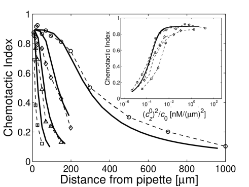
Figure 1: Comparison between the Chemotactic Index determined by experiment (symbols and dashed lines) and our theory (solid curves). Chemotactic Index is defined as the distance moved by a cell in the direction of a gradient divided by the total distance moved. Experimental data was obtained by van Haastert and Postma haastert07 from Dictyostelium discoideum cells migrating toward pipettes containing four different cAMP concentrations, 0.1 $\mu$M (squares), 1 $\mu$M (triangles), 10 $\mu$M (diamonds), 100 $\mu$M (circles). The theoretical curves were obtained for a perfectly absorbing sphere using a single fitting parameter $Da^{3}T=1.2\cdot 10^{5}\ \mu{\rm m}^{5}$, corresponding to, e.g., a cAMP diffusion constant of $D=300\ \mu{\rm m}^{2}/{\rm s}$, a cell radius of $a=5\ \mu{\rm m}$, and an averaging time $T=3.2\ {\rm s}$, using the gradient profiles from Ref. haastert07 and the Chemotactic Index from Eq. 21. Experimentally, the Chemotactic Index only reaches approximately 0.9 at zero distance, so we rescale our theory curves by 0.9. Inset: Chemotactic Index as a function of $(c_{z}^{0})^{2}/c_{0}$ in units of $n\text{M}/(\mu\text{m})^{2}$, where $c_{z}^{0}$ and $c_{0}$ are the gradient and concentration, respectively.

Figure 2: Idealized models for gradient sensing by a cell. The gradient points along the $z$-axis, which is shown horizontally. (a) Continuum model for a perfectly absorbing sphere. The mean particle current density $j(\theta)$ impinging on the sphere has axial symmetry; $\theta$ measures the angle with respect to the $z$-axis. At steady-state, the particle concentration $c$ is zero immediately outside the perfectly absorbing sphere, as shown schematically by the red curve superposed on the dotted background gradient. (b) Discrete particle model for the perfectly absorbing sphere. From the number and positions of particles absorbed during time $T$, the background particle concentration and gradient can be estimated. (c) Perfectly monitoring sphere. Particles diffuse in and out of the sphere without resistance. By monitoring, for a time $T$, the number and positions of particles inside the sphere, the background concentration and gradient can be estimated.

II Limits of Gradient Sensing

Now consider the perfectly absorbing sphere and the perfectly monitoring sphere as devices for measuring the local gradient of a certain dissolved chemical. In both cases, measurements of discrete particles can be compared with the expected continuous distribution of particles originating from a particular gradient (Fig. 2a), and hence, the gradient can be estimated. Here, we present in brief a theoretical derivation of the intrinsic uncertainty of gradient sensing (for details see supporting information). We find that the intrinsic uncertainty is independent of the actual gradient present, and is always much smaller (by a factor of 7/60 $\simeq$ 12%) for the perfectly absorbing sphere.

Perfectly Absorbing Sphere. The average particle current density $\vec{j}=-D\vec{\nabla}c$ impinging on the surface of a perfectly absorbing sphere of radius $a$ at steady state follows from the diffusion equation, $\nabla^{2}c=0$, and is given in polar coordinates by

$$j(\theta,\phi)=\frac{Dc_{0}}{a}+3D\vec{c}_{r}\cdot\vec{e}(\theta,\phi),$$ (4)

where $c_{0}$ is a constant background concentration, $\vec{c}_{r}$ is the background gradient, and $\vec{e}(\theta,\phi)=(\cos\phi\sin\theta,\sin\phi\sin\theta,\cos\theta)$ is a unit vector normal to the surface of the sphere (see Fig. 2a). To best estimate the chemical gradient from an observed discrete density of particles absorbed at the surface of the sphere during time $T$ (Fig. 2b), requires fitting the observed density $\sigma_{T}^{\text{obs}}=\sum_{i=1}^{N}\delta(\vec{r}-\vec{r}_{i})$, where $N$ is the total number of absorbed particles, to the expected density $j(\theta,\phi)\,T$ from Eq. 4. Since the estimates of the components of the gradient in the $x,y$, and $z$ directions are independent, without loss of generality, we consider only the gradient estimate in the $z$-direction, i.e. $c_{z}=\partial c/\partial z$, and later generalize to an arbitrary gradient. From the best fit, the estimate for the gradient in the $z$-direction after absorption of particles for a time $T$ is given by

$$c_{z}=\frac{\int\sigma_{T}^{\text{obs}}\cos\theta\,dA}{4\pi Da^{2}T}=\frac{\sum_{i=1}^{N}\cos\theta_{i}}{4\pi Da^{2}T},$$ (5)

where $\theta_{i}$ is the polar angle of the $i$th absorbed particle. We are interested in the uncertainty (accuracy) of the gradient measurement, which is given by the variance

$$\langle(\delta c_{z})^{2}\rangle=\langle c_{z}^{2}\rangle-\langle c_{z}\rangle^{2}$$

$$= \frac{\langle\sum_{i=1}^{N}\cos^{2}\theta_{i}\rangle+\langle\sum_{i=1}^{N}\sum_{i\neq j}^{N}\cos\theta_{i}\cos\theta_{j}\rangle}{(4\pi Da^{2}T)^{2}}$$

$$\qquad-\frac{\langle\sum_{i=1}^{N}\cos\theta_{i}\rangle^{2}}{(4\pi Da^{2}T)^{2}}$$

$$= \frac{\langle\sum_{i=1}^{N}\cos^{2}\theta_{i}\rangle}{(4\pi Da^{2}T)^{2}}=\frac{\langle N\rangle\langle\cos^{2}\theta\rangle}{(4\pi Da^{2}T)^{2}}=\frac{c_{0}}{12\pi Da^{3}T}.$$

The derivation of Eq. II made use of the independence of the particles to factorize the expectation value as $\langle\sum_{i=1}^{N}\sum_{i\neq j}^{N}\cos\theta_{i}\cos\theta_{j}\rangle=\langle N(N-1)\rangle\langle\cos\theta\rangle^{2}=\langle N\rangle^{2}\langle\cos\theta\rangle^{2}$, since the number of absorbed particles $N$ is Poisson distributed. We also used $\langle N\rangle=4\pi Dac_{0}T$, as well as $\langle\cos^{2}\theta\rangle=1/3$. (The relation $\langle\cos^{2}\theta_{i}\rangle=\langle\cos^{2}\theta\rangle$ for absorbed particles holds even in the presence of a true gradient in the $z$ direction since the gradient-weighted contribution $~{}\langle\cos^{3}\theta\rangle$ is zero.)

In three dimensions, the total uncertainty of the gradient, normalized by $c_{0}/a$, is given by

$$\frac{\langle(\delta c_{\vec{r}})^{2}\rangle}{(c_{0}/a)^{2}}=\frac{3\langle(\delta c_{z})^{2}\rangle}{(c_{0}/a)^{2}}=\frac{1}{4\pi Dac_{0}T},$$ (7)

with the factor of 3 arising because each component of the gradient contributes independently to the total uncertainty. This result for the uncertainty in gradient sensing is independent of the magnitude of the actual gradient present, including the case when no actual gradient is present. Curiously, the result is numerically identical to the concentration-measurement uncertainty (Eq. 1).

Perfectly Monitoring Sphere.
Here, we extend Berg and Purcell’s analysis of the perfectly monitoring sphere (“perfect instrument”) to include gradient sensing. Specifically, we assume that the monitoring sphere measures not only the number but also the positions of all particles in its volume (Fig. 2c). The best estimate of the gradient is obtained by fitting a concentration gradient with a $c=c_{0}+\vec{c}_{r}\cdot\vec{r}$ to the observed time-averaged number density $\frac{1}{T}\int\!dt\rho_{\text{obs}}(t)=\frac{1}{T}\int\!dt\sum_{i=1}^{N}\delta(\vec{r}-\vec{r}_{i}(t))$, obtained by measuring the exact positions of all the particles inside the volume of the sphere for a time $T$. As above we focus on one component of the gradient, namely the gradient in the $z$-direction $c_{z}$, and obtain as a best estimate

$$c_{z}=\frac{\frac{1}{T}\int\!dt\int\!dVz\,\rho_{\text{obs}}(t)}{\int\!dVz^{2}},$$ (8)

where the integral $\int\!\!dV$ is over the volume of the sphere. We are interested in the variance of this estimated gradient

$$\langle(\delta c_{z})^{2}\rangle = \langle c_{z}^{2}\rangle-\langle c_{z}\rangle^{2}$$

$$= \left(\frac{15}{4\pi a^{5}}\right)^{2}\left[\langle m_{z,T}^{2}\rangle-\langle m_{z,T}\rangle^{2}\right],$$

where we have used $\int\!\!dV\!\!z^{2}=4\pi a^{5}/15$ and have defined

$$m_{z,T}=\frac{1}{T}\int\!dt\int dVz\rho_{\text{obs}}(t),$$ (10)

namely $m_{z,T}$ is the time-averaged total $z$-coordinate of particles inside the sphere. The expectation values in Eq. II are therefore given by

$$\langle m_{z,T}^{2}\rangle = \frac{1}{T^{2}}\left\langle\left(\int\!dt\int\!dVz\rho_{\text{obs}}(t)\right)^{2}\right\rangle$$

$$= \frac{1}{T^{2}}\int_{0}^{T}\!dt\int_{0}^{T}\!dt^{\prime}\langle m_{z}(t)m_{z}(t^{\prime})\rangle,$$

$$\langle m_{z,T}\rangle = \frac{1}{T}\left\langle\left(\int\!dt\int\!dVz\rho_{\text{obs}}(t)\right)\right\rangle$$

$$= \frac{1}{T}\int_{0}^{T}\!dt\langle m_{z}(t)\rangle,$$

where the quantity $m_{z}(t)$ is the total of the $z$-coordinates of all the particles inside the sphere at time $t$. To calculate $m_{z}(t)$, we consider the sphere embedded inside a much larger volume containing a total of $M$ particles. Then, $m_{z}(t)=\sum_{i=1}^{M}z_{i}(t)$, where $z_{i}$ is the z-coordinate of particle $i$ if this particle is inside the sphere and is zero otherwise. On average there will be $\langle N\rangle=\frac{4}{3}\pi a^{3}c_{0}$ particles inside the sphere at any time $t$. The auto-correlation function $\langle m_{z}(t)m_{z}(t^{\prime})\rangle$ of particles inside the sphere at time $t$ and time $t^{\prime}$ can consequently be calculated as

$$\langle m_{z}(t)m_{z}(t^{\prime})\rangle = \langle\sum_{i=1}^{M}\sum_{j=1}^{M}z_{i}(t)z_{j}(t^{\prime})\rangle$$

$$= \frac{4}{3}\pi a^{3}c_{0}\,u(t-t^{\prime})+\langle m_{z}(t)\rangle^{2},$$

where we have defined $u(t-t^{\prime})=\langle z(t)z(t^{\prime})\rangle$ for a single particle. Substituting Eqs. II and II into Eq. II results in

$$\langle(\delta c_{z})^{2}\rangle=\frac{75c_{0}}{4\pi a^{7}T^{2}}\int_{0}^{T}\!dt\int_{0}^{T}\!dt^{\prime}u_{0}(t-t^{\prime}).$$ (13)

By defining a correlation time $\tau_{z}=(1/a^{2})\int_{0}^{\infty}\!d\tau u(\tau)$ for the coordinate $z(t)$, the double time integral in Eq. 13 can be simplified, provided the time $T$ is much larger than $\tau_{z}$. Using time-reversal symmetry $u(\tau)=u(-\tau)$ for equilibrium diffusion (assuming small gradients), the variance simplifies to

$$\langle(\delta c_{z})^{2}\rangle=\frac{75c_{0}\tau_{z}}{2\pi a^{5}T}.$$ (14)

The remaining task is to calculate $\tau_{z}$, the probability that a particle with coordinate $z$ inside the sphere at time $t=0$ is still (or again) inside the sphere at a later time $\tau$. We first consider the case in which the background chemical concentration is uniform, and later consider the presence of an actual gradient. Based on the solution of the diffusion equation in three dimensions, if a unit amount of chemical is released at point $\vec{r}\,^{\prime}$, the concentration at point $\vec{r}$ at a later time $\tau$ is given by

$$f(|\vec{r}-\vec{r}\,^{\prime}|,\tau)=\frac{\exp\left(-\frac{|\vec{r}-\vec{r}\,^{\prime}|^{2}}{4D\tau}\right)}{(4\pi D\tau)^{\frac{3}{2}}}.$$ (15)

Using the result for the time integral from Ref. berg77 ,

$$\int_{0}^{\infty}\!d\tau\,f(|\vec{r}-\vec{r}\,^{\prime}|,\tau)=\frac{1}{4\pi D|\vec{r}-\vec{r}\,^{\prime}|},$$ (16)

the correlation time $\tau_{z}$ can be expressed as a volume integral over the sphere (the initial coordinate $\vec{r}\,^{\prime}$ is uniform in the sphere because we assume a uniform background chemical concentration)

$$\tau_{z} = \frac{1}{\frac{4}{3}\pi a^{5}}\int_{0}^{\infty}\!d\tau\int\!dV\,z\int\!dV^{\prime}\,z\,^{\prime}f(|\vec{r}-\vec{r}\,^{\prime}|,\tau)$$

$$= \frac{3}{16\pi^{2}Da^{5}}\int\!dV\,z\int\!dV^{\prime}\frac{z\,^{\prime}}{|\vec{r}-\vec{r}\,^{\prime}|}$$

$$= \frac{3}{16\pi^{2}Da^{5}}\int\!dV\,z\,\psi(r,\theta),$$

where $r=|\vec{r}|$. The function

$$\psi(r,\theta)=\int\!dV^{\prime}\frac{z\,^{\prime}}{|\vec{r}-\vec{r}\,^{\prime}|}=\int\!dV^{\prime}\frac{r\,^{\prime}\cos\theta^{\prime}}{|\vec{r}-\vec{r}\,^{\prime}|}$$ (18)

is analogous to the potential of a charge density in electrostatics, specifically the charge density $\rho(z\,^{\prime})=z^{\prime}=\rho(r\,^{\prime},\theta^{\prime})=r^{\prime}\cos\theta^{\prime}$ for $r^{\prime}\leq a$ and $\rho(r\,^{\prime})=0$ for $r^{\prime}>a$. To solve the final integral in Eq. II, we perform a multipole expansion of $\psi(r,\theta)$ in terms of Legendre polynomials $P_{l}(\cos\theta)$, exploiting the rotational symmetry of $\psi(r,\theta)$ about the $z$ axis jackson , leading to

$$\tau_{z}=\frac{2a^{2}}{105D}.$$ (19)

Now consider the contribution from an additional gradient with zero mean over the volume of the sphere. We need to perform the integrals over a non-uniform distribution in Eq. II. Since a gradient along the $z$-axis contributes a factor $\cos\theta$, which leads to the vanishing integral $\int_{0}^{\pi}\sin\theta\cos^{3}\theta d\theta=0$, we conclude that only the constant background contributes to the uncertainty in the gradient measurement. Therefore, Eq. 19 for $\tau_{z}$ remains true even when an actual gradient is present.

The result for $\tau_{z}$ in Eq. 19 can be used in Eq. 14 to obtain the normalized uncertainty of gradient measurement by the perfectly monitoring sphere

$$\frac{\langle(\delta c_{\vec{r}})^{2}\rangle}{(c_{0}/a)^{2}}=\frac{3\langle(\delta c_{z})^{2}\rangle}{(c_{0}/a)^{2}}=\frac{15}{7\pi Dac_{0}T},$$ (20)

where all three components of the gradient contribute independently. Hence, the perfectly monitoring sphere is not only inferior to the perfectly absorbing sphere for concentration sensing by a factor of $12/5$ in variance (cf. Eqs. 1 and 3), but is also inferior by an even larger factor of $60/7$ for gradient sensing (cf. Eq. 7).

Measurement uncertainty	Perfect absorber	Perfect monitor	Ratio absorber/monitor
Concentration: $\frac{\langle(\delta c)^{2}\rangle}{c_{0}^{2}}$	$\frac{1}{4\pi Dac_{0}T}$ berg77	$\frac{3}{5\pi Dac_{0}T}$	$\frac{12}{5}$$=2.4$
Gradient: $\frac{\langle(\delta c_{\vec{r}})^{2}\rangle}{(c_{0}/a)^{2}}$	$\frac{1}{4\pi Dac_{0}T}$	$\frac{15}{7\pi Dac_{0}T}$	$\frac{60}{7}$$\approx 8.6$

Table 1: Uncertainties in measured concentration and concentration gradient for two idealized cell models: a perfectly absorbing sphere (second column) and a perfectly monitoring sphere (third column). Also provided is the ratio of the uncertainties of the absorber and monitor. Parameters: diffusion constant $D$, radius of sphere $a$, averaging time $T$, and average chemical concentration $c_{0}$.

III Comparison with Experiment

Van Haastert and Postma haastert07 recently measured the Chemotactic Index of Dicty cells in a cAMP gradient haastert07 (Fig. 1, symbols). They used a pipette containing different concentrations of cAMP to establish a distance-dependent steady-state cAMP gradients. The Chemotactic Index was defined as the distance moved by the cell in the direction of the cAMP gradient divided by the total distance moved. How does the observed chemotactic ability of Dicty compare with the fundamental limits on gradient sensing set by diffusion? To facilitate comparison to the results of van Haastert and Postma haastert07 , we have calculated the optimal Chemotactic Index for a cell acting as a perfectly absorbing sphere.

To obtain the optimal Chemotactic Index CI, we assume that after averaging for a time $T$, a cell moves at a constant velocity in the direction of the estimated gradient. If we take the actual gradient to point in the $z$-direction, then the chemotactic index for one run $i$ is simply $\cos\theta_{i}$, where $\theta_{i}$ is the angle between the true gradient and the estimated gradient. If the velocity and run time are the same for each run, leading to a constant run length $l$, then the average Chemotactic Index is given by

$$CI=\frac{\sum_{i}^{N}l_{z}}{\sum_{i}^{N}l}=\frac{l\sum_{i}^{N}\cos\theta_{i}}{Nl}=\langle\cos\theta_{i}\rangle.$$ (21)

To evaluate $\langle\cos\theta_{i}\rangle$ for a perfectly absorbing sphere, we use our result (Eq. 7) for the variance of the estimated gradient in each direction, e.g. $\langle(\delta c_{x,y,z})^{2}\rangle=c_{0}/(12\pi Da^{3}T)$. Assuming a Gaussian distribution with these variances, as well as an actual gradient with mean value $c_{z}^{0}$ in the $z$ direction, the 2-dimensional distribution of estimated gradients $c_{\vec{r}}=(c_{x},c_{z})$ is given by

$$P_{c_{z}^{0}}(c_{x},c_{z})=\frac{1}{2\pi\sigma_{x}\sigma_{z}}e^{-c_{x}^{2}/(2\sigma_{x}^{2})-(c_{z}-c_{z}^{0})^{2}/(2\sigma_{z}^{2})},$$ (22)

where $\sigma_{x,z}=\sqrt{\langle(\delta c_{x,z})^{2}\rangle}$. From this distribution, we can obtain the optimal Chemotactic Index

$$CI = \langle\cos\theta\rangle=\langle c_{z}/\sqrt{c_{x}^{2}+c_{z}^{2}}\rangle$$ (23)

$$= \sqrt{\frac{\pi y}{2}}e^{-y}[I_{0}(y)+I_{1}(y)],$$

where $y=(c_{z}^{0})^{2}/(4\sigma_{z}^{2})$ and $I_{0(1)}$ is the first (second) order modified Bessel function of the first kind. Fig. 1 shows a comparison of the optimal CI (solid curves) with the data of Ref. haastert07 . Importantly, the comparison relies on only a single global fitting parameter representing gradient-sensing ability, namely the product $Da^{3}T$ where $D$ is the diffusion constant, $a$ is the cell diameter, and $T$ is the averaging time. Based on the estimates $D=300\mu\text{m}^{2}/$s and $a=5\mu$m haastert07 , the averaging time is predicted to be about $T=3.2$ s. (The perfect-monitor model yields an identical curve, but with a longer inferred averaging time $T=27.5$ s.) The theory for the optimal Chemotactic Index matches the experiment rather well. Eq. 23 further predicts that the Chemotactic Index depends on the gradient $c_{z}^{0}$ and the concentration $c_{0}$ only through the combination $(c_{z}^{0})^{2}/c_{0}$ (Fig. 1, inset). Intuitively, $\sqrt{(c_{z}^{0})^{2}/c_{0}}$ measures the signal to noise ratio - the signal is proportional to the true gradient $|c_{z}^{0}|$, while the noise from particle diffusion scales as $\sqrt{c_{0}}$. More generally, the optimal Chemotactic Index depends on all variables only through the combination $(c_{z}^{0})^{2}Da^{3}T/c_{0}$. Moreover, the theory predicts the full distribution of run angles (see inset of Fig. S1 in supporting information), which can be obtained by integrating Eq. 22 in the radial direction for each angle $\theta$.

IV Discussion

Many types of cells are known to measure spatial chemical gradients directly with high accuracy. In particular, Dictyostelium discoideum (Dicty) is well known to measure extremely shallow cAMP gradients important for fruiting body formation arkowitz99 ; mato75 ; haastert07 and Saccharomyces cerevisiae (budding yeast) detects shallow gradients of $\alpha$ mating pheromone segall93 . Accurate spatial sensing is also performed by cells of the immune system including neutrophils and lymphocytes zigmond77 . The question arises what are the fundamental limits of gradient sensing set by chemical diffusion? Here we derived such limits using as model cells a perfectly absorbing sphere and a perfectly monitoring sphere berg77 . Within the theory, gradients are estimated by comparing the discrete distribution of observed locations of particles, either absorbed on the surface of the sphere (Fig. 2b) or measured inside the sphere (Fig. 2c), with the expected continuous distribution originating from a gradient (Fig. 2a). We find that a perfectly absorbing sphere is superior to a perfectly monitoring sphere for concentration and gradient sensing by respective factors of 12/5 (= 2.4) and 60/7 ($\approx 8.6$) (Table I), since the perfectly absorbing sphere prevents rebinding of already measured particles. Indeed, the results presented here for the perfectly absorbing sphere represent the true fundamental limits of both concentration and gradient sensing by cells. Our theory for the limits of gradient sensing compares favorably with recent measurements by van Haastert and Postma haastert07 of Dicty cells migrating to a cAMP-filled pipette (Fig. 1), suggesting that Dicty chemotaxis approaches the fundamental limits set by cAMP diffusion.

The marked superiority of the perfect absorber for concentration and gradient sensing leads us to conjecture that cells may have developed mechanisms to absorb ligands so as to prevent their rebinding. Such absorption could be implemented by ligand or ligand-receptor internalization or by degradation of bound ligands. Even degradation of ligands without measurement could be advantageous. For example, a perfect absorber that measures only a fraction $f$ of incident particles has the same uncertainties given in Table I but with an effective measurement time $T_{\text{eff}}=fT$. Such an absorbing cell that measures only 12% of absorbed particles can still measure gradients as accurately as a perfectly monitoring sphere. Similarly, an absorbing sphere of radius $a$ with two small measurement patches at its poles of radius $s$ ($s<\!\!<a$), i.e. with a measuring surface-area fraction $s^{2}/(2a^{2})$, effectively reduces the averaging time for pole-to-pole gradients to $3s^{2}T/(2a^{2})$ (supporting information). Consequently, a measuring surface fraction as small as $4\%$ yields the same uncertainty as the monitoring sphere.

In fact, there are numerous examples in biology of ligand-receptor internalization mukherjee97 and ligand degradation on cell surfaces, which we speculate, might be related to gradient sensing. (1) Although many G-protein-coupled receptors are internalized by endocytosis ferguson01 , the cAMP receptor cAR1 in Dicty is not caterina95 . However, Dicty produces two forms of cyclic nucleotide phosphodiesterase (PDE), which degrade external cAMP malchow72 ; shapiro83 ; sucgang97 . One form is membrane-bound (mPDE) and effectively turns Dicty into an absorber, whereas the other form is soluble (ePDE). The membrane-bound form mPDE only accumulates during cell aggregration, supporting the idea that degradation of cAMP at the membrane helps accurate gradient sensing and navigation. Indeed, cells lacking mPDE display cell-autonomous chemotaxis defects even in mixed aggregates with isogenic wild-type cells sucgang97 . Interestingly, there is good evidence that Dicty cells do carry out G-protein-coupled receptor mediated endocytosis of folic acid, another major Dicty chemoattractant rifkin01 . (2) In budding yeast, the receptor Ste2 binds $\alpha$-factor pheromone, initiating a mating response including directed growth (“shmooing”) towards a potential mating partner. Ligand-bound Ste2 undergoes internalization by endocytosis schandel94 . Furthermore, the protease Bar1 degrades $\alpha$ pheromone externally hicks76 ; barkai98 , and may be largely membrane associated ciejek79 . (3) There are many examples of ligand-receptor internalization in developmental biology. For example, primordial germ cells in zebrafish migrate towards the chemokine SDF-1a that activates the receptor CXCR4b. Ligand-induced CXCR4b internalization is required for precise arrival of germ cells at their target destination minina07 . These examples suggest a correlation between ligand internalization/degradation and the accuracy of cell polarization and movement. In presenting these admittedly speculative examples, our hope is to raise interest, across fields, in how the constraints of gradient-sensing accuracy may have shaped cellular sensing systems.

While the absorption of ligands can improve gradient sensing, there is an inherent problem for an absorbing cell to measure a gradient while moving. An absorbing cell moving in a uniform concentration creates an apparent gradient due to an increased flux of incoming particles at its front and a decreased flux of particles at its back berg77 . Using the model of a spherical cell, the ratio of fluxes between front and back hemispheres is given by

$$R=1+\frac{3av_{0}}{D},$$ (24)

where $v_{0}$ is the cell velocity, $a$ is the cell radius, and $D$ is the particle diffusion constant. On the other hand, the flux ratio of a stationary spherical cell in a gradient $|\vec{\nabla}c|$ with uniform background concentration background $c_{0}$ is given by

$$R=1+\frac{3a|\vec{\nabla}c|}{c_{0}}.$$ (25)

Hence, a moving cell sees an apparent gradient

$$|\vec{\nabla}c|=\frac{v_{0}c_{0}}{D}.$$ (26)

As an example, chemotaxis of Dicty to cAMP is observed at a mean concentration of 7nM in a gradient of only 0.01 nM/$\mu$m haastert07 . A Dicty cell moving with a typical speed of 0.2 $\mu$m/s at the same mean concentration but without a gradient creates an apparent gradient of about half the real gradient. There are several ways out of this dilemma. (1) Cells could separate measurement from movement at low gradients, e.g. by stopping, measuring the gradient, and then moving. Dicty would only need to stop for about $a^{2}/D\approx 0.1{\rm s}$ based on cell radius of $a=5\mu{\rm m}$ and diffusion constant $D=300\mu{\rm m}^{2}/{\rm s}$. (2) Cells could sense gradients transverse to their direction of motion. This is particularly advantageous for fast moving cells (e.g. bacteria) for which the apparent gradient can become more than 100 times steeper than the actual gradient berg77 . (Indeed, the oxygen-sensing marine bacterium Thiovulum majus directly senses gradients transverse to its direction of motion thar03 .) Interestingly, Dicty cells moving on agar in the absence of a gradient appear to combine these two strategies. Qualitatively, the tips of elongated moving cells slow down and flatten, often producing two or more distinct pseudopods. Cells then elongate and move ($\sim$ one cell length) in the direction of one of the pseudopods before the process is repeated (Liang Li and Ted Cox, personal communication). By this strategy, Dicty may avoid locking onto a false, movement-generated gradient. (3) In principle, cells could compensate for the apparent motion-generated gradient, either by internal signal processing or by external chemical secretion. In fact, Dicty cell do secrete cAMP, primarily from their trailing edge during movement manahan04 , but this cAMP secretion serves dominantly to facilitate cell aggregation, including cells following cells during streaming. Given the complex role of cAMP in Dicty aggregation, studies of Dicty chemotaxis using gradients of folate, which is absorbed rifkin01 but apparently not secreted by Dicty, may ultimately prove simpler to interpret.

Our models of the absorbing and the monitoring spheres neglect all biochemical reactions, such as particle-receptor binding and downstream signaling, which could significantly increase measurement uncertainty beyond the fundamental limits described here. To study the effects of particle-receptor binding, we extended a formalism for the uncertainty of concentration sensing, recently developed by Bialek and Setayeshgar bialek05 , to gradient sensing. We found that the measurement uncertainty allowing ligand rebinding is larger than the measurement uncertainty without rebinding, confirming the superiority of the absorber over the monitor (details will be published elsewhere). A number of mechanistic models for gradient sensing and chemotaxis have addressed the important questions of cell polarization, signal amplification, and adaptation meinhardt99 ; skupsky05 ; narang05 ; levine06 ; krishnan07 ; onsum07 ; otsuji07 , cell movement of individual cells dawes06 ; dawes07 , cell aggregation with cAMP degradation by PDE palsson97 , as well as sensing of fluctuating concentrations bialek05 ; goodhill99 ; wylie06 . Our results on the fundamental limits of gradient sensing complement these models, and may ultimately help lead to a comprehensive description of eukaryotic chemotaxis iglesias08 .

Finally, we remark that the experiments by van Haastert and Postma used stationary spatial gradients haastert07 . Cells in such gradients might profit from remembering their direction of motion andrews07 , and evidence for such internal memory was recently obtained li08 ; samadani06 ; skupsky07 . It therefore might prove interesting to measure the chemotactic index for randomly changing gradients, to find out if cells indeed use their memory to improve chemotaxis.

- (1) Berg HC (1999) Motile behavior of bacteria. Physics Today 53: 24-29.
- (2) Mao H, Cremer PS, Manson MD (2003) A sensitive versatile microfluidic assay for bacterial chemotaxis. Proc Natl Acad Sci USA 100: 5449-5454.
- (3) Arkowitz RA (1999) Responding to attraction: chemotaxis and chemotropism in Dictyostelium and yeast. Trends Cell Biol 9: 20-37.
- (4) Manahan CL, Iglesias PA, Long Y, Devreotes PN (2004) Chemoattractant signaling in dictyostelium discoideum. Annu Rev Cell Dev Biol 20:223-53.
- (5) Mato JM, Losada A, Nanjundiah V, Konijn TM (1975) Signal input for a chemotactic response in the cellular slime mold Dictyostelium discoideum. Proc Natl Acad Sci USA 72: 4991-4993.
- (6) van Haastert PJM, Postma M (2007) Biased random walk by stochastic fluctuations of chemoattractant-receptor interactions at the lower limit of detection. Biophys J 93: 1787-1796.
- (7) Zigmond SH (1977) Ability of polymorphonuclear leukocytes to orient in gradients of chemotactic factors. J Cell Biol 75: 606-616
- (8) Berg HC, Purcell EM (1977) Physics of chemoreception. Biophys J 20: 193-219.
- (9) Bray D, Levin MD, Morton-Firth CJ (1998) Receptor clustering as a cellular mechanism to control sensitivity. Nature 393: 85-88.
- (10) Bialek W, Setayeshgar S (2005) Physical limits to biochemical signaling. Proc Natl Acad Sci USA 102: 10040-10045.
- (11) Mello BA, Tu Y (2005) An allosteric model for heterogeneous receptor complexes: understanding bacterial chemotaxis responses to multiple stimuli. Proc Natl Acad Sci USA 102: 17354-17359.
- (12) Keymer JE, Endres RG, Skoge M, Meir Y, Wingreen NS (2006) Chemosensing in Escherichia coli: two regimes of two-state receptors. Proc Natl Acad Sci USA 103: 1786-1791.
- (13) Endres RG, Wingreen NS (2006) Precise adaptation in bacterial chemotaxis through ”assistance neighborhoods”. Proc Natl Acad Sci USA 103: 13040-13044.
- (14) Jackson JD (1975) Classical Electrodynamics (2rd Ed., Wiley, NewYork), Ch. 4.4.
- (15) Segall JE (1993) Polarization of yeast cells in spatial gradients of mating factor. Proc Natl Acad Sci USA 90: 8332-8336.
- (16) Mukherjee S, Ghosh RN, Maxfield FR (1997) Endocytosis. Physiol Rev 77:759-803.
- (17) Ferguson SS (2001) Evolving concepts in G protein-coupled receptor endocytosis: the role in receptor desensitization and signaling. Pharmacol Rev 53: 1-24.
- (18) Caterina MJ, Hereld D, Devreotes PN (1995) Occupancy of the Dictyostelium cAMP receptor, cAR1, induces a reduction in affinity which depends upon COOH-terminal serine residues. J Biol Chem 270: 4418-4423.
- (19) Malchow D, N gele B, Schwarz H, Gerisch G (1972) Membrane-bound cyclic AMP phosphodiesterase in chemotactically responding cells of Dictyostelium discoideum. Eur J Biochem 28: 136-142.
- (20) Shapiro RI, Franke J, Luna EJ, Kessin RH (1983) A comparison of the membrane-bound and extracellular cyclic AMP phosphodiesterases of Dictyostelium discoideum. Biochim Biophys Acta 785: 49-57.
- (21) Sucgang R, Weijer CJ, Siegert F, Franke J, Kessin RH (1997) Null mutations of the Dictyostelium cyclic nucleotide phosphodiesterase gene block chemotactic cell movement in developing aggregates. Dev Biol 192: 181-192.
- (22) Rifkin JL (2001) Folate reception by vegetative Dictyostelium discoideum amoebae: distribution of receptors and trafficking of ligand. Cell Motil Cytoskeleton 48: 121-129.
- (23) Schandel KA, Jenness DD (1994) Direct evidence for ligand-induced internalization of the yeast -factor pheromone receptor. Mol Cell Biol 14: 7245-7255.
- (24) Hicks JB, Herskowitz I (1976) Evidence for a new diffusible element of mating pheromones in yeast. Nature 260: 246-248.
- (25) Barkai N, Rose MD, Wingreen NS (1998) Protease helps yeast find mating partners. Nature 396: 422-423.
- (26) Ciejek E, Thorner J (1979) Recovery of S. cerevisiae a cells from G1 arrest by factor pheromone requires endopeptidase action. Cell 18: 623-35.
- (27) Minina S, Reichman-Fried M, Raz E (2007) Control of receptor internalization, signaling level, and precise arrival at the target in guided cell migration. Curr Biol 17: 1164-1172.
- (28) Li L, N rrelykke SF, Cox EC (2008) Persistent Cell Motion in the Absence of External Signals: A Search Strategy for Eukaryotic Cells PLoS One 3: e2093.
- (29) Thar R, Kühl (2003) Bacteria are not too small for spatial sensing of chemical gradients: an experimental evidence. Proc Natl Acad Sci USA 100: 5748-5753.
- (30) Meinhardt H (1999) Orientation of chemotactic cells and growth cones: models and mechanisms. J Cell Sci 112: 2867-2874.
- (31) Skupsky R, Losert W, Nossal RJ (2005) Distinguishing modes of eukaryotic gradient sensing. Biophys J 89: 2806-2823.
- (32) Narang A (2006) Spontaneous polarization in eukaryotic gradient sensing: a mathematical model based on mutual inhibition of frontness and backness pathways. J Theor Biol 240: 538-553.
- (33) Levine H, Kessler DA, Rappel WJ (2006) Directional sensing in eukaryotic chemotaxis: a balanced inactivation model. Proc Natl Acad Sci USA 103: 9761-9766.
- (34) Krishnan J, Iglesias PA (2007) Receptor-mediated and intrinsic polarization and their interaction in chemotaxing cells. Biophys J 92: 816-830.
- (35) Onsum M, Rao CV (2007) A mathematical model for neutrophil gradient sensing and polarization. PLoS Comput Biol 3: e36.
- (36) Otsuji M, Ishihara S, Co C, Kaibuchi K, Mochizuki A, Kuroda S (2007) A mass conserved reaction-diffusion system captures properties of cell polarity. PLoS Comput Biol 3: e108.
- (37) Dawes AT, Bard Ermentrout G, Cytrynbaum EN, Edelstein-Keshet L (2006) Actin filament branching and protrusion velocity in a simple 1D model of a motile cell. J Theor Biol 242: 265-279.
- (38) Dawes AT, Edelstein-Keshet L (2007) Phosphoinositides and Rho proteins spatially regulate actin polymerization to initiate and maintain directed movement in a one-dimensional model of a motile cell. Biophys J 92: 744-768.
- (39) P lsson E, Lee KJ, Goldstein RE, Franke J, Kessin RH, Cox EC (1997) Selection for spiral waves in the social amoebae Dictyostelium. Proc Natl Acad Sci USA 94: 13719-13723.
- (40) Goodhill GJ, Urbach JS (1999) Theoretical analysis of gradient detection by growth cones. J Neurobiol 41: 230-241.
- (41) Wylie CS, Levine H, Kessler DA (2006) Fluctuation-induced instabilities in front propagation up a comoving reaction gradient in two dimensions. Phys Rev E Stat Nonlin Soft Matter Phys 74: 016119.
- (42) Iglesias PA, Devreotes PN (2008) Navigating through models of chemotaxis. Curr Opin Cell Biol 20: 35-40.
- (43) Andrews BW, Iglesias PA (2007) An information-theoretic characterization of the optimal gradient sensing response of cells. PLoS Comput Biol 3: e153.
- (44) Samadani A, Mettetal J, van Oudenaarden A (2006) Cellular asymmetry and individuality in directional sensing. Proc Natl Acad Sci USA 103: 11549-11554.
- (45) Skupsky R, McCann C, Nossal R, Losert W (2007) Bias in the gradient-sensing response of chemotactic cells. J Theor Biol 247: 242-258.