A doubling measure on $\mathbb{R}^{d}$ can charge
a rectifiable curve

Abstract.

For $d\geq 2$, we construct a doubling measure $\nu$ on $\mathbb{R}^{d}$ and a rectifiable curve $\Gamma$ such that $\nu(\Gamma)>0$.

1. Introduction

A Borel measure $\nu$ on $\mathbb{R}^{d}$ is said to be doubling if there is a constant $C_{\nu}<\infty$ such that for any $x\in\mathbb{R}^{d}$ and $0<r<\infty$ we have

(1.1) $$\nu(B(x,2r))\leq C_{\nu}(B(x,r))\,$$

where $B(x,r)$ is the ball $\{y:|y-x|<r\}.$ A rectifiable curve is a continuous map $\gamma:[0,1]\to\mathbb{R}^{d}$ with

$$\operatorname{length}(\gamma):=\sup_{0\leq t_{0}\leq\cdots\leq t_{n}\leq 1}\sum_{j=1}^{n}|\gamma(t_{j})-\gamma(t_{j-1})|<\infty.$$

By reparametrization, one may assume that $\gamma$ is Lipschitz with constant equal to $\operatorname{length}(\gamma)$. We will also make use of the following simple (and well-known) criterion: a compact set $\Gamma$ is the image of a rectifiable curve if and only if it is connected and $\mathcal{H}^{1}(\Gamma)<\infty$. Indeed, one may choose $\gamma$ so that $\operatorname{length}(\gamma)\leq C\mathcal{H}^{1}(\Gamma)$; see, for example, [1, 2]. Here and below, $\mathcal{H}^{1}$ denotes the one-dimensional Hausdorff measure.

The purpose of this note is to prove

Theorem 1.1.

Let $d\geq 2$. There exists a doubling measure $\nu$ on $\mathbb{R}^{d}$ and a rectifiable curve $\Gamma$ such that $\nu(\Gamma)>0$.

We note that doubling measures cannot charge even slightly more regular curves; indeed the authors’ initial belief was that a rectifiable curve could not carry any weight. As discussed in [4, §I.8.6] doubling measures give zero weight to any smooth hyper-surface. The argument, based on Lebesgue’s density theorem (for $\nu$), adapts without difficulty to show that for any connected set $\Gamma$,

$$\nu\bigl{(}\{x\in\Gamma:\ \liminf_{r\to 0}r^{-1}\mathcal{H}^{1}(B(x,r)\cap\Gamma)<\infty\}\bigr{)}=0.$$

Therefore if $\Gamma$ is a rectifiable curve, then $\nu|_{\Gamma}$ must be singular to $\mathcal{H}^{1}|_{\Gamma}$. Similarly, no doubling measure can charge an Ahlfors regular curve.

We will prove Theorem 1.1 by explicitly constructing a measure and a rectifiable curve.

Acknowledgements:

The question of whether a doubling measure can charge a rectifiable curve was posed to the third author by Mario Bonk. It seems to have been communicated to several people also by Saara Lehto and Kevin Wildrick, and may have originated with the late Juha Heinonen. We are grateful to Jonas Azzam for a valuable critique of our original approach to this problem.

While working on this paper we were supported in part by various NSF grants: John Garnett, by DMS-0758619 and DMS-0714945, Rowan Killip, by DMS-0401277 and DMS-0701085, and Raanan Schul, by DMS-0800837 (renamed to DMS-0965766) and DMS-0502747. Part of the work on this paper was done while the first author was a guest at the Centre de Recerca Matemàtica in Barcelona.

2. Proof

2.1. The Measure

Our measure $\nu$ will be the $d$-fold product of a doubling measure $\mu$ on $\mathbb{R}$. The latter is constructed by a simple iterative procedure that we will now describe. It may be viewed as a variant of the classic Riesz product construction and a ‘lift the middle’ idea of Kahane (cf. [3]). A very general form of this construction appears in [6].

Let $h:\mathbb{R}\to\mathbb{R}$ be the $1$-periodic function

$$h(x)=\begin{cases}\,\,2&:x\in[\tfrac{1}{3},\tfrac{2}{3})+\mathbb{Z}\\ -1&:\text{otherwise.}\end{cases}$$

Then given $\delta\in(0,\tfrac{1}{3}]$, we define $\mu$ as the weak-$*$ limit of

$$d\mu_{n}:=\prod_{j=0}^{n-1}\bigl{[}1+(1-3\delta)h(3^{j}x)\bigr{]}\;dx$$

When $\delta=1/3$, $\mu$ is Lebesgue measure.

By viewing points $x\in\mathbb{R}$ in terms of their ternary (i.e., base 3) expansion, we may interpret $\mu$ as the result of a sequence of independent trials. More precisely, let $\mathcal{T}_{n}$ denote the collection of triadic intervals of size $3^{-n}$, that is,

(2.1) $$\mathcal{T}_{n}=\bigl{\{}\bigl{[}i3^{-n},(i+1)3^{-n}\bigr{)}:i\in\mathbb{Z}\bigr{\}}.$$

Then the measure of a triadic interval $I=[i3^{-n},(i+1)3^{-n})$ is related to that of its parent $\hat{I}$, the unique interval in $\mathcal{T}_{n-1}$ containing $I$, by

(2.2) $$\mu(I)=\begin{cases}(1-2\delta)\mu(\hat{I})&:i\equiv 1\mod 3\\ \delta\mu(\hat{I})&:\text{otherwise.}\end{cases}$$

Coupled with the fact that $\mu([i,i+1))=1$ for $i\in\mathbb{Z}$, condition (2.2) uniquely determines $\mu$. In particular, we note that if $j$, $n\geq 0$, and $0\leq i<3^{n}$ are integers, then

(2.3) $$\mu\bigl{(}[j+i3^{-n},j+(i+1)3^{-n})\bigr{)}=\delta^{n-k(i)}(1-2\delta)^{k(i)}$$

where $k(i)$ is the number of times the digit $1$ appears in the ternary expansion of $i$.

We claim that $\mu$ is a doubling measure on $\mathbb{R}$. First let $I$ and $J$ be adjacent triadic intervals of equal size. By (2.3) we have that $\mu(I)/\mu(J)\leq\frac{1-2\delta}{\delta}$. Several applications of this shows that $\mu(I)/\mu(J)\leq C(\delta)$ for any pair $I$ and $J$ of adjacent intervals of equal size. Thus $\mu$ is doubling.

Let $\nu$ be the product measure $\mu\times\cdots\times\mu$ on $\mathbb{R}^{d}$. This is a doubling measure: $\nu(I_{1}\times...\times I_{d})\leq C(\delta)^{d}\,\nu(J_{1}\times...\times J_{d})$ for any $d$ pairs of identical or adjacent intervals $I_{l},J_{l}$ that obey $|I_{l}|=|J_{l}|$. Indeed, this holds even without the requirement that $|I_{l}|=|I_{l^{\prime}}|$ for $l\neq l^{\prime}$.

2.2. The Basic Building Blocks

Definition 2.1.

Given integer parameters $0\leq k\leq n$, we define $K(n,k)\subset[0,1)$ via

(2.4) $$K(n,k)=\cup\bigl{\{}I\in\mathcal{T}_{n}:I\subseteq[0,1)\text{ and }\mu(I)\geq\delta^{k}(1-2\delta)^{n-k}\bigr{\}}.$$

Equivalently, if $\delta<\frac{1}{3}$, $K(n,k)$ is the set of those $x\in[0,1)$ whose ternary expansion contains at most $k$ zeros or twos amongst the first $n$ digits.

Lemma 2.2.

For $2\delta n\leq k\leq\tfrac{2}{3}n$ and $K=K(n,k)$ defined as in (2.4), we have

(2.5) $$1-\mu(K)\leq\exp\bigl{\{}-2n\bigl{(}\tfrac{k}{n}-2\delta)^{2}\bigr{\}}$$

and

(2.6) $$|K|\leq 3^{-n}e^{k[1+\log(\delta^{-1})]}$$

Proof.

Both inequalities rest on standard estimates for tail probabilities for the binomial distribution. These are proved by the usual large deviation technique of Cramér (cf. [5, Theorem 1.3.13]):

$$\sum_{m\geq an}^{n}\tbinom{n}{m}p^{m}(1-p)^{n-m} \leq\inf_{t\geq 0}\sum_{m=0}^{n}{\textstyle\binom{n}{m}}p^{m}(1-p)^{n-m}e^{(m-an)t}$$

$$=\inf_{t\geq 0}\,\bigl{[}e^{-at}(1-p+p\;e^{t})\bigr{]}^{n}$$

This infimum can be determined exactly and for $0<p\leq a<1$ we obtain

$$\sum_{m\geq an}^{n}\tbinom{n}{m}p^{m}(1-p)^{n-m}\leq e^{-nH(a,p)}$$

where

$$H(a,p)=a\log\bigl{(}\tfrac{a}{p}\bigr{)}+(1-a)\log\bigl{(}\tfrac{1-a}{1-p}\bigr{)}.$$

For (2.5) we set $a=k/n$ and $p=2\delta$ and make use of the fact that

$$H(a,p)\geq 2(a-p)^{2}.$$

Indeed, $H$ and $\partial_{a}H$ vanish at $a=p$, while $\partial_{a}^{2}H=a^{-1}(1-a)^{-1}\geq 4$.

To obtain (2.6), we set $p=\frac{1}{3}$ and $a=\frac{n-k}{n}$. We simplified the answer by using

$$H(a,p)\geq\log\bigl{(}\tfrac{1}{p}\bigr{)}-(1-a)\Bigl{[}\log\bigl{(}\tfrac{1-p}{p}\bigr{)}+1+\log\bigl{(}\tfrac{1}{1-a}\bigr{)}\Bigr{]},$$

which amounts simply to $a\log(a)+1-a=-\int_{a}^{1}\log(t)\,dt\geq 0$. ∎

Remark 2.3.

Choosing $\delta<2/9$ and $k=3\delta n$ and sending $n\to\infty$, we see by Lemma 2.2 that $\mu$ gives all its weight to a set of Hausdorff dimension $O(\delta\log(\delta^{-1}))$. The precise dimension of $\mu$ is not important to us; however, we will exploit the fact that it can be made as small as we wish by sending $\delta\downarrow 0$. Indeed, the product measure $\nu$ cannot charge a set of Hausdorff dimension one (not to mention a rectifiable curve) unless $\mu$ gives positive weight to a set of dimension $d^{-1}$ or smaller.

By definition, $K(n,k)$ is a union of intervals from $\mathcal{T}_{n}$. Correspondingly, the $d$-fold Cartesian product $K(n,k)^{d}$ can be viewed as a union of triadic cubes $Q\subseteq\mathbb{R}^{d}$ (with side-length $3^{-n}$). We denote this collection of cubes by $\mathcal{K}^{d}(n,k)$. By (2.6),

(2.7) $$\#\mathcal{K}^{d}(n,k)\leq e^{kd[1+\log(\delta^{-1})]}$$

Similarly, we write $\mathcal{G}(n,k)$ for the gaps in $K(n,k)$, that is, the bounded connected components of $\mathbb{R}\setminus K(n,k)$. As each gap has a right end-point, (2.6) gives

(2.8) $$\#\mathcal{G}(n,k)\leq e^{k[1+\log(\delta^{-1})]}.$$

Note also that $|\cup\mathcal{G}(n,k)|\leq 1$, as $K(n,k)\subseteq[0,1)$.

We now define a curve $\Gamma(n,k)\subset\mathbb{R}^{d}$ which visits each cube $Q\in\mathcal{K}^{d}(n,k)$. Actually, we merely construct a connected family of line segments $\Gamma(n,k)$ that do this, and bound its total length. As noted in the introduction, all segments in $\Gamma(n,k)$ can be traversed by a single curve of comparable total length.

The family $\Gamma(n,k)$ is the union of skeletons of rectangular boxes, where we define the skeleton of a box is

$$\operatorname{Sk}(I_{1}\times\cdots\times I_{d})=\bigcup_{j=1}^{d}\ \partial I_{1}\times\cdots\times\partial I_{j-1}\times I_{j}\times\partial I_{j+1}\times\cdots\times\partial I_{d}.$$

Thus $\operatorname{Sk}(Q)$ is the union of the edges — as opposed to vertices, faces, 3-faces, etc. — of the box $Q$. With this notation,

$$\Gamma(n,k)=\bigcup_{Q\in\mathcal{K}^{d}(n,k)}\operatorname{Sk}(Q)\quad\cup\bigcup_{I_{1},\ldots,I_{d}\in\mathcal{G}(n,k)}\operatorname{Sk}(I_{1}\times\cdots\times I_{d}).$$

Note that $\Gamma(n,k)$ is connected. We now estimate the total length of this set.

Lemma 2.4 (The length of the $\Gamma(n,k)$).

Assuming $2\delta n\leq k\leq\tfrac{2}{3}n$,

(2.9) $$\mathcal{H}^{1}(\Gamma(n,k))\leq d2^{d}e^{dk[1+\log(\delta^{-1})]}.$$

Proof.

By (2.7) and (2.8),

$$\mathcal{H}^{1}(\Gamma(n,k)) \leq\sum_{Q\in\mathcal{K}^{d}(n,k)}\mathcal{H}^{1}\bigl{(}\operatorname{Sk}(Q)\bigr{)}+\!\!\!\!\sum_{I_{1},\ldots,I_{d}\in\mathcal{G}(n,k)}\!\!\!\!\mathcal{H}^{1}\bigl{(}\operatorname{Sk}(I_{1}\times\cdots\times I_{d})\bigr{)}$$

$$=d2^{d-1}3^{-n}\bigl{[}\#\,\mathcal{K}^{d}(n,k)\bigr{]}+\,d2^{d-1}\bigl{[}\#\,\mathcal{G}(n,k)\bigr{]}^{d-1}\!\!\!\sum_{I\in\mathcal{G}(n,k)}\!\!\!|I|$$

$$\leq d2^{d-1}3^{-n}e^{kd[1+\log(\delta^{-1})]}+d2^{d-1}e^{k(d-1)[1+\log(\delta^{-1})]}$$

which easily yields (2.9). ∎

2.3. The Curve

Using $\Gamma(n,k)$ as a building-block, we now explain the iterative construction of the full curve $\Gamma$. It depends upon a collection of parameters $\{n_{j},k_{j}\}_{j=1}^{\infty}$. The guiding principle is to replace each cube in $\mathcal{K}^{d}(n_{j},k_{j})$ by rescaled/translated copies of $\mathcal{K}^{d}(n_{j+1},k_{j+1})$ and $\Gamma(n_{j+1},k_{j+1})$. See Figure 1.

To this end, we define a version $\Gamma_{Q}(n,k)$ of $\Gamma(n,k)$ adapted to any cube $Q$:

$$\Gamma_{Q}(n,k)=A_{Q}\bigl{(}\Gamma(n,k)\bigr{)}$$

where $A_{Q}$ is the affine transformation that maps $[0,1)^{d}$ to $Q$. Similarly, we inductively define

$$\mathcal{K}_{0}=\bigl{\{}[0,1)^{d}\bigr{\}}\ \ \text{and}\ \ \mathcal{K}_{l}=\bigcup_{Q\in\mathcal{K}_{l-1}}\bigl{\{}A_{Q}(Q^{\prime}):Q^{\prime}\in\mathcal{K}^{d}(n_{l},k_{l})\bigr{\}}\ \ \text{for $l\geq 1$.}$$

Thus $\mathcal{K}_{l}$ is the collection of cubes remaining after the $l^{\rm\,th}$ iteration in the construction of $\Gamma$. Subsequent iterations will not modify $\Gamma$ outside their union,

$$K_{l}=\cup\{Q:Q\in\mathcal{K}_{l}\}.$$

We note that the cubes in $\mathcal{K}_{l}$ have disjoint interiors, and that by (2.7),

(2.10) $$\#\mathcal{K}_{l} \leq[\#\mathcal{K}_{l-1}]\exp\bigl{\{}k_{l}d[1+\log(\delta^{-1})]\bigr{\}}$$

$$\leq\exp\bigl{\{}(k_{1}+\cdots+k_{l})d[1+\log(\delta^{-1})]\bigr{\}}$$

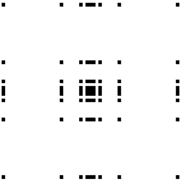
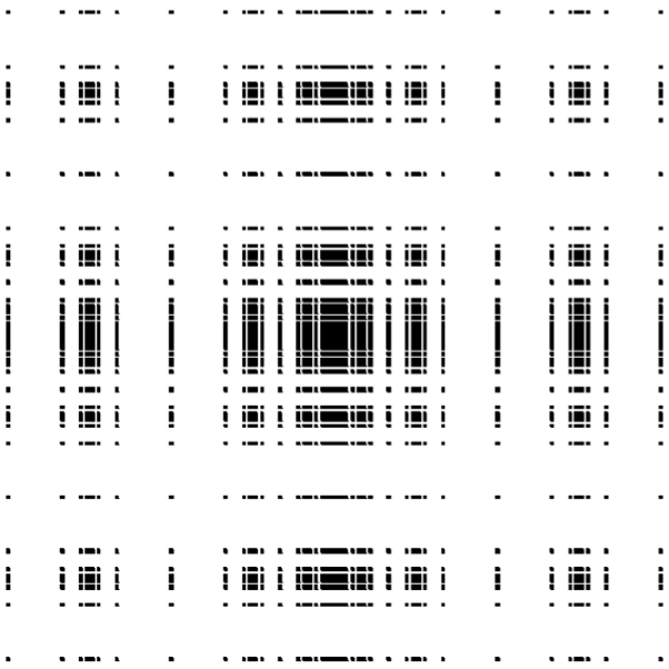
Figure 1. Each cube $Q\in\mathcal{K}^{2}(n_{1},k_{1})$ will be replaced by the affine image of $\mathcal{K}^{2}(n_{2},k_{2})$. We also illustrate one of the many rectangle-skeletons in $\Gamma(n_{1},k_{1})$.

We define

(2.11) $$\Gamma=\operatorname{Sk}\bigl{(}[0,1)^{d}\bigr{)}\ \cup\ \bigcup_{l=1}^{\infty}\ \ \bigcup_{Q\in\mathcal{K}_{l-1}}\ \Gamma_{Q}(n_{l},k_{l})\ \cup\ \bigcap_{l=1}^{\infty}\ K_{l}.$$

Note that $\Gamma$ is connected. The proof of Theorem 1.1 now reduces to the following two propositions, which show that $\mathcal{H}^{1}(\Gamma)<\infty$ and $\nu(\Gamma)>0$ for a certain explicit choice of parameters.

Proposition 2.5 (The length of $\Gamma$).

Let $\delta>0$ and $n_{1}\in\mathbb{Z}$ be parameters so that

(2.12) $$18d[\delta+\delta\log(\delta^{-1})]\leq\log(3)$$

and $k_{1}:=3\delta n_{1}\geq 1$ is an integer. If $\Gamma$ is the curve defined above with parameters $n_{l}=ln_{1}$ and $k_{l}=lk_{1}$, then

(2.13) $$\mathcal{H}^{1}(\Gamma) \leq 3d2^{d}e^{3dn_{1}[\delta+\delta\log(\delta^{-1})]}$$

Proof.

By (2.7) we have

$$\mathcal{H}^{1}\biggl{(}\bigcap_{l=1}^{\infty}K_{l}\biggr{)}\leq\prod_{l=1}^{\infty}\bigl{(}3^{-n_{l}}e^{dk_{l}(1+\log(\delta^{-1})}\bigr{)}=0.$$

Hence by (2.9) and (2.10),

$$\mathcal{H}^{1}(\Gamma) \leq d2^{d-1}+\sum_{l=1}^{\infty}\sum_{Q\in\mathcal{K}_{l-1}}d2^{d}3^{-(n_{1}+\cdots+n_{l-1})}\exp\bigl{\{}dk_{l}[1+\log(\delta^{-1})]\}$$

$$\leq d2^{d}\bigg{[}1+\sum_{l=1}^{\infty}3^{-(n_{1}+\cdots+n_{l-1})}\exp\bigl{\{}(k_{1}+\cdots+k_{l})d[1+\log(\delta^{-1})]\bigr{\}}\biggr{]}.$$

Inserting the values of our parameters and performing a few elementary manipulations, we find

$$\mathcal{H}^{1}(\Gamma_{\!0}) \leq d2^{d-1}e^{3dn_{1}[\delta+\delta\log(\delta^{-1})]}\biggl{[}2+\sum_{l=2}^{\infty}\exp\bigl{\{}-\tfrac{1}{4}l(l-1)\log(3)n_{1}\bigr{\}}\biggr{]}$$

which yields (2.13) with a few more manipulations. ∎

Proposition 2.6 (The measure of $\Gamma$).

Let $\delta$ and $\{n_{l},k_{l}\}_{l=1}^{\infty}$ be as in Proposition 2.5. Then

(2.14) $$\nu(\Gamma)\geq\exp\biggl{\{}-\frac{de^{-2\delta^{2}n_{1}}}{(1-e^{-2\delta^{2}n_{1}})^{2}}\biggr{\}}.$$

Proof.

By the dominated convergence theorem,

$$\nu(\Gamma)\geq\lim_{l\to\infty}\nu\bigl{(}\overline{\cup\,\{Q:Q\in\mathcal{K}_{l}\}}\bigr{)}\geq\lim_{l\to\infty}\nu\bigl{(}\cup\,\{Q:Q\in\mathcal{K}_{l}\}\bigr{)}.$$

(In fact, since doubling measures cannot charge straight lines, equality actually holds above, but we will not need this.) Since the cubes in $\mathcal{K}_{l}$ have disjoint interiors, (2.5) and induction give us

$$\nu\bigl{(}\bigcup\,\{Q:Q\in\mathcal{K}_{l}\}\bigr{)}\geq\bigl{[}1-e^{-2\delta^{2}n_{l}}\bigr{]}^{d}\sum_{Q\in\mathcal{K}_{l-1}}\nu(Q)\geq\prod_{j=1}^{l}\bigl{[}1-e^{-2\delta^{2}n_{j}}\bigr{]}^{d}.$$

Inserting the values of our parameters and performing a few elementary manipulations, we conclude that

$$\nu(\Gamma) \geq\exp\biggl{\{}d\sum_{j=1}^{\infty}\log(1-Z^{j})\biggr{\}}\geq\exp\biggl{\{}-d\sum_{j,k=1}^{\infty}Z^{jk}\biggr{\}}\geq\exp\bigl{\{}-\tfrac{dZ}{(1-Z)^{2}}\bigr{\}}$$

where $Z:=\exp\{-2\delta^{2}n_{1}\}$. That proves (2.14). ∎

In closing, we note that the curve $\Gamma$ can be made to capture an arbitrarily large proportion of the $\nu$-mass of the unit cube; one merely chooses the parameter $n_{1}$ large (with $\delta$ fixed).

References

- [1] G. David and S. Semmes, Analysis of and on uniformly rectifiable sets. Mathematical Surveys and Monographs, 38. American Mathematical Society, Providence, RI, 1993. MR1251061
- [2] K. J. Falconer, The geometry of fractal sets. Cambridge Tracts in Mathematics, 85. Cambridge University Press, Cambridge, 1986. MR0867284
- [3] J.-P. Kahane, Trois notes sur les ensembles parfaits linéaires. Enseignement Math. 15 (1969), 185–192. MR0245734
- [4] E. M. Stein, Harmonic analysis: real-variable methods, orthogonality, and oscillatory integrals. Princeton Mathematical Series, 43. Princeton University Press, Princeton, NJ, 1993. MR1232192
- [5] D. W. Stroock, Probability theory, an analytic view. Cambridge University Press, Cambridge, 1993. MR1267569
- [6] J.-M. Wu, Hausdorff dimension and doubling measures on metric spaces. Proc. Amer. Math. Soc. 126 (1998), 1453–1459. MR1443418