The rolling sphere and the quantum spin

Abstract

We consider the problem of a sphere rolling of a curved surface and solve it by mapping it to the precession of a spin $1/2$ in a magnetic field of variable magnitude and direction. The mapping can be of pedagogical use in discussing both rolling and spin precession, and in particular in understanding the emergence of geometrical phases in classical problems.

I Introduction

In this paper we consider a question similar to that posed in the title of Ref. mont : How much does a sphere rotate when rolling on a curved surface? In Ref. mont , the old problem of the rotation of a torque free, non-spherical body is reanalyzed. The angle of rotation is identified to have two components, one dynamical and one geometrical (the so called Berry phase), independent of the time elapsed during the rotation. Here we consider a related but different problem: a sphere is made to roll without slipping on a given curve $\Gamma$ on a surface. The question is, if the sphere completes a circuit, what is the rotation matrix connecting the initial and final configuration of the sphere? The problem we are considering is therefore a kinematic rather than a dynamic one: the trajectory of the contact point of the sphere and the surface is dictated externally and the rolling constraint is imposed. We make contact with recent approaches that consider the same problem levy1 ; johnson1 (but on a plane), in particular, we address a nice question posed by Brockett and Dai brockett : a sphere lies on a table and is made to rotate by a flat plane on top of it, parallel to the table. The question is: if every point of the plane describes a circle, what is the trajectory and motion of the sphere?

We treat the problem by exploiting its isomorphism to the precession of a spin 1/2 in a time-dependent magnetic field. In the mapping, the arc length of the curve plays the role of time. For rolling on a plane the magnitude of the magnetic field is $1/R$ with $R$ the radius of the sphere, and the direction of the magnetic field is that of the instantaneous angular velocity of the rolling sphere. For a curved surface the normal curvature and the torsion of the curve affect the value of the effective magnetic field. Closely related to the present paper is the use of of the isomorphism between classical dynamics and that of a spin $1/2$ by Berry and Robbins in Ref. berryrobbins , especially their classical view of the Landau-Zener landauzener problem. From a pedagogical perspective, the novel contribution of this paper is to use the isomorphism to discuss rolling spheres on an arbitrary surface.

The precession of a spin $1/2$ is widely treated in the literature and one can borrow those results to acquire an intuition for the rolling sphere. Conversely, since a rolling sphere is a tangible physical problem, the present treatment can be useful pedagogically in presenting spin precession, Berry’s phases and it’s classical counterpart, Hannay’s angle hannay .

II Rolling on a plane and quantum precession

Consider a sphere of radius $R$ rolling on a curve $\Gamma$ on a plane. We define a local triad of unit vectors at the contact point (the so called Darboux frame darboux ): the tangent t to $\Gamma$, the normal n to the surface, and $\textbf{u}=\textbf{n}\times\textbf{t}$, the tangent normal. For rolling on a plane n is a constant vector, and the velocity of the center of the sphere is along the tangent to the curve. This situation will change for rolling on a curved surface, but, as we will see, the general idea of the mapping to a precessing spin is the same.

The translational velocity of the sphere is $\textbf{V}=\textbf{t}V(t)$ and the rolling constraint means that the instantaneous velocity at the contact point is zero landau :

$$\overrightarrow{\omega}\times(\textbf{n}R) = \textbf{V}=\textbf{t}V(t)$$ (1)

with $\overrightarrow{\omega}$ the angular velocity and $R$ the radius of the sphere. This equation is nonintegrable and constitutes a paradigmatic nonholonomic constraint bloch2003 .

Taking the cross product with n on both sides of the above equation we have

$$\overrightarrow{\omega}={V(t)\over R}\textbf{n}\times\textbf{t}\equiv{V(t)\over R}\textbf{u}.$$ (2)

Notice that in the above equation we have used the “no spin” condition $\overrightarrow{\omega}\cdot\textbf{n}=0$, that is, we are consider rolling without an instantaneous rotation along the normal.

The instantaneous velocity $\dot{\textbf{X}}$ of a point of coordinate X (with respect to the center of the sphere) on the surface of the sphere is

$$\dot{\textbf{X}}=\overrightarrow{\omega}\times\textbf{X}={V(t)\over R}\textbf{u}\times\textbf{X}.$$ (3)

Now we rewrite $V(t)=ds/dt$ where $s$ is the arc length of the curve $\Gamma(t)$, and (3) becomes

$${d{\textbf{X}}\over ds}={\textbf{u}\over R}\times\textbf{X}.$$ (4)

If we regard $\textbf{X}=(x,y,z)$ as a magnetic moment, the above equation describes its precession in the presence of a magnetic field $\textbf{B}=-{1\over R}(u_{x},u_{y},u_{z})=-\overrightarrow{\omega}$ of constant magnitude $1/R$. The direction of B is $-\textbf{u}$, and varies varies with $s$, the arc length, which plays the role of time. If the rolling is on a horizontal plane, then $B_{z}$=0, but we keep this notation to make contact with the rolling on an arbitrary surface.

There is an isomorphism between the rolling sphere written in this way with a spin $1/2$ precessing in this magnetic field. This isomorphism can be seen clearly if, (using $\textbf{B}=-\overrightarrow{\omega}$) we rewrite Equation (4) in the form

$${d\over ds}\left(\begin{array}[]{c}x\\ y\\ z\end{array}\right)=\left(\begin{array}[]{ccc}0&B_{z}&-B_{y}\\ -B_{z}&0&B_{x}\\ B_{y}&-B_{x}&0\end{array}\right)\left(\begin{array}[]{c}x\\ y\\ z\end{array}\right),$$ (5)

which is the same as the following equation of motion for two complex numbers $a$ and $b$ (we write $s$ instead of $t$ for time in order to keep the analogy)

$$i{d\over ds}\left(\begin{array}[]{c}a\\ b\end{array}\right)=-{1\over 2}\left(\begin{array}[]{cc}B_{z}&B_{x}-iB_{y}\\ B_{x}+iB_{y}&-B_{z}\\ \end{array}\right)\left(\begin{array}[]{c}a\\ b\end{array}\right),$$ (6)

with the identification

$$x \equiv ab^{*}+ba^{*}$$

$$y \equiv i\left(ab^{*}-ba^{*}\right)$$

$$z \equiv aa^{*}-bb^{*}.$$ (7)

The real numbers $(x,y,z)$ represent the coordinates of a point on the surface of the sphere referred to a coordinate system fixed in space (that is, not rotating), and whose origin is in the center of the sphere. The above mapping is certainly possible because of the $SU(2)-SO(3)$ isomorphism arfken .

Equation (6) is Schrödinger’s equation for the spinor $\chi=(a,b)$ in the presence of a magnetic field B:

$$i{d\over ds}\chi=-\textbf{B}\cdot\textbf{S}\chi\equiv H\chi,$$ (8)

where $\hbar=1$ and $H$ the Hamiltonian. Also, the vector $\textbf{S}={1\over 2}(\sigma_{x},\sigma_{y},\sigma_{z})$ is the spin operator, and $\sigma_{i}$ are Pauli’s matrices. Notice that in this mapping, the magnetic fields and the frequencies have units of inverse length,

Equation (7) implies that we can extract the behavior of the rolling sphere as a function of arc length by solving the motion of a spin $1/2$ in a time-varying magnetic field. To our knowledge the equivalence between the motion of rigid body and a two-level system (a spin $1/2$), in the form of the mapping of Eq. (7) was first pointed out by Feynman, Vernon and Hellwarth Feyn1 and later discussed several times ans . Earlier, Bloch bloch1 had derived the precession equation for the density matrix of spin 1/2 and therefore the points $(x,y,z)$ that result from the mapping from spinors are called the Bloch sphere.

The pedagogical novelty of the present paper (an alternative title of which could well have been “The rolling of the Bloch sphere”) is to discuss the rolling using the arc length as time and identifying the isomorphism between the rolling sphere and the quantum spin in exactly solvable cases.

III Warmup: constant magnetic field

Consider the simplest case of constant magnetic field. We choose $\textbf{B}=B_{0}\hat{\textbf{k}}$, constant in the $+z$ direction. This corresponds to the sphere rolling on a vertical plane. Eq (6) becomes:

$$i{d\over ds}\left(\begin{array}[]{c}a\\ b\end{array}\right)=-{1\over 2}\left(\begin{array}[]{cc}B_{0}&0\\ 0&-B_{0}\\ \end{array}\right)\left(\begin{array}[]{c}a\\ b\end{array}\right),$$ (9)

with solutions:

$$\left(\begin{array}[]{c}a(s)\\ b(s)\end{array}\right) = \left(\begin{array}[]{c}e^{isB_{0}/2}a(0)\\ e^{-isB_{0}/2}b(0)\end{array}\right).$$ (14)

Replacing (14) in (7) we obtain:

$$x(s) = x(0)\cos\left({B_{0}s\over 2}\right)+y(0)\sin\left({B_{0}s\over 2}\right)$$

$$y(s) = y(0)\cos\left({B_{0}s\over 2}\right)-x(0)\sin\left({B_{0}s\over 2}\right)$$

$$z(s) = z(0),$$ (15)

which means that the sphere is rotating clockwise around a constant axis in the $z$ direction. This corresponds to $\overrightarrow{\omega}$ in the $-z$ direction. In other words, a constant magnetic field in the $z$ direction corresponds to the sphere moving in a straight line in the $xy$ plane, rolling on a vertical wall. The same situation applies if a constant field is directed in any other orientation.

IV The lollipop and the planar field

Consider a magnetic field varying on the $xy$ plane as $\textbf{B}=B(\cos\alpha s,\sin\alpha s,0)$. This corresponds to u rotating with the same frequency in the same plane, and the rolling problem becomes that of a sphere of radius $R=1/B$ rolling counterclockwise on a circle of radius $r=1/\alpha$ (see Figure 1).

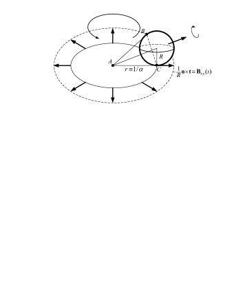
Figure 1: The lollipop, or a sphere rolling counterclockwise on a circle of radius $r$ corresponds to a spin $1/2$ precessing on a magnetic field that rotates in the $xy$ plane.

In turn, this corresponds to a time (or arc length) dependent Hamiltonian $H=-\textbf{B}\cdot\textbf{S}$, which can be solved by noting that

$$\textbf{B}\cdot\textbf{S} = \left(\begin{array}[]{cc}0&Be^{-i\alpha s}\\ Be^{i\alpha s}&0\end{array}\right)=U^{*}\left(\begin{array}[]{cc}0&B\\ B&0\end{array}\right)U,$$ (20)

with

$$U = \left(\begin{array}[]{cc}e^{i\alpha s/2}&0\\ 0&e^{-i\alpha s/2}\end{array}\right).$$ (23)

Substituting the above relations in (6) we obtain a time independent equation for the coefficients $\tilde{\chi}(s)=(\tilde{a},\tilde{b})=(e^{i\alpha s/2}a,e^{-i\alpha s/2}b)$

$$i{d\over ds}\left(\begin{array}[]{c}\tilde{a}\\ \tilde{b}\end{array}\right)=-{1\over 2}\left(\begin{array}[]{cc}\alpha&B\\ B&-\alpha\\ \end{array}\right)\left(\begin{array}[]{c}\tilde{a}\\ \tilde{b}\end{array}\right)\equiv\tilde{H}\left(\begin{array}[]{c}\tilde{a}\\ \tilde{b}\end{array}\right).$$ (24)

Transformations (20) and (23) correspond to transforming to a frame that rotates with angular velocity $\alpha$ slichter . When transforming to the rotating frame, the angular velocity acquires a component $\alpha=1/r$ in the $z$ direction and the frequency of rotation in the rotating frame is

$$\Omega=\sqrt{B^{2}+\alpha^{2}}={1\over rR}\sqrt{r^{2}+R^{2}}$$ (25)

This can be seen in the spinor language by noting that, since $\tilde{H}$ in Eq. (24) is time-independent , the solutions are

$$\tilde{\chi}(s) = e^{{i\over 2}s\left(\begin{array}[]{cc}\alpha&B\\ B&-\alpha\\ \end{array}\right)}\tilde{\chi}(0)$$ (28)

$$= \left[\cos\left({\Omega s/2}\right)+i\vec{\sigma}\cdot\textbf{m}\sin\left({\Omega s/2}\right)\right]\tilde{\chi}(0),$$ (29)

with $\pm\Omega=\sqrt{B^{2}+\alpha^{2}}$ the eigenvalues of $\tilde{H}$ and m a unit vector in the direction $\alpha/B=R/r$. Equation (29) describes a rotation at a rate $\Omega$ with respect to an axis in the direction of the “stick” of the lollipop (the direction joining $A$ to the center of the sphere (see Fig. (1)). Notice that solving for the evolution by exponentiating $\tilde{H}$ is possible because $\tilde{H}$ does not depend on $s$. If there is an $s$-dependence and the matrices $\tilde{H}$ at different $s$ do not commute the solution is a “time ordered” exponential that in general is not exactly solvable.

After the lollipop completes a circle, the angle $\delta$ of rotation is

$$\delta={2\pi\over\alpha}\Omega=2\pi\sqrt{1+\left({r\over R}\right)^{2}}.$$ (30)

Notice that, when $R\ll r$ the angle of rotation is $\delta=2\pi r/R$, corresponding to rolling in a line of length equal to the perimeter of the circle.

In anticipation of the next section we mention than in this case, since the rolling is on the plane, there is no geometric phase. When the rolling is on a curved surface the situation changes. Notice that we are using the term “geometric phase” in its relation with the spin problem in the adiabatic approximation. This phase is different from the nonholonomy when the sphere of arbitrary radius describes a loop.

We see that, after traveling on a circle the sphere is rotated by $2\pi\Omega/\alpha$ with respect to an axis tilted with respect to the plane; this is the nonholonomy treated in johnson1 and iwai .

When the sphere rolls on a plane, and on a circle of radius $r$ much larger than its radius $R$, it comes back rotated around an axis that lies on the plane, by an angle given only by the dynamical phase. The extra term that originates in the curvature of the surface is what we call the geometric phase.

The angle of rotation $\delta$ (of both the spin and the lollipop) has a simple geometric interpretation: when the lollipop rolls, the point of contact $C$ moves on the circular rim of the cone $ABC$ (see Figure 1). At the same time, the point $C$ “paints” on the sphere a circle of diameter $BC=2rR/\sqrt{r^{2}+R^{2}}$. (This is easily calculated with simple geometrical considerations from Figure 1.) This means that after a revolution of length $2\pi r$ the angle rotated is $2\pi r/(BC/2)$ from which Eq. (30) follows immediately.

At this point we consider Brockett’s question mentioned in the Introduction. Notice first that, as the sphere rolls on a circle, the velocity at the top of the sphere is twice the velocity V at the center of the sphere. Since each point of the plane on top of the sphere describes a circle of radius $R_{1}$, the velocity $\textbf{V}_{P}$ of the plane also describes a circle. Therefore, since the sphere has a rolling condition with the upper plane, then $\textbf{V}_{P}=2\textbf{V}$, meaning that, as the plane describes a circle of radius $R_{1}$ the sphere describes a circle of radius $R_{1}/2$.

We showed this with a nice classroom demo: on a piece of paper draw a circle of radius 5 inches (twice that of a tennis ball). Orient the label of the tennis ball at 45 degrees with the vertical (the sphere is going to roll on a circle of radius $r=R$, and therefore the axis of rotation is going to be at 45 degrees and the precession frequency will be, from (25), $\sqrt{2}$). Paint a mark on a transparent glass, which in turn will serve as the upper plane. Also mark three points on the circle separated by $\beta=127$ degrees ($\pi/\sqrt{2}$). Looking through the glass, guide the mark on the glass over the circle on the paper, and notice that, each time the glass rotates by $\beta$, the tennis ball rotates by $\pi$ with respect to a moving axis at 45 degrees.

Notice also that for $s=2\pi/\alpha$ the spinor $\chi$ changes sign due to the $1/2$ factor in the transformation. Nevertheless, since the mapping of (7) is quadratic in $a$ and $b$, changing their signs corresponds to the same values $(x,y,z)$ for the orientations. More specifically, the quantities $a$ and $b$ determine univocally $x,y$ and $z$, but the reverse is not valid: the quantum evolution determines univocally the classical evolution but there is some ambiguity in going from the classical to the quantum case. For example if we perform the “gauge transformation” $(a,b)\rightarrow e^{i\phi(s)}(a,b)$ the mapping to the X coordinate remains unchanged.

We will come back to this point in the next sections when we discuss the geometric phase for rolling.

V rolling on a curved surface

In this section we extend the treatment of rolling on a plane to rolling on a curved surface (See Figure 2). If we call $\textbf{X}_{P}$ the coordinate of the contact point, the coordinate $\textbf{X}_{c}$ of the center of the sphere is:

$$\textbf{X}_{c}=\textbf{X}_{P}+R\textbf{n},$$ (31)

and its velocity is given by

$$\dot{\textbf{X}}_{c} = \dot{\textbf{X}}_{P}+R\dot{\textbf{n}},$$ (32)

$$= \left(\textbf{t}+R{d\textbf{n}\over ds}\right){ds\over dt}.$$

The rolling condition is that the velocity of a point of the sphere in contact with the surface is zero (See Eq.(1)):

$$\overrightarrow{\omega}\times(\textbf{n}R)=\dot{\textbf{X}}_{c}.$$ (33)

Again, taking the cross product with n on both sides of the equation above we obtain

$$\overrightarrow{\omega}={1\over R}\textbf{n}\times\dot{\textbf{X}}_{c}.$$ (34)

We now replace (32) in (34), and use the fact that, for a curved surface, the variation of the normal is given by

$${d\textbf{n}\over ds}=-\kappa_{n}\textbf{t}-\tau_{r}\textbf{u},$$ (35)

with $\kappa_{n}$ the normal curvature and $\tau_{r}$ the torsion of the curve, both evaluated at the contact point. We obtain

$$\overrightarrow{\omega}=\left[{1\over R}\left(1-\kappa_{n}R\right)\textbf{u}+{\tau_{r}}\textbf{t}\right]{ds\over dt}.$$ (36)

The discussion for the planar case extends to the curved surface, and the rolling of the sphere is equivalent to a spin $1/2$ precessing on a magnetic field $\textbf{B}(s)$ given by

$$\textbf{B}(s)=-\left[{1\over R}\left(1-\kappa_{n}R\right)\textbf{u}+{\tau_{r}}\textbf{t}\right],$$ (37)

with the arc length $s$ playing the role of time. In the following section, as an example of this formulation we consider rolling on a spherical surface.

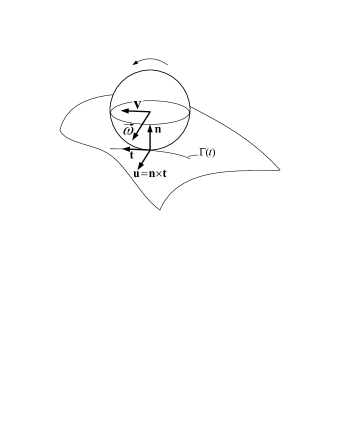
Figure 2: Sphere rolling along a curve $\Gamma$ of zero torsion (meaning that the velocity of the center of the sphere is parallel to the tangent of the curve at the contact point).

VI sphere rolling on a spherical surface

In this section we consider a sphere of radius $R$ rolling on a second sphere of radius $r$. The rolling line will be a parallel of latitude $\pi/2-\theta$ (see Figure 3). This means that the normal curvature is constant $1/r$, and also that the torsion is zero. The magnetic field for the corresponding spin problem is therefore:

$$\textbf{B}(s)=-\left[{1\over R}\left(1\pm{R\over r}\right)\textbf{u}\right]=-{1\over\widetilde{R}_{\pm}}\textbf{u},$$ (38)

with $\widetilde{R}_{\pm}=rR/(r\pm R)$ a reduced radius and the plus and minus signs refer to the rolling outside and inside of the sphere of radius $r$ respectively.

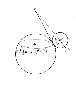
Figure 3: Sphere rolling on a sphere.

For a sphere rolling on a parallel, the instantaneous angular velocity (and the magnetic field) describes a cone forming an angle $\theta$ with the vertical. The total arc length of the parallel is $r\sin\theta$ meaning that the vector u rotates with angular frequency $\alpha$ given by $\alpha=1/(r\sin\theta)$. The corresponding magnetic field is therefore

$$\textbf{B}(s)=(B_{x},B_{y},B_{z})={1\over\widetilde{R}_{\pm}}(\cos\theta\cos\alpha s,\cos\theta\sin\alpha s,-\sin\theta)$$ (39)

with the term $\textbf{B}\cdot\textbf{S}$ in the corresponding Hamiltonian given in this case by

$$\textbf{B}\cdot\textbf{S} = {1\over 2}{1\over\widetilde{R}_{\pm}}\left(\begin{array}[]{cc}-\sin\theta&\cos\theta e^{-i\alpha s}\\ \cos\theta e^{i\alpha s}&\sin\theta\end{array}\right).$$ (42)

This again is an exactly solvable Hamiltonian that was first studied by Rabi

Using the same transformation matrix of Eq. (23) the above Hamiltonian can be rendered time independent. We write it in the following form

$$\tilde{H} = -{1\over 2}\left(\begin{array}[]{cc}-B_{0}\sin\theta+\alpha&B_{0}{\cos\theta}\\ B_{0}{\cos\theta}&B_{0}{\sin\theta}-\alpha\end{array}\right),$$ (45)

with $B_{0}=1/\widetilde{R}_{\pm}$.

The eigenvalues of $\tilde{H}$ are

$$\Omega_{\pm} = {1\over\widetilde{R}_{\pm}}\sqrt{1-{2\widetilde{R}_{\pm}\over r}+\left({\widetilde{R}_{\pm}\over r\sin\theta}\right)^{2}},$$ (46)

with the spinor precessing, in the rotating frame, around an axis that forms an angle $\beta$ (see Figure 3) with the $xy$ plane, with

$$\tan\beta=\tan\theta-{R\over r+R}{1\over\sin\theta\cos\theta}$$ (47)

The second term in (47) reflects the fact that the small sphere rotates instantaneously on the tangent plane that contains $BC$ (see Figure 3). Equation (47) can be easily derived by simple geometric considerations from Figure (3).

After a complete revolution the angle or rotation $\delta$ is

$$\delta_{\pm}=2\pi r\sin\theta\Omega_{\pm}.$$ (48)

After a little algebra we obtain

$$\delta_{+} = 2\pi\cos\theta\sqrt{1+\left({r\tan\theta\over R}\right)^{2}},$$

$$\delta_{-} = 2\pi\sqrt{1+\sin^{2}\theta{(r-3R)(r-R)\over R^{2}}}.$$ (49)

Notice that, if we compare with the rotation in a plane from Eq. (25), the “outer” rotation corresponds to rolling on a circle of radius equal to that of the unfolded cone tangent to the parallel (See Fig. 3). The angle of rotation along that circle is not $2\pi$ but $2\pi\cos\theta$. This geometric factor is the same that appears in Foucault’s pendulum and in Berry’s phase for a spin precessing on a cone (we will come back to this point below). Also, notice that when $r=R$ the angle of rotation is always $2\pi$ independent of latitude.

The “inner” roll has the interesting feature that, when $r=3R$ the angle of rotation is $2\pi$ regardless of latitude. This amusing feature can be verified easily at the equator: roll a penny inside of a circle of radius three times the radius of the penny and verify that the penny completes a full rotation in the rotating frame (and of course two full rotations in the lab frame).

We finish this section with a discussion of the differences and similarities between the Berry phase for a precessing spin $1/2$ in the adiabatic approximation and the rolling of two spheres.

The Hamiltonian for a spin in a magnetic field that precesses along the $z$ axis at frequency $\alpha$ is given by (45), where in principle $\alpha$ and $B_{0}$ are independent parameters. If $\alpha\ll B_{0}$ (the adiabatic approximation) the eigenvalues (eigenfrequencies) of $\widetilde{H}$ are

$$\Omega\simeq\sqrt{B_{0}^{2}-2\alpha B_{0}\sin\theta}\simeq B_{0}-\alpha\sin\theta.$$ (50)

After a period of time $2\pi/\alpha$ the change $\Delta\phi$ in the phase of the spin is

$$\Delta\phi=2\pi{B_{0}\over\alpha}-2\pi\sin\theta.$$ (51)

The first therm is the dynamical phase and the second is a purely geometrical one, independent of the parameters $B_{0}$ and $\alpha$, and give by (half) the solid angle described by the field.

For the rolling sphere we can also study an “adiabatic approximation” since $\alpha\ll B_{0}$ corresponds to $r\gg R$. In other words, in general the adiabatic approximation will correspond to the radius of the rolling sphere much smaller than the radius of curvature of the surface. On the other hand, in contrast with the spin case, the frequency of rotation $\alpha=1/r\sin\theta$ “knows” about the latitude and the curvature. So we expect some differences and some similarities. Replacing the values of $B_{0}=1/\widetilde{R}_{\pm}\equiv 1/R\pm 1/r$ in (51) we obtain the angle of rotation of the sphere in each case (in the adiabatic approximation)

$$\Delta\phi_{\pm} = 2\pi r\sin\theta\left({1\over R}\pm{1\over r}\right)-2\pi\sin\theta.$$ (54)

$$= \left\{\begin{array}[]{cc}2\pi{r\sin\theta\over R}&{\rm{(Outer\;\;rolling)}},\\ 2\pi{r\sin\theta\over R}-4\pi\sin\theta&{\rm{(Inner\;\;rolling)}}\end{array}\right.$$

The above interplay of curvatures for inner and outer rolling is a special case of more general treatments of kinematics of rolling and is discussed in Ref. montana .

From Eq. (54), we see that in the outer rolling case there is no Berry phase, something we could have expected because of the analogy with the rolling on a flat plane. The angle of rotation is in this case given simply by the rotation on a straight line of length equal to the perimeter of the parallel. However, for the inner rolling we indeed have a geometric phase twice as big as that of the spin $1/2$. Our treatment is a nice example of the appearance of a geometric phase in a classical system, originally discussed by Hannay hannay .

In the next section we discuss the general connection between rolling and the Berry phase for spins in the adiabatic approximation.

VII The adiabatic approximation and rolling on a curved surface

In this section we compare the equivalence between the adiabatic approximation for a spin precessing in a magnetic field that changes direction at a slow rate and rolling on a surface. In the spin case, the dimensionless parameter controlling the approximation is the ratio of the instantaneous frequency (proportional to the instantaneous magnitude of the field) with the rate at which it’s direction is changing.

In the rolling case the instantaneous frequency corresponds to the magnitude of $\textbf{B}(s)$ and the rate of change in its direction is related to the normal curvature and to the curve’s torsion.

In the adiabatic approximation for spins sakurai , one works in an “instantaneous” basis, treating first $s$ (time) as a parameter and solving the eigenvalue equation as though the problem were static:

$$H(s)\chi(s)=\Omega(s)\chi(s).$$ (55)

Then the general solution is written as linear combinations of the instantaneous eigenstates. As a result, in the adiabatic approximation, the spinor at time $s$ is given by

$$\chi(s)=e^{i\gamma(s)}e^{i\int_{0}^{s}ds^{\prime}\Omega(s^{\prime})}\chi(0).$$ (56)

The argument of the second exponential above represents the dynamic phase, which involves the integral of the following angular frequency:

$$\Omega(s) = |\textbf{B}(s)|={1\over R}\sqrt{\left[1-\kappa_{n}(s)R\right]^{2}+[\tau(s)R]^{2}}$$ (57)

$$\simeq {1\over R}-\kappa_{n}(s)$$

This can be seen, for example from Equation (42): the eigenvalues of $\textbf{B}\cdot\textbf{S}$ with $s$ treated as a parameter are $\pm|\textbf{B}(s)|$.

The (instantaneous) direction of the field is in the direction $\textbf{u}_{B}$ given by

$$\textbf{u}_{B}={\textbf{B}(s)\over|\textbf{B}(s)|}=-{\left(1-\kappa_{n}R\right)\textbf{u}+{\tau_{r}}\textbf{t}\over\sqrt{\left(1-\kappa_{n}R\right)^{2}+\tau_{r}^{2}}}$$ (58)

In general, the eigenvalues of a Pauli matrix in an arbitrary direction $\textbf{u}_{B}\cdot\vec{\sigma}$ given by the unit vector $\textbf{u}_{B}=(u_{x},u_{y},u_{z})$ are $\pm 1$. This is verified by noting that (defining $u_{x}+iu_{y}=\rho e^{i\phi}$)

$$\left(\textbf{u}_{B}\cdot\vec{\sigma}\right)\chi_{\pm}(\textbf{u}_{B})=\left(\begin{array}[]{cc}u_{z}&\rho e^{-i\phi}\\ \rho e^{i\phi}&-u_{z}\end{array}\right)\chi_{\pm}(\textbf{u}_{B})=\pm\chi_{\pm}(\textbf{u}_{B}),$$ (59)

with $\chi_{\pm}(\textbf{u}_{B})=(1,\pm(1-u_{z})e^{\pm i\phi}/\rho)$. Notice that the dependence of $\chi$ on $s$ is through the orientation of u.

The first term, the geometric phase $\gamma$, is the Berry phase, and is given by

$$\gamma(s)=\int_{0}^{s}ds^{\prime}\chi(\textbf{u}_{B}(s^{\prime}))^{\dagger}{d\over ds^{\prime}}\chi(\textbf{u}_{B}(s^{\prime})).$$ (60)

If the rolling describes a complete circuit, $\gamma$ measures the solid angle described by $\textbf{u}_{B}$. This can be seen explicitly as follows. If we express $\textbf{u}_{B}$ in polar coordinates $\textbf{u}_{B}=(\sin\theta\cos\phi,\sin\theta\cos\phi,\cos\theta)$ then the spinor in that direction is:

$$\chi(\textbf{u}_{B}(s))=\left(\begin{array}[]{c}\cos{\theta(s)\over 2}e^{-i\phi(s)/2}\\ \sin{\theta(s)\over 2}e^{i\phi(s)/2}\end{array}\right).$$ (61)

This means that $\chi^{\dagger}{d\over ds^{\prime}}\chi=-{1\over 2}\cos{\theta}{d\phi\over ds^{\prime}}$, and the integral over a closed circuit $\Gamma$ can be written as

$$\gamma_{\Gamma}=-{1\over 2}\oint_{\Gamma}\textbf{A}\cdot d\textbf{l},$$ (62)

with $\textbf{A}={\cos{\theta}\over\sin{\theta}}\textbf{u}_{\phi}$. Since $\nabla\times\textbf{A}=-\textbf{u}_{r}$, using Stokes theorem, the line integral of A is the flux of a monopole in the origin, giving the solid angle holstein .

Notice that this solid is traced not by the normal to the surface but by $\textbf{u}_{B}$. This means that the solid angle measures a combination of the normal curvature and the torsion of the curve. In contrast, the solid angle traced by the normal measures the geodesic curvature levy2 . In summary, we have shown that, when a sphere of radius $R$ rolls on a surface of local radius of curvature and inverse torsion much larger than $R$, the angle of rotation $\delta$ in a closed curve of length $L$ is given by

$$\delta={L\over R}-\int_{0}^{L}ds\kappa_{n}(s)-S,$$ (63)

with $S$ the solid angle traced by $\textbf{u}_{B}$. Note that, if we specify this result to the sphere rolling on the parallel of a sphere of radius $r$, we have $L=2\pi r\sin\theta$, $\kappa_{n}=\pm 1/r$ (for inner and outer rolling respectively) and $S=2\pi\sin\theta$. Replacing these in Eq. (63) we obtain the result of Eq. (54) as expected.

VIII acknowledgments

We thank Michael V. Berry for useful comments on the manuscript and for pointing us to Ref berryrobbins . We thank Roger Brockett and Paul R. Berman for interesting remarks. A.G.R thanks the Research Corporation, and A.M.B. thanks the National Science Foundation for support.

References

- (1) R. Montgomery, “How much does a rigid body rotate? A Berry’s phase from the 18th century”. Am. J. Phys, 59, pp. 394-398 (1991).
- (2) M. Levy, “Geometric Phases in the Motion of Rigid Bodies”, Arc. Rational. Mech. Anal. 122, pp. 213-229 (1993).
- (3) B. D. Johnson, “The nonholonomy of the rolling sphere”, The American Mathematical Monthly, 114, pp. 500-508 (2007).
- (4) R. Brockett and L. Dai, “Non-holonomic kinematics and the role of elliptic functions in constructive controllability”, in Z. Li and J. Canny (eds), Nonholonomic Motion Planning, Kluwer, 1993.
- (5) M. V. Berry and J. M. Robins, “Classical Geometrical forces of reaction: an exactly solvable model”. Proc. Roy. Soc. Lond. A 442 pp. 641-658 (1993).
- (6) J. H. Hannay, “Angle Variable Holonomy in Adiabatic Excursions of an Integrable Hamiltonian”, J. Phys. A18 pp. 221-230 (1985). Also reprinted in wilgeom .
- (7) C. Zener, ”Non-adiabatic Crossing of Energy Levels”. Proc. Roy. Soc. Lond. A 137 pp.692 702 (1932).
- (8) H. Guggenheimer, “Differential Geometry” (Chapter 10. “Surfaces”. Dover (1977).
- (9) L. D. Landau and E. M. Lifshitz, “Mechanics”, Third Edition, p. 123, Butterworth-Heineman, Amsterdam, (2003).
- (10) A. M. Bloch, ,with J. Baillieul, P. Crouch and J.E. Marsden, “Nonholonomic Mechanics and Control”, Springer Verlag, 2003.
- (11) G. B. Arfken and H. J. Weber, “Mathematical Methods for Physicists”, Academic Press, pp. 232-236 (1995).
- (12) R. P. Feynman, F. L. Vernon and R. W. Hellwarth, “Geometrical Representation of the Shrödinger Equation for Solving Maser Problems”, J. Appl. Phys, 28, pp. 49-52 (1957).
- (13) F. Bloch, “Nuclear Induction”, Phys. Rev. 70, pp. 460-474 ( 1946).
- (14) I. I. Rabi, “Space Quantization in a Gyrating Magnetic Field”, Phys. Rev. 51 pp. 652-654 (1937).
- (15) See for example F. Ansbacher, “A note on the equivalence of the classical motion of rigid bodies with prescribed angular velocities and the quantum mechanical solutions for paramagnetic atoms in external fields”, J. Phys. B: Atom. Molec. Phys. 6, pp. 1616-1619 (1973); H. Urbantke, “Two-level systems: States, phases and holonomy”, Am. J. Phys. 59, pp. 504-509 (1991), and D. J. Siminovitch, “Rotations in NMR: Part I. Euler Rodrigues Parameters and Quaternions”, Concepts Magn. Reson., 9 pp. 149-171 (1997).
- (16) “Geometric Phases in Physics”, edited by A. Shapere and F. Wilczek (World Scientific, Singapore, 1989).
- (17) T. Iwai and E. Watanabe, “The Berry phase in the plate-ball problem”, Phys. Lett. A, 225 pp. 183-187 (1997).
- (18) See for example C. P. Slichter, “Principles of Magnetic Resonance, Third Edition”, pp. 25-35 (Springer-Verlag, Berlin, 1990)
- (19) For more ellaborate treatments see G. Bor and R. Montgomery, “ and the ”Rolling Distribution”, preprtint arXiv:math/0612469v1, and J.E. Marsden, R. Montgomery, and T.S. Ratiu, “Reduction, Symmetry and Phase in Mechanics”, Memoirs of the American Mathematical Society, Providence, RI, vol 436, (1990).
- (20) J. J. Sakurai, “Modern Quantum Mechanics”, (Addison-Wesley, New York), pp. 464-468
- (21) M. V. Berry, “Quantal Phase Factors Accompanying Adiabatic Changes”. Proceedings of the Royal Society of London, A, 392, pp. 45–56 (1984)
- (22) D. J. Montana, “The Kinematics of Contact and Grasp”, The International Journal of Robotics Research, 7, pp.17-32 (1988).
- (23) For a more detailed discussion see B. R. Holstein, “The adiabatic theorem and Berry’s phase”, Am. J. Phys. 57 pp.1079-1084 (1989).
- (24) For a related discussion see M. Levi. “A ‘bicycle wheel’ proof of the Gauss-Bonnet theorem”. Expositiones Mathematicae, 12, pp.145-164. (1993).