Three-loop HTL Free Energy for QED

Abstract

We calculate the free energy of a hot gas of electrons and photons to three loops using the hard-thermal-loop perturbation theory reorganization of finite-temperature perturbation theory. We calculate the free energy through three loops by expanding in a power series in $m_{D}/T$, $m_{f}/T$, and $e^{2}$, where $m_{D}$ and $m_{f}$ are thermal masses and $e$ is the coupling constant. We demonstrate that the hard-thermal-loop perturbation reorganization improves the convergence of the successive approximations to the QED free energy at large coupling, $e\sim 2$. The reorganization is gauge invariant by construction, and due to cancellation among various contributions, we obtain a completely analytic result for the resummed thermodynamic potential at three loops. Finally, we compare our result with similar calculations that use the $\Phi$-derivable approach.

I Introduction

The thermodynamic functions for hot field theories can be calculated as a power series in the coupling constant $g$ at weak coupling. One is primarily interested in calculating the free energy from which the pressure, energy density, and entropy can be obtained using standard thermodynamic relations. In the early 1990s the free energy was calculated to order $g^{4}$ in Refs. wrong ; AZ-95 for massless scalar $\phi^{4}$ theory, in Ref. qed4 for QED and in Ref. AZ-95 for non-Abelian gauge theories. The corresponding calculations to order $g^{5}$ were carried out in Refs. singh ; ea1 , Refs. parwani ; Andersen and Refs. KZ-96 ; BN-96 , respectively. Recent results have extended the calculation of the QCD free energy by determining the coefficient of the $g^{6}\log(g)$ contribution Kajantie:2002wa . For massless scalar $\phi^{4}$ the perturbative free energy is now known to order $g^{6}$ Gynther:2007bw and $g^{8}\log(g)$ Andersen:2009ct .

Unfortunately, the resulting weak-coupling approximations, truncated order-by-order in the coupling constant, are poorly convergent unless the coupling constant is extremely small. For example, simply comparing the magnitude of low-order contributions to the $N_{f}=3$ QCD free energy one finds that the $g_{s}^{3}$ contribution is smaller than the $g_{s}^{2}$ contribution only for $g_{s}\mathrel{\hbox to0.0pt{\lower 4.0pt\hbox{\hskip 1.0pt$\sim$}\hss}\raise 1.0pt\hbox{$<$}}0.9$ ($\alpha_{s}\mathrel{\hbox to0.0pt{\lower 4.0pt\hbox{\hskip 1.0pt$\sim$}\hss}\raise 1.0pt\hbox{$<$}}0.07$). This is a troubling situation since at phenomenologically accessible temperatures near the critical temperature for the QCD deconfinement phase transition, the strong coupling constant is on the order of $g_{s}\sim 2$. We therefore need methods which can provide reliable approximations to QCD thermodynamics at intermediate coupling.

The poor convergence of finite-temperature perturbative expansions of the free energy is not limited to QCD. The same behavior can be seen in weak-coupling expansions in scalar field theory spt and QED parwani ; Andersen . In Fig. 1 we show the successive perturbative approximations to the QED free energy. As can be seen from this figure, at couplings larger than $e\sim 1$ the QED weak-coupling approximations also exhibit poor convergence. For this reason a concerted effort has been put forth to find a reorganization of finite-temperature perturbation theory which converges at phenomenologically relevant couplings. Here we will focus on the QED free energy.

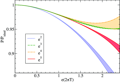
Figure 1: Successive perturbative approximations to the QED pressure (negative of the free energy). Each band corresponds to a truncated weak-coupling expansion accurate to order $e^{2}$, $e^{3}$, $e^{4}$, and $e^{5}$, respectively. Shaded bands correspond to variation of the renormalization scale $\mu$ between $\pi T$ and $4\pi T$.

There are several ways of systematically reorganizing the perturbative expansion to improve its convergence and the various approaches have been reviewed in Refs. birdie ; kraemmer ; review . Here we will focus on the hard-thermal-loop perturbation theory (HTLpt) method htl1 ; AS-01 ; fermions ; htl2 ; aps1 . The HTLpt method is inspired by variational perturbation theory yuk ; steve ; kleinert ; deltaexp . HTLpt is a gauge-invariant extension of screened perturbation theory (SPT) K-P-P-97 ; CK-98 ; spt ; Andersen:2008bz , which is a perturbative reorganization for finite-temperature massless scalar field theory. In the SPT approach, one introduces a single variational parameter which has a simple interpretation as a thermal mass. In SPT a mass term is added to and subtracted from the scalar Lagrangian, with the added piece kept as part of the free Lagrangian and the subtracted piece associated with the interactions. The mass parameter is then required to satisfy a variational equation which is obtained by the principle of minimal sensitivity.

This naturally led to the idea that one could apply a similar technique to gauge theories by adding and subtracting a mass in the Lagrangian. However, in gauge theories, one cannot simply add and subtract a local mass term since this would violate gauge invariance. Instead one adds and subtracts to the Lagrangian a hard-thermal-loop (HTL) improvement term. The free part of the Lagrangian then includes the HTL self-energies and the remaining terms are treated as perturbations. Hard-thermal-loop perturbation theory is a manifestly gauge-invariant approach that can be applied to static as well as dynamic quantities. SPT and HTLpt have been applied to four and two loops spt ; Andersen:2008bz ; AS-01 ; htl1 ; fermions ; htl2 ; aps1 , respectively, and convergence is improved compared to the weak-coupling expansion.

In this paper we calculate the pressure in QED to three-loop order in HTLpt. This will set the stage for the corresponding calculation in full QCD. We determine leading-order (LO), next-to-leading-order (NLO), and next-to-next-to-leading-order (NNLO) expressions for the HTLpt pressure. At NNLO the expression is entirely analytic and gives a well-defined gap equation (variational equation) for the electron and photon screening masses. As we will show, the NLO and NNLO HTLpt resummed QED free energy give approximations which show improved convergence for couplings as large as $e\sim 2.5$ (see Fig. 7). In addition, we compare our results to those obtained using the 2PI $\Phi$-derivable approach phijm ; Borsanyi:2007bf and show that at three loops the agreement between the HTLpt and $\Phi$-derivable approaches is quite good.

The structure of the paper is as follows. We give a brief summary of HTLpt in Sec. II. In Sec. III, we list the expressions for the one-, two-, and three-loop diagrams that contribute to the thermodynamic potential. In Sec. IV, we expand the sum-integrals in the mass parameters, and in Sec. V, the free energy is calculated. We summarize and draw our conclusions in Sec. VI. In Appendix A, we give the Feynman rules for HTLpt in Minkowski space. In Appendixes B and C, we list all sum-integrals and integrals needed in the calculations.

II HTL perturbation theory

The Lagrangian density for massless QED in Minkowski space is

$${\cal L}_{\rm QED} = -{1\over 4}F_{\mu\nu}F^{\mu\nu}+i\bar{\psi}\gamma^{\mu}D_{\mu}\psi$$ (1)

$$\hskip 25.60747pt+{\cal L}_{\rm gf}+{\cal L}_{\rm gh}+\Delta{\cal L}_{\rm QED}\;.$$

Here the field strength is $F^{\mu\nu}=\partial^{\mu}A^{\nu}-\partial^{\nu}A^{\mu}$ and the covariant derivative is $D^{\mu}=\partial^{\mu}+ieA^{\mu}$. The ghost term ${\cal L}_{\rm gh}$ depends on the gauge-fixing term ${\cal L}_{\rm gf}$. In this paper we choose the class of covariant gauges where the gauge-fixing term is

$${\cal L}_{\rm gf} = -{1\over 2\xi}\left(\partial_{\mu}A^{\mu}\right)^{2}\;,$$ (2)

with $\xi$ being the gauge-fixing parameter. In this class of gauges, the ghost term decouples from the other fields.

The perturbative expansion in powers of $e$ generates ultraviolet divergences. The renormalizability of perturbative QED guarantees that all divergences in physical quantities can be removed by renormalization of the coupling constant $\alpha=e^{2}/4\pi$. There is no need for wavefunction renormalization, because physical quantities are independent of the normalization of the field. There is also no need for renormalization of the gauge parameter, because physical quantities are independent of the gauge parameter.

Hard-thermal-loop perturbation theory is a reorganization of the perturbation series for thermal gauge theories. In the case of QED, the Lagrangian density is written as

$${\cal L}=\left({\cal L}_{\rm QED}+{\cal L}_{\rm HTL}\right)\Big{|}_{e\to\sqrt{\delta}e}+\Delta{\cal L}_{\rm HTL}\;.$$ (3)

The HTL improvement term is

$${\cal L}_{\rm HTL}=-{1\over 2}(1-\delta)m_{D}^{2}F_{\mu\alpha}\left\langle{y^{\alpha}y^{\beta}\over(y\cdot\partial)^{2}}\right\rangle_{\!\!y}F^{\mu}_{\;\;\beta}$$

$$+(1-\delta)\,im_{f}^{2}\bar{\psi}\gamma^{\mu}\left\langle{y^{\mu}\over y\cdot D}\right\rangle_{\!\!y}\psi\,,$$ (4)

where $y^{\mu}=(1,\hat{{\bf y}})$ is a light-like four-vector, and $\langle\ldots\rangle_{y}$ represents an average over the directions of $\hat{{\bf y}}$. The term (4) has the form of the effective Lagrangian that would be induced by a rotationally-invariant ensemble of charged sources with infinitely high momentum. The parameter $m_{D}$ can be identified with the Debye screening mass and the parameter $m_{f}$ can be identified as the induced finite-temperature electron mass. HTLpt is defined by treating $\delta$ as a formal expansion parameter.

The HTL perturbation expansion generates ultraviolet divergences. In QED perturbation theory, renormalizability constrains the ultraviolet divergences to have a form that can be cancelled by the counterterm Lagrangian $\Delta{\cal L}_{\rm QED}$. We will demonstrate that renormalized perturbation theory can be implemented by including a counterterm Lagrangian $\Delta{\cal L}_{\rm HTL}$ among the interaction terms in (3). There is no proof that the HTL perturbation expansion is renormalizable, so the general structure of the ultraviolet divergences is not known; however, it was shown in previous papers htl2 ; aps1 that it was possible to renormalize the next-to-leading-order HTLpt prediction for the free energy of QED using only a vacuum counterterm, a Debye mass counterterm, and a fermion mass counterterm. In this paper we will show that renormalization is also possible at NNLO.

The counterterms necessary are

$$\delta\Delta\alpha = N_{f}{\alpha^{2}\over 3\pi\epsilon}\delta^{2}\;,$$ (5)

$$\Delta m_{D}^{2} = N_{f}\left({\alpha\over 3\pi\epsilon}+{\cal O}(\delta^{2}\alpha^{2})\right)(1-\delta)m_{D}^{2}\;,$$ (6)

$$\Delta m_{f}^{2} = \left(-{3\alpha\over 4\pi\epsilon}+{\cal O}(\delta^{2}\alpha^{2})\right)(1-\delta)m_{f}^{2}\;,$$ (7)

$$\Delta{\cal E}_{0} = \left({1\over 128\pi^{2}\epsilon}+{\cal O}(\delta\alpha)\right)(1-\delta)^{2}m_{D}^{4}\;.$$ (8)

Physical observables are calculated in HTLpt by expanding them in powers of $\delta$, truncating at some specified order, and then setting $\delta=1$. This defines a reorganization of the perturbation series in which the effects of the $m_{D}^{2}$ and $m_{f}^{2}$ terms in (4) are included to all orders but then systematically subtracted out at higher orders in perturbation theory by the $\delta m_{D}^{2}$ and $\delta m_{f}^{2}$ terms in (4). If we set $\delta=1$, the Lagrangian (3) reduces to the QED Lagrangian (1).

If the expansion in $\delta$ could be calculated to all orders, the final result would not depend on $m_{D}$ or $m_{f}$ when we set $\delta=1$. However, any truncation of the expansion in $\delta$ produces results that depend on $m_{D}$ and $m_{f}$. Some prescription is required to determine $m_{D}$ and $m_{f}$ as a function of $T$ and $\alpha$. We choose to treat both as variational parameters that should be determined by minimizing the free energy. If we denote the free energy truncated at some order in $\delta$ by $\Omega(T,\alpha,m_{D},m_{f},\mu,\delta)$, our prescription is

$${\partial\ \ \over\partial m_{D}}\Omega(T,\alpha,m_{D},m_{f},\mu,\delta=1) = 0\,,$$ (9)

$${\partial\ \ \over\partial m_{f}}\Omega(T,\alpha,m_{D},m_{f},\mu,\delta=1) = 0\,.$$ (10)

Since $\Omega(T,\alpha,m_{D},m_{f},\mu,\delta=1)$ is a function of the variational parameters $m_{D}$ and $m_{f}$, we will refer to it as the thermodynamic potential. We will refer to the variational equations (9) and (10) as the gap equations. The free energy ${\cal F}$ is obtained by evaluating the thermodynamic potential at the solution to the gap equations (9) and (10). Other thermodynamic functions can then be obtained by taking appropriate derivatives of ${\cal F}$ with respect to $T$.

III Diagrams for the thermodynamic potential

In this section, we list the expressions for the diagrams that contribute to the thermodynamic potential through order $\delta^{2}$ in HTL perturbation theory. The diagrams are shown in Figs. 2, 3 and 4. Because of our dual truncation in $m_{D}$, $m_{f}$, and $e$ the diagrams listed in Fig. 4 do not contribute to our final expression so we will not explicitly list their integral representations. The expressions here will be given in Euclidean space; however, in Appendix A we present the HTLpt Feynman rules in Minkowski space.

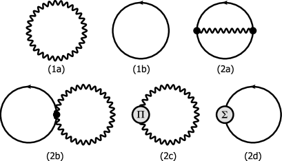
Figure 2: Diagrams contributing through NLO in HTLpt. The undulating lines are photon propagators and the solid lines are fermion propagators. A circle with a $\Pi$ indicates a photon self-energy insertion and a circle with a $\Sigma$ indicates a fermion self-energy insertion. All propagators and vertices shown are HTL-resummed propagators and vertices.

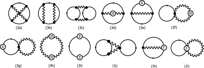
Figure 3: Diagrams contributing to NNLO in HTLpt which contribute through order $e^{5}$. The undulating lines are photon propagators and the solid lines are fermion propagators. A circle with a $\Pi$ indicates a photon self-energy insertion and a circle with a $\Sigma$ indicates a fermion self-energy insertion. The propagators are HTL-resummed propagators and the black dots indicate HTL-resummed vertices. The lettered vertices indicate that only the HTL correction is included.

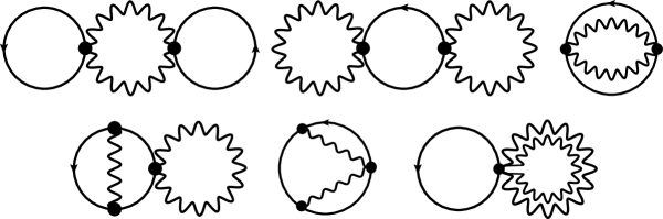
Figure 4: Diagrams contributing to NNLO in HTLpt which contribute beyond order $e^{5}$. The diagrams in the first line above first contribute at order $e^{8}$ and the second line at order $e^{6}$. The undulating lines are photon propagators and the solid lines are fermion propagators. All propagators and vertices shown are HTL-resummed propagators and vertices.

The thermodynamic potential at leading order in HTL perturbation theory for QED with $N_{f}$ massless electrons is

$$\Omega_{\rm LO}={\cal F}_{\rm 1a}+N_{f}{\cal F}_{\rm 1b}+\Delta_{0}{\cal E}_{0}\;.$$ (11)

Here, ${\cal F}_{1a}$ is the contribution from the photons

$$\!\!\!\!\!\!\!{\cal F}_{1a}\!\! = \!\!-{1\over 2}\hbox{$\sum$}\!\!\!\!\!\!\!\int_{P}\!\left\{(d-1)\log\left[-\Delta_{T}(P)\right]+\log\Delta_{L}(P)\right\}.$$ (12)

The transverse and longitudinal HTL propagators $\Delta_{T}(P)$ and $\Delta_{L}(P)$ are given in (51) and (52). The electron contribution is

$${\cal F}_{\rm 1b}=-\hbox{$\sum$}\!\!\!\!\!\!\!\int_{\{P\}}\log\det\left[P\!\!\!\!/-\Sigma(P)\right]\;.$$ (13)

The leading-order vacuum counterterm $\Delta_{0}{\cal E}_{0}$ is given by

$$\Delta_{0}{\cal E}_{0} = {1\over 128\pi^{2}\epsilon}m_{D}^{4}\;.$$ (14)

The thermodynamic potential at next-to-leading order (NLO) in HTL perturbation theory can be written as

$$\Omega_{\rm NLO} = \Omega_{\rm LO}+N_{f}\left({\cal F}_{\rm 2a}+{\cal F}_{\rm 2b}+{\cal F}_{\rm 2d}\right)+{\cal F}_{\rm 2c}+\Delta_{1}{\cal E}_{0}$$ (15)

$$+\Delta_{1}m_{D}^{2}{\partial\over\partial m_{D}^{2}}\Omega_{\rm LO}+\Delta_{1}m_{f}^{2}{\partial\over\partial m_{f}^{2}}\Omega_{\rm LO}\;,$$

where $\Delta_{1}{\cal E}_{0}$, $\Delta_{1}m_{D}^{2}$, and $\Delta_{1}m_{f}^{2}$ are the terms of order $\delta$ in the vacuum energy density and mass counterterms:

$$\Delta_{1}{\cal E}_{0} = -{1\over 64\pi^{2}\epsilon}m_{D}^{4}\;,$$ (16)

$$\Delta_{1}m_{D}^{2} = N_{f}{\alpha\over 3\pi\epsilon}m_{D}^{2}\;,$$ (17)

$$\Delta_{1}m_{f}^{2} = -{3\alpha\over 4\pi\epsilon}m_{f}^{2}\;.$$ (18)

The contributions from the two-loop diagrams with electron-photon three- and four-point vertices are

$${\cal F}_{\rm 2a} = {1\over 2}e^{2}\hbox{$\sum$}\!\!\!\!\!\!\!\int_{P\{Q\}}\mbox{Tr}\left[\Gamma^{\mu}(P,Q,R)S(Q)\Gamma^{\nu}(P,Q,R)S(R)\right]$$ (19)

$$\hskip 56.9055pt\times\Delta^{\mu\nu}(P)\;,$$

$${\cal F}_{\rm 2b} = {1\over 2}e^{2}\hbox{$\sum$}\!\!\!\!\!\!\!\int_{P\{Q\}}\mbox{Tr}\left[\Gamma^{\mu\nu}(P,-P,Q,Q)S(Q)\right]$$ (20)

$$\hskip 56.9055pt\times\Delta^{\mu\nu}(P)\;,$$

where $R=Q-P$.

The contribution from the HTL photon counterterm diagram with a single photon self-energy insertion is

$${\cal F}_{\rm 2c} = {1\over 2}\hbox{$\sum$}\!\!\!\!\!\!\!\int_{P}\Pi^{\mu\nu}(P)\Delta^{\mu\nu}(P)\;.$$ (21)

The contribution from the HTL electron counterterm diagram with a single electron self-energy insertion is

$${\cal F}_{\rm 2d} = -\hbox{$\sum$}\!\!\!\!\!\!\!\int_{\{P\}}\mbox{Tr}\left[\Sigma(P)S(P)\right]\;.$$ (22)

The role of the counterterm diagrams $\rm(2c)$ and $\rm(2d)$ is to avoid overcounting of diagrams when using effective propagators in $\rm(1a)$ and $\rm(1b)$. Similarly, the role of counterterm diagram $\rm(3k)$ is to avoid overcounting when using effective vertices in $(\rm 2a)$.

The thermodynamic potential at next-to-next-to-leading order (NNLO) in HTL perturbation theory can be written as

$$\Omega_{\rm NNLO} = \Omega_{\rm NLO}+N_{f}^{2}({\cal F}_{\rm 3c}+{\cal F}_{\rm 3j})+N_{f}({\cal F}_{\rm 3a}+{\cal F}_{\rm 3b}+{\cal F}_{\rm 3d}+{\cal F}_{\rm 3e}+{\cal F}_{\rm 3f}+{\cal F}_{\rm 3g}+{\cal F}_{\rm 3i}+{\cal F}_{\rm 3k}+{\cal F}_{\rm 3l})+{\cal F}_{\rm 3h}$$ (23)

$$+\Delta_{2}{\cal E}_{0}+\Delta_{2}m_{D}^{2}{\partial\over\partial m_{D}^{2}}\Omega_{\rm LO}+\Delta_{2}m_{f}^{2}{\partial\over\partial m_{f}^{2}}\Omega_{\rm LO}+\Delta_{1}m_{D}^{2}{\partial\over\partial m_{D}^{2}}\Omega_{\rm NLO}+\Delta_{1}m_{f}^{2}{\partial\over\partial m_{f}^{2}}\Omega_{\rm NLO}$$

$$+{1\over 2}\left({\partial^{2}\over(\partial m_{D}^{2})^{2}}\Omega_{\rm LO}\right)\left(\Delta_{1}m_{D}^{2}\right)^{2}+{1\over 2}\left({\partial^{2}\over(\partial m_{f}^{2})^{2}}\Omega_{\rm LO}\right)\left(\Delta_{1}m_{f}^{2}\right)^{2}+{F_{\rm 2a+2b}\over\alpha}\Delta_{1}\alpha\;.$$

where $\Delta_{2}{\cal E}_{0}$, $\Delta_{2}m_{D}^{2}$, $\Delta_{2}m_{f}^{2}$, and $\Delta_{1}\alpha$ are the terms of order $\delta^{2}$ in the vacuum energy density, mass and coupling constant counterterms:

$$\Delta_{2}{\cal E}_{0} = {1\over 128\pi^{2}\epsilon}m_{D}^{4}\;,$$ (24)

$$\Delta_{2}m_{D}^{2} = -N_{f}{\alpha\over 3\pi\epsilon}m_{D}^{2}\;,$$ (25)

$$\Delta_{2}m_{f}^{2} = {3\alpha\over 4\pi\epsilon}m_{f}^{2}\;.$$ (26)

The contributions from the three-loop diagrams are given by

$${\cal F}_{\rm 3a} = {1\over 4}e^{4}\hbox{$\sum$}\!\!\!\!\!\!\!\int_{P\{QR\}}{\rm Tr}\left[\Gamma^{\mu}(-P,Q-P,Q)S(Q)\Gamma^{\alpha}(Q-R,Q,R)S(R)\Gamma^{\nu}(P,R,R-P)\right.$$ (27)

$$\left.\times S(R-P)\Gamma^{\beta}(-Q+R,R-P,Q-P)S(Q-P)\right]\Delta^{\mu\nu}(P)\Delta^{\alpha\beta}(Q-R)\;,$$

$${\cal F}_{\rm 3b} = {1\over 2}e^{4}\hbox{$\sum$}\!\!\!\!\!\!\!\int_{P\{QR\}}{\rm Tr}\left[\Gamma^{\mu}(P,P+Q,Q)S(Q)\Gamma^{\beta}(-R+Q,Q,R)S(R)\Gamma^{\alpha}(R-Q,R,Q)\right.$$ (28)

$$\left.\times S(Q)\Gamma^{\nu}(-P,Q,P+Q)S(P+Q)\right]\Delta^{\mu\nu}(P)\Delta^{\alpha\beta}(R-Q)\;,$$

$${\cal F}_{\rm 3c} = -{1\over 4}e^{4}\hbox{$\sum$}\!\!\!\!\!\!\!\int_{P\{QR\}}{\rm Tr}\left[\Gamma^{\mu}(P,P+Q,Q)S(Q)\Gamma^{\beta}(-P,Q,P+Q)S(P+Q)\right]$$ (29)

$$\times{\rm Tr}\left[\Gamma^{\nu}(-P,R,P+R)S(P+R)\Gamma^{\alpha}(P,P+R,R)S(R)\right]\Delta^{\mu\nu}(P)\Delta^{\alpha\beta}(P)\;,$$

$${\cal F}_{\rm 3j} = -{1\over 2}e^{4}\hbox{$\sum$}\!\!\!\!\!\!\!\int_{P\{QR\}}{\rm Tr}\left[\Gamma^{\alpha\beta}(P,-P,R,R)S(R)\right]\Delta^{\alpha\mu}(P)\Delta^{\beta\nu}(P)$$ (30)

$$\times{\rm Tr}\left[\Gamma^{\mu}(P,P+Q,Q)S(Q)\Gamma^{\nu}(-P,Q,P+Q)S(P+Q)\right]\,.$$

The contributions from the two-loop diagrams with electron-photon three- and four-point vertices with an insertion of a photon self-energy

$${\cal F}_{\rm 3d} = -{1\over 2}e^{2}\hbox{$\sum$}\!\!\!\!\!\!\!\int_{P\{Q\}}\mbox{Tr}\left[\Gamma^{\mu}(P,Q,R)S(Q)\Gamma^{\nu}(P,Q,R)S(R)\right]$$ (31)

$$\times\Delta^{\mu\alpha}(P)\Pi^{\alpha\beta}(P)\Delta^{\beta\nu}(P)\;,$$

$${\cal F}_{\rm 3f} = -{1\over 2}e^{2}\hbox{$\sum$}\!\!\!\!\!\!\!\int_{P\{Q\}}\mbox{Tr}\left[\Gamma^{\mu\nu}(P,-P,Q,Q)S(Q)\right]$$ (32)

$$\hskip 28.45274pt\times\Delta^{\mu\alpha}(P)\Pi^{\alpha\beta}(P)\Delta^{\beta\nu}(P)\;,$$

where $R=Q-P$.

The contributions from the two-loop diagrams with the electron-photon three and four-point vertices with an insertion of an electron self-energy are

$${\cal F}_{\rm 3e} = -e^{2}\hbox{$\sum$}\!\!\!\!\!\!\!\int_{P\{Q\}}\Delta^{\alpha\beta}(P){\rm Tr}\left[\Gamma^{\alpha}(P,Q,R)S(Q)\right.$$ (33)

$$\left.\times\Sigma(Q)S(Q)\Gamma^{\beta}(P,Q,R)S(R)\right]\;,$$

$${\cal F}_{\rm 3g} = -{1\over 2}e^{2}\hbox{$\sum$}\!\!\!\!\!\!\!\int_{P\{Q\}}\Delta^{\mu\nu}(P)$$ (34)

$$\times{\rm Tr}\left[\Gamma^{\mu\nu}(P,-P,Q,Q)S(Q)\Sigma(Q)S(Q)\right]\;,$$

where $R=Q-P$.

The contribution from the HTL photon counterterm diagram with two photon self-energy insertions is

$${\cal F}_{3h} = -{1\over 4}\hbox{$\sum$}\!\!\!\!\!\!\!\int_{P}\Pi^{\mu\nu}(P)\Delta^{\nu\alpha}(P)\Pi^{\alpha\beta}(P)\Delta^{\beta\mu}(P)\;.$$ (35)

The contribution from HTL electron counterterm with two electron self-energy insertions is

$${\cal F}_{\rm 3i} = {1\over 2}\hbox{$\sum$}\!\!\!\!\!\!\!\int_{\{P\}}{\rm Tr}\left[S(P)\Sigma(P)S(P)\Sigma(P)\right]\;.$$ (36)

The remaining three-loop diagrams involving HTL corrected vertex terms are given by

$${\cal F}_{\rm 3k} = e^{2}m_{f}^{2}\hbox{$\sum$}\!\!\!\!\!\!\!\int_{P\{Q\}}\!\!\!\!\!\!\mbox{Tr}\!\left[\tilde{\cal T}^{\mu}(P,Q,R)S(Q)\Gamma^{\nu}(P,Q,R)S(R)\right]$$ (37)

$$\hskip 56.9055pt\times\Delta^{\mu\nu}(P)\;,$$

$${\cal F}_{\rm 3l} = -{1\over 2}e^{2}\hbox{$\sum$}\!\!\!\!\!\!\!\int_{P\{Q\}}\mbox{Tr}\left[\Gamma^{\mu\nu}(P,-P,Q,Q)S(Q)\right]$$ (38)

$$\hskip 56.9055pt\times\Delta^{\mu\nu}(P)\;,$$

where $\tilde{\cal T}^{\mu}$ is the HTL correction term given in Eq. (43). Note also that diagram $\rm(3l)$ is the same as $\rm(2b)$ since there is no tree-level electron-photon four-vertex.

In the remainder of the paper, we work in Landau gauge ($\xi=0$), but we emphasize that the HTL perturbation theory method of reorganization is gauge-fixing independent to all orders in $\delta$ (loop expansion) by construction.

IV Expansion in the mass parameters

In the papers htl2 ; aps1 , the free energy was reduced to scalar sum-integrals. It was clear that evaluating these scalar sum-integrals exactly was intractable and the sum-integrals were calculated approximately by expanding them in powers of $m_{D}/T$ and $m_{f}/T$. We will follow the same strategy in this paper and carry out the expansion to high enough order to include all terms through order $e^{5}$ if $m_{D}$ and $m_{f}$ are taken to be of order $e$. The NLO approximation will be perturbatively accurate to order $e^{3}$ and the NNLO approximation accurate to order $e^{5}$.

The free energy can be divided into contributions from hard and soft momenta. In the one-loop diagrams, the contributions are either hard $(h)$ or soft $(s)$, while at the two-loop level, there are hard-hard $(hh)$ and hard-soft $(hs)$ contributions. There are no soft-soft $(ss)$ contributions since one of the loop momenta is fermionic and always hard. At three loops there are hard-hard-hard $(hhh)$, hard-hard-soft $(hhs)$, and hard-soft-soft $(hss)$ contributions. There are no soft-soft-soft $(sss)$ contributions, again due to the hard fermionic lines.

In the process of the calculation we will see that there are many cancellations between the lower-order HTL-improved diagrams and the higher-order HTL-improved counterterm diagrams. This is by construction and is part of the systematic way in which HTLpt converges to the known perturbative expansion. For example, one can see that diagrams (2c) and (3h) subtract out the modification of the hard gluon propagator due to the HTL-improvement of the propagator in diagram (1a). Likewise, one expects cancellations to occur between diagrams (1b), (2d) and (3i); (2a), (3d), (3e) and (3k); and (2b), (3f), (3g), and (3l). Below we will explicitly demonstrate how these cancellations occur.

IV.1 One-loop sum-integrals

IV.1.1 Hard contribution

For hard momenta, the self-energies are suppressed by $m_{D}/T$ and $m_{f}/T$ relative to the inverse free propagators, so we can expand in powers of $\Pi_{T}(P)$, $\Pi_{L}(P)$, and $\Sigma(P)$.

For the one-loop graph $\rm(1a)$, we need to expand to second order in $m^{2}_{D}$:

$${\cal F}_{\rm 1a}^{(h)} = {1\over 2}(d-1)\hbox{$\sum$}\!\!\!\!\!\!\!\int_{P}\log\left(P^{2}\right)+{1\over 2}m_{D}^{2}\hbox{$\sum$}\!\!\!\!\!\!\!\int_{P}{1\over P^{2}}-{1\over 4(d-1)}m_{D}^{4}\hbox{$\sum$}\!\!\!\!\!\!\!\int_{P}\left[{1\over P^{4}}-2{1\over p^{2}P^{2}}-2d{1\over p^{4}}{\cal T}_{P}+2{1\over p^{2}P^{2}}{\cal T}_{P}+d{1\over p^{4}}\left({\cal T}_{P}\right)^{2}\right]$$ (39)

$$= -{\pi^{2}\over 45}T^{4}+{1\over 24}\left[1+\left(2+2{\zeta^{\prime}(-1)\over\zeta(-1)}\right)\epsilon\right]\left({\mu\over 4\pi T}\right)^{2\epsilon}m_{D}^{2}T^{2}-{1\over 128\pi^{2}}\left({1\over\epsilon}-7+2\gamma+{2\pi^{2}\over 3}\right)\left({\mu\over 4\pi T}\right)^{2\epsilon}m_{D}^{4}\,.$$

The one-loop graph with a photon self-energy insertion $(\rm 2c$) has an explicit factor of $m_{D}^{2}$ and so we need only to expand the sum-integral to first order in $m_{D}^{2}$:

$${\cal F}_{\rm 2c}^{(h)}\!\! = \!\!-{1\over 2}m_{D}^{2}\hbox{$\sum$}\!\!\!\!\!\!\!\int_{P}{1\over P^{2}}+{1\over 2(d-1)}m_{D}^{4}\hbox{$\sum$}\!\!\!\!\!\!\!\int_{P}\left[{1\over P^{4}}-2{1\over p^{2}P^{2}}-2d{1\over p^{4}}{\cal T}_{P}+2{1\over p^{2}P^{2}}{\cal T}_{P}+d{1\over p^{4}}\left({\cal T}_{P}\right)^{2}\right]\;,$$ (40)

$$= \!\!-{1\over 24}\left[1+\left(2+2{\zeta^{\prime}(-1)\over\zeta(-1)}\right)\epsilon\right]\left({\mu\over 4\pi T}\right)^{2\epsilon}m_{D}^{2}T^{2}+{1\over 64\pi^{2}}\left({1\over\epsilon}-7+2\gamma+{2\pi^{2}\over 3}\right)\left({\mu\over 4\pi T}\right)^{2\epsilon}m_{D}^{4}\,.$$

The one-loop graph with two photon self-energy insertions ($\rm 3h$) must be expanded to zeroth order in $m_{D}^{2}$

$${\cal F}_{\rm 3h}^{(h)} = -{1\over 4(d-1)}m_{D}^{4}\hbox{$\sum$}\!\!\!\!\!\!\!\int_{P}\left[{1\over P^{4}}-2{1\over p^{2}P^{2}}-2d{1\over p^{4}}{\cal T}_{P}+2{1\over p^{2}P^{2}}{\cal T}_{P}+d{1\over p^{4}}\left({\cal T}_{P}\right)^{2}\right]\;.$$ (41)

$$= -{1\over 128\pi^{2}}\left({1\over\epsilon}-7+2\gamma+{2\pi^{2}\over 3}\right)\left({\mu\over 4\pi T}\right)^{2\epsilon}m_{D}^{4}\,.$$

The sum of Eqs. (39)-(41) is very simple:

$${\cal F}_{\rm 1a+2c+3h}^{(h)} = {1\over 2}(d-1)\hbox{$\sum$}\!\!\!\!\!\!\!\int_{P}\log\left(P^{2}\right)$$ (42)

$$= -{\pi^{2}\over 45}T^{4}\;.$$

This is the free energy of an ideal gas of photons.

The one-loop graph $(1b)$ needs to expanded to second order in $m^{2}_{f}$:

$${\cal F}_{\rm 1b}^{(h)} = -2\hbox{$\sum$}\!\!\!\!\!\!\!\int_{\{P\}}\log P^{2}-4m_{f}^{2}\hbox{$\sum$}\!\!\!\!\!\!\!\int_{\{P\}}{1\over P^{2}}+2m_{f}^{4}\hbox{$\sum$}\!\!\!\!\!\!\!\int_{\{P\}}\left[{2\over P^{4}}-{1\over p^{2}P^{2}}+{2\over p^{2}P^{2}}{\cal T}_{P}-{1\over p^{2}P_{0}^{2}}\left({\cal T}_{P}\right)^{2}\right]$$ (43)

$$= -{7\pi^{2}\over 180}T^{4}+{1\over 6}\left[1+\left(2-2\log 2+2{\zeta^{\prime}(-1)\over\zeta(-1)}\right)\epsilon\right]\left({\mu\over 4\pi T}\right)^{2\epsilon}m_{f}^{2}T^{2}+{1\over 12\pi^{2}}\left(\pi^{2}-6\right)m_{f}^{4}\,.$$

The one-loop fermion loop with a fermion self-energy insertion $\rm(2d)$ must be expanded to first order in $m_{f}^{2}$,

$${\cal F}_{\rm 2d}^{(h)} = 4m_{f}^{2}\hbox{$\sum$}\!\!\!\!\!\!\!\int_{\{P\}}{1\over P^{2}}-4m_{f}^{4}\hbox{$\sum$}\!\!\!\!\!\!\!\int_{\{P\}}\left[{2\over P^{4}}-{1\over p^{2}P^{2}}+{2\over p^{2}P^{2}}{\cal T}_{P}-{1\over p^{2}P_{0}^{2}}\left({\cal T}_{P}\right)^{2}\right]$$ (44)

$$= -{1\over 6}\left[1+\left(2-2\log 2+2{\zeta^{\prime}(-1)\over\zeta(-1)}\right)\epsilon\right]\left({\mu\over 4\pi T}\right)^{2\epsilon}m_{f}^{2}T^{2}-{1\over 6\pi^{2}}\left(\pi^{2}-6\right)m_{f}^{4}\,.$$

The one-loop fermion loop with two self-energy insertions $\rm(3i)$ must be expanded to zeroth order in $m_{f}^{2}$:

$${\cal F}_{\rm 3i}^{(h)} = 2m_{f}^{4}\hbox{$\sum$}\!\!\!\!\!\!\!\int_{\{P\}}\left[{2\over P^{4}}-{1\over p^{2}P^{2}}+{2\over p^{2}P^{2}}{\cal T}_{P}-{1\over p^{2}P_{0}^{2}}\left({\cal T}_{P}\right)^{2}\right]$$ (45)

$$= {1\over 12\pi^{2}}\left(\pi^{2}-6\right)m_{f}^{4}\,.$$

The sum of Eqs. (43)-(45) is particularly simple:

$${\cal F}_{\rm 1b+2d+3i}^{(h)} = -2\hbox{$\sum$}\!\!\!\!\!\!\!\int_{\{P\}}\log P^{2}$$ (46)

$$= -{7\pi^{2}\over 180}T^{4}\;.$$

This is the free energy of an ideal gas of a single massless fermion.

IV.1.2 Soft contribution

The soft contributions in the diagrams $(1a)$, $(2c)$, and $(3h)$ arise from the $P_{0}=0$ term in the sum-integral. At soft momentum $P=(0,{\bf p})$, the HTL self-energy functions reduce to $\Pi_{T}(P)=0$ and $\Pi_{L}(P)=m_{D}^{2}$. The transverse term vanishes in dimensional regularization because there is no momentum scale in the integral over ${\bf p}$. Thus the soft contributions come from the longitudinal term only and read

$${\cal F}^{(s)}_{\rm 1a} = {1\over 2}T\int_{p}\log\left(p^{2}+m_{D}^{2}\right)$$

$$= -{m_{D}^{3}T\over 12\pi}\left({\mu\over 2m}\right)^{2\epsilon}\left[1+{8\over 3}\epsilon\right]\;,$$

$${\cal F}^{(s)}_{\rm 2c} = -{1\over 2}m_{D}^{2}T\int_{p}{1\over p^{2}+m_{D}^{2}}$$

$$= {m^{3}_{D}T\over 8\pi}\left({\mu\over 2m_{D}}\right)^{2\epsilon}\left[1+2\epsilon\right]\;,$$

$${\cal F}^{(s)}_{\rm 3h} = -{1\over 4}m_{D}^{4}T\int_{p}{1\over(p^{2}+m_{D}^{2})^{2}}$$ (49)

$$= -{m^{3}_{D}T\over 32\pi}\;.$$

Note that we have kept the terms through order $\epsilon$ in Eqs. (LABEL:count11) and (IV.1.2) as they are required in the calculation of the counterterms. There is no soft contribution from the leading-order fermion term (13) or from the HTL counterterms (22) and (36).

IV.2 Two-loop sum-integrals

For hard momenta, the self-energies are suppressed by $m_{D}/T$ and $m_{f}/T$ relative to the inverse free propagators, so we can expand in powers of $\Pi_{T}$, $\Pi_{L}$, and $\Sigma$.

IV.2.1 (hh) contribution

The $(hh)$ contribution from (19) and (20) was calculated in Ref. aps1 and reads

$${\cal F}_{\rm 2a+2b}^{(hh)} = (d-1)e^{2}\left[\hbox{$\sum$}\!\!\!\!\!\!\!\int_{\{PQ\}}{1\over P^{2}Q^{2}}-\hbox{$\sum$}\!\!\!\!\!\!\!\int_{P\{Q\}}{2\over P^{2}Q^{2}}\right]+2m_{D}^{2}e^{2}\hbox{$\sum$}\!\!\!\!\!\!\!\int_{P\{Q\}}\left[{1\over p^{2}P^{2}Q^{2}}{\cal T}_{P}+{1\over(P^{2})^{2}Q^{2}}-{d-2\over d-1}{1\over p^{2}P^{2}Q^{2}}\right]$$

$$+m_{D}^{2}e^{2}\hbox{$\sum$}\!\!\!\!\!\!\!\int_{\{PQ\}}\left[{d+1\over d-1}{1\over P^{2}Q^{2}r^{2}}-{4d\over d-1}{q^{2}\over P^{2}Q^{2}r^{4}}-{2d\over d-1}{P\!\cdot\!Q\over P^{2}Q^{2}r^{4}}\right]{\cal T}_{R}$$

$$+m_{D}^{2}e^{2}\hbox{$\sum$}\!\!\!\!\!\!\!\int_{\{PQ\}}\left[{3-d\over d-1}{1\over P^{2}Q^{2}R^{2}}+{2d\over d-1}{P\!\cdot\!Q\over P^{2}Q^{2}r^{4}}-{d+2\over d-1}{1\over P^{2}Q^{2}r^{2}}+{4d\over d-1}{q^{2}\over P^{2}Q^{2}r^{4}}-{4\over d-1}{q^{2}\over P^{2}Q^{2}r^{2}R^{2}}\right]$$

$$+2m_{f}^{2}e^{2}(d-1)\hbox{$\sum$}\!\!\!\!\!\!\!\int_{\{PQ\}}\left[{1\over P^{2}Q_{0}^{2}Q^{2}}+{p^{2}-r^{2}\over P^{2}q^{2}Q_{0}^{2}R^{2}}\right]{\cal T}_{Q}+2m_{f}^{2}e^{2}(d-1)\hbox{$\sum$}\!\!\!\!\!\!\!\int_{P\{Q\}}\left[{2\over P^{2}(Q^{2})^{2}}-{1\over P^{2}Q_{0}^{2}Q^{2}}{\cal T}_{Q}\right]$$

$$+2m_{f}^{2}e^{2}(d-1)\hbox{$\sum$}\!\!\!\!\!\!\!\int_{\{PQ\}}\left[{d+3\over d-1}{1\over P^{2}Q^{2}R^{2}}-{2\over P^{2}(Q^{2})^{2}}+{r^{2}-p^{2}\over q^{2}P^{2}Q^{2}R^{2}}\right]$$

$$= {5\pi^{2}\over 72}{\alpha\over\pi}T^{4}\left[1+\left(3-{12\over 5}\log 2+4{\zeta^{\prime}(-1)\over\zeta(-1)}\right)\epsilon\right]\left({\mu\over 4\pi T}\right)^{4\epsilon}$$

$$-{1\over 72}\left[{1\over\epsilon}\;+\;1.30107\right]{\alpha\over\pi}\left({\mu\over 4\pi T}\right)^{4\epsilon}m_{D}^{2}T^{2}+{1\over 8}\left[{1\over\epsilon}\;+\;8.97544\right]{\alpha\over\pi}\left({\mu\over 4\pi T}\right)^{4\epsilon}m_{f}^{2}T^{2}\;.$$

Consider next the $(hh)$ contribution from (31) and (32). The easiest way to calculate this term, is to expand the two-loop diagrams $\rm(2a)$ and $(\rm 2b)$ to first order in $m_{D}^{2}$. This yields

$${\cal F}_{\rm 3d+3f}^{(hh)} = -2m_{D}^{2}e^{2}\hbox{$\sum$}\!\!\!\!\!\!\!\int_{P\{Q\}}\left[{1\over p^{2}P^{2}Q^{2}}{\cal T}_{P}+{1\over(P^{2})^{2}Q^{2}}-{d-2\over d-1}{1\over p^{2}P^{2}Q^{2}}\right]$$ (51)

$$-m_{D}^{2}e^{2}\hbox{$\sum$}\!\!\!\!\!\!\!\int_{\{PQ\}}\left[{d+1\over d-1}{1\over P^{2}Q^{2}r^{2}}-{4d\over d-1}{q^{2}\over P^{2}Q^{2}r^{4}}-{2d\over d-1}{P\!\cdot\!Q\over P^{2}Q^{2}r^{4}}\right]{\cal T}_{R}$$

$$-m_{D}^{2}e^{2}\hbox{$\sum$}\!\!\!\!\!\!\!\int_{\{PQ\}}\left[{3-d\over d-1}{1\over P^{2}Q^{2}R^{2}}+{2d\over d-1}{P\!\cdot\!Q\over P^{2}Q^{2}r^{4}}-{d+2\over d-1}{1\over P^{2}Q^{2}r^{2}}+{4d\over d-1}{q^{2}\over P^{2}Q^{2}r^{4}}-{4\over d-1}{q^{2}\over P^{2}Q^{2}r^{2}R^{2}}\right]$$

$$= {1\over 72}\left[{1\over\epsilon}\;+\;1.30107\right]{\alpha\over\pi}\left({\mu\over 4\pi T}\right)^{4\epsilon}m_{D}^{2}T^{2}\;.$$

We also need the $(hh)$ contributions from the diagrams $(\rm 3e)$, $(\rm 3g)$, $(\rm 3k)$, and $(\rm 3l)$ The first two diagrams are given by (33),  (34), while the last remaining ones are given by  (37) and (38). The easiest way to calculate these contributions is to expand the two-loop diagrams $\rm(2a)$ and $(\rm 2b)$ to first order in $m_{f}^{2}$. This yields

$${\cal F}_{\rm 3e+3g+3k+3l}^{(hh)} = -2m_{f}^{2}e^{2}(d-1)\hbox{$\sum$}\!\!\!\!\!\!\!\int_{\{PQ\}}\left[{1\over P^{2}Q_{0}^{2}Q^{2}}+{p^{2}-r^{2}\over P^{2}q^{2}Q_{0}^{2}R^{2}}\right]{\cal T}_{Q}-2m_{f}^{2}e^{2}(d-1)\hbox{$\sum$}\!\!\!\!\!\!\!\int_{P\{Q\}}\left[{2\over P^{2}(Q^{2})^{2}}-{1\over P^{2}Q_{0}^{2}Q^{2}}{\cal T}_{Q}\right]$$ (52)

$$-2m_{f}^{2}e^{2}(d-1)\hbox{$\sum$}\!\!\!\!\!\!\!\int_{\{PQ\}}\left[{d+3\over d-1}{1\over P^{2}Q^{2}R^{2}}-{2\over P^{2}(Q^{2})^{2}}+{r^{2}-p^{2}\over q^{2}P^{2}Q^{2}R^{2}}\right]$$

$$= -{1\over 8}\left[{1\over\epsilon}\;+\;8.97544\right]{\alpha\over\pi}\left({\mu\over 4\pi T}\right)^{4\epsilon}m_{f}^{2}T^{2}\;.$$

The sum of the terms in (LABEL:33)–(52) is very simple

$${\cal F}_{\rm 2a+2b+3d+3e+3f+3g+3k+3l}^{(hh)} = (d-1)e^{2}\left[\hbox{$\sum$}\!\!\!\!\!\!\!\int_{\{PQ\}}{1\over P^{2}Q^{2}}-\hbox{$\sum$}\!\!\!\!\!\!\!\int_{P\{Q\}}{2\over P^{2}Q^{2}}\right]$$ (53)

$$= {5\pi^{2}\over 72}{\alpha\over\pi}T^{4}\,.$$

This is the two-loop contribution from the perturbative expansion of the free energy in QED.

IV.2.2 (hs) contribution

In the $(hs)$ region, the momentum $P$ is soft. The momenta $Q$ and $R$ are always hard. The function that multiplies the soft propagator $\Delta_{T}(0,{\bf p})$, $\Delta_{L}(0,{\bf p})$, or $\Delta_{X}(0,{\bf p})$ can be expanded in powers of the soft momentum ${\bf p}$. The soft propagators $\Delta_{T}(0,{\bf p})$, $\Delta_{L}(0,{\bf p})$, and $\Delta_{X}(0,{\bf p})$ are defined in Eqs. (21), (22) and (27), respectively. In the case of $\Delta_{T}(0,{\bf p})$, the resulting integrals over ${\bf p}$ have no scale and they vanish in dimensional regularization. The integration measure $\int_{\bf p}$ scales like $m_{D}^{3}$, the soft propagators $\Delta_{L}(0,{\bf p})$ and $\Delta_{X}(0,{\bf p})$ scale like $1/m_{D}^{2}$, and every power of $p$ in the numerator scales like $m_{D}$.

The terms that contribute through order $e^{2}m_{D}^{3}T$ and $e^{2}m_{f}^{2}m_{D}T$ from  (19) and (20) were calculated in Ref. aps1 and read

$${\cal F}_{2a+2b}^{(hs)} = 2e^{2}T\int_{p}{1\over p^{2}+m^{2}_{D}}\hbox{$\sum$}\!\!\!\!\!\!\!\int_{\{Q\}}\left[{1\over Q^{2}}-{2q^{2}\over Q^{4}}\right]+2m_{D}^{2}e^{2}T\int_{p}{1\over p^{2}+m_{D}^{2}}\hbox{$\sum$}\!\!\!\!\!\!\!\int_{\{Q\}}\left[{1\over Q^{4}}-{2\over d}(3+d){q^{2}\over Q^{6}}+{8\over d}{q^{4}\over Q^{8}}\right]$$ (54)

$$-4m_{f}^{2}e^{2}T\int_{p}{1\over p^{2}+m_{D}^{2}}\hbox{$\sum$}\!\!\!\!\!\!\!\int_{\{Q\}}\left[{3\over Q^{4}}-{4q^{2}\over Q^{6}}-{4\over Q^{4}}{\cal T}_{Q}-{2\over Q^{2}}\bigg{\langle}{1\over(Q\!\cdot\!Y)^{2}}\bigg{\rangle}_{\!\!\bf\hat{y}}\right]$$

$$= -{1\over 6}\alpha m_{D}T^{3}\left[1+\left(3-2\log 2+2{\zeta^{\prime}(-1)\over\zeta(-1)}\right)\epsilon\right]\left({\mu\over 4\pi T}\right)^{2\epsilon}\left({\mu\over 2m_{D}}\right)^{2\epsilon}$$

$$+{\alpha\over 24\pi^{2}}\left[{1\over\epsilon}+\left(1+2\gamma+4\log 2\right)\right]\left({\mu\over 4\pi T}\right)^{2\epsilon}\left({\mu\over 2m_{D}}\right)^{2\epsilon}m_{D}^{3}T-{\alpha\over 2\pi^{2}}m_{f}^{2}m_{D}T\;.$$

The $(hs)$ contribution from  (31) and (32) can again be calculated from the diagrams $\rm(2a)$ and $(\rm 2b)$ by Taylor expanding their contribution to first order in $m_{D}^{2}$. This yields

$${\cal F}_{\rm 3d+3f}^{(hs)} = 2m_{D}^{2}e^{2}T\int_{p}{1\over(p^{2}+m_{D}^{2})^{2}}\hbox{$\sum$}\!\!\!\!\!\!\!\int_{\{Q\}}\left[{1\over Q^{2}}-{2q^{2}\over Q^{4}}\right]-2m_{D}^{2}e^{2}T\int_{p}{p^{2}\over(p^{2}+m^{2}_{D})^{2}}\hbox{$\sum$}\!\!\!\!\!\!\!\int_{\{Q\}}\left[{1\over Q^{4}}-{2\over d}(3+d){q^{2}\over Q^{6}}+{8\over d}{q^{4}\over Q^{8}}\right]$$ (55)

$$-4m_{D}^{2}m_{f}^{2}e^{2}T\int_{p}{1\over(p^{2}+m_{D}^{2})^{2}}\hbox{$\sum$}\!\!\!\!\!\!\!\int_{\{Q\}}\left[{3\over Q^{4}}-{4q^{2}\over Q^{6}}-{4\over Q^{4}}{\cal T}_{Q}-{2\over Q^{2}}\bigg{\langle}{1\over(Q\!\cdot\!Y)^{2}}\bigg{\rangle}_{\!\!\bf\hat{y}}\right]$$

$$= {1\over 12}\alpha m_{D}T^{3}-{\alpha\over 16\pi^{2}}\left[{1\over\epsilon}+\left({1\over 3}+2\gamma+4\log 2\right)\right]\left({\mu\over 4\pi T}\right)^{2\epsilon}\left({\mu\over 2m_{D}}\right)^{2\epsilon}m_{D}^{3}T+{\alpha\over 4\pi^{2}}m_{f}^{2}m_{D}T\;.$$

We also need the $(hs)$ contributions from the diagrams $(\rm 3e)$, $(\rm 3g)$, $(\rm 3k)$, and $(\rm 3l)$ Again we calculate their contributions by expanding the two-loop diagrams $\rm(2a)$ and $(\rm 2b)$ to first order in $m_{f}^{2}$. This yields

$${\cal F}_{3e+3g+3k+3l}^{(hs)} = 4m_{f}^{2}e^{2}T\int_{p}{1\over p^{2}+m_{D}^{2}}\hbox{$\sum$}\!\!\!\!\!\!\!\int_{\{Q\}}\left[{3\over Q^{4}}-{4q^{2}\over Q^{6}}-{4\over Q^{4}}{\cal T}_{Q}-{2\over Q^{2}}\bigg{\langle}{1\over(Q\!\cdot\!Y)^{2}}\bigg{\rangle}_{\!\!\bf\hat{y}}\right]$$ (56)

$$= {\alpha\over 2\pi^{2}}m_{f}^{2}m_{D}T\;.$$

IV.2.3 (ss) contribution

There are no contributions from the $(ss)$ sector since fermionic momenta are always hard.

IV.3 Three-loop sum-integrals

IV.3.1 (hhh) contribution

If all three loop momenta are hard, we can expand the propagators in powers of $\Pi_{\mu\nu}(P)$ and $\Sigma(P)$. Through order $e^{5}$, we can use bare propagators and vertices. The diagrams $\rm(3a)$, $\rm(3b)$, and $\rm(3c)$ were calculated in Refs. qed4 ; AZ-95 and their contribution is

$${\cal F}^{(hhh)}_{\rm 3a+3b+3c} = {1\over 2}(d-1)(d-5)e^{4}\hbox{$\sum$}\!\!\!\!\!\!\!\int_{\{PQR\}}{1\over P^{2}Q^{2}R^{2}(P+Q+R)^{2}}-(d-1)(d-3)e^{4}\hbox{$\sum$}\!\!\!\!\!\!\!\int_{PQ\{R\}}{1\over P^{2}Q^{2}R^{2}(P+Q+R)^{2}}$$ (57)

$$+(d-1)^{2}e^{4}\hbox{$\sum$}\!\!\!\!\!\!\!\int_{\{P\}}{1\over P^{4}}\left[\hbox{$\sum$}\!\!\!\!\!\!\!\int_{Q}{1\over Q^{2}}-\hbox{$\sum$}\!\!\!\!\!\!\!\int_{\{Q\}}{1\over Q^{2}}\right]^{2}+(d-1)^{2}e^{4}\hbox{$\sum$}\!\!\!\!\!\!\!\int_{PQ\{R\}}{1\over P^{2}Q^{2}R^{2}(P+Q+R)^{2}}$$

$$-2(d-1)^{2}e^{4}\hbox{$\sum$}\!\!\!\!\!\!\!\int_{\{P\}QR}{Q\!\cdot\!R\over P^{2}Q^{2}R^{2}(P+Q)^{2}(P+R)^{2}}-4e^{4}(d-3)\hbox{$\sum$}\!\!\!\!\!\!\!\int_{P\{QR\}}{1\over P^{4}Q^{2}R^{2}}$$

$$-(d-3)e^{4}\hbox{$\sum$}\!\!\!\!\!\!\!\int_{\{PQR\}}{1\over P^{2}Q^{2}R^{2}(P+Q+R)^{2}}-16e^{4}\hbox{$\sum$}\!\!\!\!\!\!\!\int_{P\{QR\}}{(Q\!\cdot\!R)^{2}\over P^{4}Q^{2}R^{2}(P+Q)^{2}(P+R)^{2}}\;.$$

Using the expression for the sum-integrals in the Appendix, we obtain

$${\cal F}_{\rm N_{f}(3a+3b)+N_{f}^{2}3c}^{(hhh)} = -N_{f}^{2}{5\pi^{2}\over 216}\left({\alpha\over\pi}\right)^{2}T^{4}\left({\mu\over 4\pi T}\right)^{6\epsilon}\left[{1\over\epsilon}+{31\over 10}+{6\over 5}\gamma-{192\over 25}\log 2\right.\left.+{28\over 5}{\zeta^{\prime}(-1)\over\zeta(-1)}-{4\over 5}{\zeta^{\prime}(-3)\over\zeta(-3)}\right]$$ (58)

$$+N_{f}{\pi^{2}\over 192}\left({\alpha\over\pi}\right)^{2}T^{4}\left[35-32\log 2\right]\;.$$

IV.3.2 (hhs) contribution

The diagrams $\rm(3a)$ and $\rm(3b)$ are both infrared finite in the limit $m_{D}\rightarrow 0$. This implies that the $e^{5}$ contribution is given by using a dressed longitudinal propagator and bare vertices. The ring diagram $\rm(3c)$ is infrared divergent in that limit. The contribution through $e^{5}$ is obtained by expanding in powers of self-energies and vertices. Finally, the diagram $\rm(3j)$ also gives a contribution of order $e^{5}$. Since the electron-photon four-vertex is already of order $e^{2}m_{f}^{2}$, we can use a dressed longitudinal propagator and bare fermion propagators as well as bare electron-photon three-vertices. Note that both $(\rm 3c)$ and $(\rm 3j)$ are proportional to $N_{f}^{2}$ and so it is more convenient to calculate their sum. One finds

$${\cal F}_{\rm 3a}^{(hhs)} = 2(d-1)(d-3)e^{4}T\int_{p}{1\over p^{2}+m_{D}^{2}}\hbox{$\sum$}\!\!\!\!\!\!\!\int_{\{Q\}}{1\over Q^{4}}\left[\hbox{$\sum$}\!\!\!\!\!\!\!\int_{R}{1\over R^{2}}-\hbox{$\sum$}\!\!\!\!\!\!\!\int_{\{R\}}{1\over R^{2}}\right]$$ (59)

$$+8(d-1)e^{4}T\int_{p}{1\over p^{2}+m_{D}^{2}}\hbox{$\sum$}\!\!\!\!\!\!\!\int_{Q\{R\}}{q_{0}r_{0}\over Q^{2}R^{4}(Q+R)^{2}}\;,$$

$${\cal F}_{\rm 3b}^{(hhs)} = -8(d-1)e^{4}T\int_{p}{1\over p^{2}+m_{D}^{2}}\hbox{$\sum$}\!\!\!\!\!\!\!\int_{Q\{R\}}{q_{0}r_{0}\over Q^{2}R^{4}(Q+R)^{2}}\;,$$ (60)

$${\cal F}_{3c+3j}^{(hhs)} = -4e^{4}T\int_{p}{1\over(p^{2}+m_{D}^{2})^{2}}\left[\hbox{$\sum$}\!\!\!\!\!\!\!\int_{\{Q\}}{1\over Q^{2}}-{2q^{2}\over Q^{4}}\right]^{2}$$ (61)

$$+8e^{4}T\int_{p}{p^{2}\over(p^{2}+m_{D}^{2})^{2}}\hbox{$\sum$}\!\!\!\!\!\!\!\int_{\{Q\}}\left[{1\over Q^{2}}-{2q^{2}\over Q^{4}}\right]\hbox{$\sum$}\!\!\!\!\!\!\!\int_{\{R\}}\left[{1\over R^{4}}-{2\over d}(3+d){r^{2}\over R^{6}}+{8\over d}{r^{4}\over R^{8}}\right]$$

$$-16m_{f}^{2}e^{4}T\int_{p}{1\over(p^{2}+m_{D}^{2})^{2}}\hbox{$\sum$}\!\!\!\!\!\!\!\int_{\{Q\}}\left[{1\over Q^{2}}-{2q^{2}\over Q^{4}}\right]\hbox{$\sum$}\!\!\!\!\!\!\!\int_{\{R\}}\left[{3\over R^{4}}-{4r^{2}\over R^{6}}-{4\over R^{4}}{\cal T}_{R}-{2\over R^{2}}\bigg{\langle}{1\over(R\!\cdot\!Y)^{2}}\bigg{\rangle}_{\!\!\bf\hat{y}}\right]\;.$$

Using the expressions for the integrals and sum-integrals listed in the Appendix, we obtain

$${\cal F}_{\rm N_{f}(3a+3b)+N_{f}^{2}(3c+3j)}^{(hhs)} = -N_{f}^{2}{\pi\alpha^{2}T^{5}\over 18m_{D}}+N_{f}^{2}{\alpha^{2}m_{D}T^{3}\over 12\pi}\left[{1\over\epsilon}+{4\over 3}+2\gamma+2\log 2+2{\zeta^{\prime}(-1)\over\zeta(-1)}\right]\left({\mu\over 4\pi T}\right)^{4\epsilon}\left({\mu\over 2m_{D}}\right)^{2\epsilon}$$

$$\hskip 142.26378pt+N_{f}{\alpha^{2}m_{D}T^{3}\over 4\pi}\ -N_{f}^{2}{\alpha^{2}\over 3\pi m_{D}}m_{f}^{2}T^{3}\;.$$

IV.3.3 (hss) contribution

The $(hss)$ modes first start to contribute at order $e^{6}$, and therefore at our truncation order the $(hss)$ contributions vanish.

IV.3.4 (sss) contribution

There are no contributions from the $(sss)$ sector since fermionic momenta are always hard.

V The Thermodynamic Potential

In this section we present the final renormalized thermodynamic potential explicitly through order $\delta^{2}$, aka NNLO. The final NNLO expression is completely analytic; however, there are some numerically determined constants which remain in the final expressions at NLO.

V.1 Leading order

The complete expression for the leading order thermodynamic potential is given by the sum of Eqs. (39), (43), and (LABEL:count11) plus the leading vacuum energy counterterm (14):

$$\Omega_{\rm LO} = -{\pi^{2}T^{4}\over 45}\left\{1+{7\over 4}N_{f}-{15\over 2}\hat{m}_{D}^{2}-30N_{f}\hat{m}_{f}^{2}+30\hat{m}_{D}^{3}+{45\over 4}\left(\log{\hat{\mu}\over 2}-{7\over 2}+\gamma+{\pi^{2}\over 3}\right)\hat{m}_{D}^{4}-60N_{f}\left(\pi^{2}-6\right)\hat{m}_{f}^{4}\right\}\;.$$

where $\hat{m}_{D}$, $\hat{m}_{f}$, and $\hat{\mu}$ are dimensionless variables:

$$\hat{m}_{D} = {m_{D}\over 2\pi T}\;,$$ (64)

$$\hat{m}_{f} = {m_{f}\over 2\pi T}\;,$$ (65)

$$\hat{\mu} = {\mu\over 2\pi T}\;.$$ (66)

V.2 Next-to-leading order

The renormalization contributions at first order in $\delta$ are

$$\Delta_{1}\Omega = \Delta_{1}{\cal E}_{0}+\Delta_{1}m_{D}^{2}{\partial\over\partial m_{D}^{2}}\Omega_{\rm LO}+\Delta_{1}m_{f}^{2}{\partial\over\partial m_{f}^{2}}\Omega_{\rm LO}\;.$$ (67)

Using the results listed in Eqs. (16), (17), and (18), the complete contribution from the counterterm at first order in $\delta$ is

$$\Delta_{1}\Omega = -{\pi^{2}T^{4}\over 45}\Bigg{\{}{45\over 4\epsilon}\hat{m}_{D}^{4}+N_{f}{\alpha\over\pi}\Bigg{[}-{5\over 2}\left({1\over\epsilon}+2\log{\hat{\mu}\over 2}+2{\zeta^{\prime}(-1)\over\zeta(-1)}+2\right)\hat{m}_{D}^{2}$$ (68)

$$+15\left({1\over\epsilon}+2\log{\hat{\mu}\over 2}-2\log\hat{m}_{D}+2\right)\hat{m}_{D}^{3}+{45\over 2}\left({1\over\epsilon}+2+2\log{\hat{\mu}\over 2}-2\log 2+2{\zeta^{\prime}(-1)\over\zeta(-1)}\right)\hat{m}_{f}^{2}\Bigg{]}\Bigg{\}}\;.$$

Adding the NLO counterterms (68) to the contributions from the various NLO diagrams, we obtain the renormalized NLO thermodynamic potential

$$\Omega_{\rm NLO} = -{\pi^{2}T^{4}\over 45}\Bigg{\{}1+{7\over 4}N_{f}-15\hat{m}_{D}^{3}-{45\over 4}\left(\log\hat{\mu\over 2}-{7\over 2}+\gamma+{\pi^{2}\over 3}\right)\hat{m}_{D}^{4}+60N_{f}\left(\pi^{2}-6\right)\hat{m}_{f}^{4}$$ (69)

$$+N_{f}{\alpha\over\pi}\Bigg{[}-{25\over 8}+15\hat{m}_{D}+5\left(\log{\hat{\mu}\over 2}-2.33452\right)\hat{m}_{D}^{2}$$

$$-45\left(\log{\hat{\mu}\over 2}+2.19581\right)\hat{m}_{f}^{2}-30\left(\log{\hat{\mu}\over 2}-{1\over 2}+\gamma+2\log 2\right)\!\!\hat{m}_{D}^{3}+180\hat{m}_{D}\hat{m}_{f}^{2}\Bigg{]}\Bigg{\}}\;.$$

V.3 Next-to-next-to-leading order

The renormalization contributions at second order in $\delta$ are

$$\Delta_{2}\Omega = \Delta_{2}{\cal E}_{0}+\Delta_{2}m_{D}^{2}{\partial\over\partial m_{D}^{2}}\Omega_{\rm LO}+\Delta_{2}m_{f}^{2}{\partial\over\partial m_{f}^{2}}\Omega_{\rm LO}+\Delta_{1}m_{D}^{2}{\partial\over\partial m_{D}^{2}}\Omega_{\rm NLO}+\Delta_{1}m_{f}^{2}{\partial\over\partial m_{f}^{2}}\Omega_{\rm NLO}$$ (70)

$$+{1\over 2}\left({\partial^{2}\over(\partial m_{D}^{2})^{2}}\Omega_{\rm LO}\right)\left(\Delta_{1}m_{D}^{2}\right)^{2}+{1\over 2}\left({\partial^{2}\over(\partial m_{f}^{2})^{2}}\Omega_{\rm LO}\right)\left(\Delta_{1}m_{f}^{2}\right)^{2}+{F_{2a+2b}\over\alpha}\Delta_{1}\alpha\;.$$

Using the results listed in Eqs. (24), (25), and (26), the complete contribution from the counterterms at second order in $\delta$ is

$$\Delta_{2}\Omega = -{\pi^{2}T^{4}\over 45}\Bigg{\{}-{45\over 8\epsilon}\hat{m}_{D}^{4}+N_{f}{\alpha\over\pi}\Bigg{[}{5\over 2}\left({1\over\epsilon}+2\log{\hat{\mu}\over 2}+2{\zeta^{\prime}(-1)\over\zeta(-1)}+2\right)\hat{m}_{D}^{2}$$ (71)

$$-{45\over 2}\left({1\over\epsilon}+2\log{\hat{\mu}\over 2}-2\log\hat{m}_{D}+{4\over 3}\right)\hat{m}_{D}^{3}-{45\over 2}\left({1\over\epsilon}+2+2\log{\hat{\mu}\over 2}-2\log 2+2{\zeta^{\prime}(-1)\over\zeta(-1)}\right)\hat{m}_{f}^{2}\Bigg{]}$$

$$+N_{f}^{2}\left({\alpha\over\pi}\right)^{2}\Bigg{[}-{25\over 24}\left({1\over\epsilon}+4\log{\hat{\mu}\over 2}+3-{12\over 5}\log 2+4{\zeta^{\prime}(-1)\over\zeta(-1)}\right)$$

$$\hskip 58.32814pt+{15\over 2}\left({1\over\epsilon}+4\log{\hat{\mu}\over 2}-2\log\hat{m}_{D}+{7\over 3}-2\log 2+2{\zeta^{\prime}(-1)\over\zeta(-1)}\right)\hat{m}_{D}\Bigg{]}\Bigg{\}}\;.$$

Adding the NNLO counterterms (71) to the contributions from the various NNLO diagrams, we obtain the renormalized NNLO thermodynamic potential. We note that at NNLO all numerically determined subleading coefficients in $\epsilon$ drop out and we are left with a final result which is completely analytic. The resulting NNLO thermodynamic potential is

$$\Omega_{\rm NNLO} = -{\pi^{2}T^{4}\over 45}\Bigg{\{}1+{7\over 4}N_{f}-{15\over 4}\hat{m}_{D}^{3}$$ (72)

$$\hskip 42.67912pt+N_{f}{\alpha\over\pi}\Bigg{[}-{25\over 8}+{15\over 2}\hat{m}_{D}+15\left(\log{\hat{\mu}\over 2}-{1\over 2}+\gamma+2\log 2\right)\!\!\hat{m}_{D}^{3}-90\hat{m}_{D}\hat{m}_{f}^{2}\Bigg{]}$$

$$\hskip 42.67912pt+N_{f}\left({\alpha\over\pi}\right)^{2}\Bigg{[}{15\over 64}(35-32\log 2)-{45\over 2}\hat{m}_{D}\Bigg{]}$$

$$\hskip 42.67912pt+N_{f}^{2}\left({\alpha\over\pi}\right)^{2}\Bigg{[}{25\over 12}\left(\log{\hat{\mu}\over 2}+{1\over 20}+{3\over 5}\gamma-{66\over 25}\log 2+{4\over 5}{\zeta^{\prime}(-1)\over\zeta(-1)}-{2\over 5}{\zeta^{\prime}(-3)\over\zeta(-3)}\right)$$

$$\hskip 113.81102pt+{5\over 4}{1\over\hat{m}_{D}}-15\left(\log{\hat{\mu}\over 2}-{1\over 2}+\gamma+2\log 2\right)\!\!\hat{m}_{D}+{30}{\hat{m}_{f}^{2}\over\hat{m}_{D}}\Bigg{]}\Bigg{\}}\;.$$

We note that the coupling constant counterterm listed in Eq. (5) coincides with the known one-loop running of the QED coupling constant

$$\mu\frac{de^{2}}{d\mu}=\frac{N_{f}e^{4}}{6\pi^{2}}\,.$$ (73)

Below we will present results as a function of $e$ evaluated at the renormalization scale $2\pi T$. Note that when the free energy is evaluated at a scale different than $\mu=2\pi T$ we use Eq. (73) to determine the value of the coupling at $\mu=2\pi T$.

We have already seen that there are several cancellations that take place algebraically, irrespective of the values of $m_{D}$ and $m_{f}$. For example the $(hh)$ contribution from the two-loop diagrams ($\rm 2a$) and ($\rm 2b$) cancel against the $(hh)$ contribution from the diagrams ($\rm 3d$), ($\rm 3e$), ($\rm 3f$), and ($\rm 3g$). As long as only hard momenta are involved, these cancellations will always take place once the relevant sum-integrals are expanded in powers of $m_{D}/T$ and $m_{f}/T$. This is no longer the case when soft momenta are involved. However, further cancellations do take place if one chooses the weak-coupling values for the mass parameters. For example, if one uses the weak-coupling value for the Debye mass,

$$m_{D}^{2} = 4N_{f}e^{2}\hbox{$\sum$}\!\!\!\!\!\!\!\int_{\{Q\}}\left[{1\over Q^{2}}-{2q^{2}\over Q^{4}}\right]$$ (74)

$$= {4\pi\over 3}N_{f}\alpha T^{2}\;,$$

the terms proportional to $m_{f}^{2}$ in $\Omega_{\rm NNLO}$ cancel algebraically and HTLpt reduces to the weak-coupling result for the free energy through $e^{5}$.

VI Free Energy

The mass parameters $m_{D}$ and $m_{f}$ in hard-thermal-loop perturbation theory are in principle completely arbitrary. To complete a calculation, it is necessary to specify $m_{D}$ and $m_{f}$ as functions of $e$ and $T$. In this section we will consider two possible mass prescriptions in order to see how much the results vary given the two different assumptions. First we will consider the variational solution resulting from the thermodynamic potential, Eqs. (9) and (10), and second we will consider using the $e^{5}$ perturbative expansion of the Debye mass Blaizot:1995kg ; Andersen and the $e^{3}$ perturbative expansion of the fermion mass carrington .

VI.1 Variational Debye mass

The NLO and NNLO variational Debye mass is determined by solving Eqs. (9) and (10) using the NLO and NNLO expressions for the thermodynamic potential, respectively. The free energy is then obtained by evaluating the NLO and NNLO thermodynamic potentials, (69) and (72), at the solution to the gap equations (9) and (10). Note that at NNLO the gap equation for the fermion mass is trivial and gives $m_{f}=0$. In Figs. 5, 6 and 7 we plot the NLO and NNLO HTLpt predictions for the free energy of QED with $N_{f}=1$. As can be seen in Fig. 7 the renormalization scale variation of the results decreases as one goes from NLO to NNLO. This is in contrast to weak-coupling expansions for which the scale variation can increase as the truncation order is increased.

One troublesome issue with the variational Debye mass is that at NNLO this prescription gives solutions for $m_{D}$ that have a small imaginary part. We plot the imaginary part of the free energy which results from these imaginary contributions to the variational Debye mass in Fig. 6 (bottom panel). The imaginary contributions to the variational Debye mass come with both a positive and negative sign corresponding to the two possible solutions to the quadratic variational gap equation. The positive sign would indicate an unstable solution while the negative sign would indicate a damped solution. These imaginary parts are most likely an artifact of the dual truncation at order $e^{5}$; however, without extending the truncation to higher order, it is difficult to say. They do not occur at NLO in HTLpt in either QED or QCD. We note that a similar effect has also been observed in NNLO screened perturbation theory in scalar theories spt . Because of this complication, in the next subsection we will discuss a different mass prescription in order to assess the impact of these small imaginary parts.

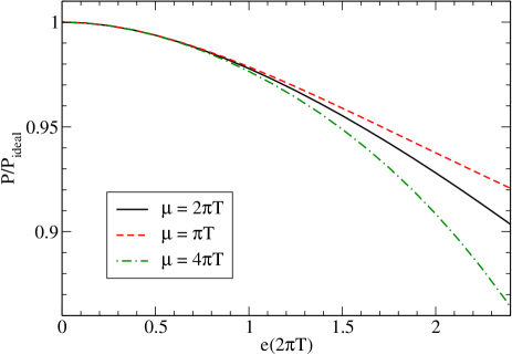
Figure 5: NLO HTLpt predictions for the free energy of QED with $N_{f}=1$ and the variational Debye mass. Different curves correspond to varying the renormalization scale $\mu$ by a factor of 2 around $\mu=2\pi T$.

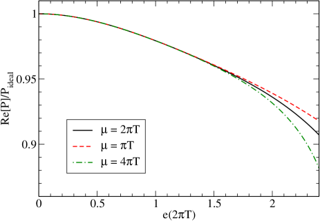
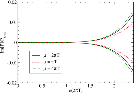
Figure 6: Real (top panel) and imaginary (bottom panel) parts of NNLO HTLpt predictions for the free energy of QED with $N_{f}=1$ and the variational Debye mass. Different curves correspond to varying the renormalization scale $\mu$ by a factor of 2 around $\mu=2\pi T$.

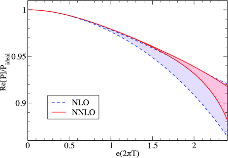
Figure 7: A comparison of the renormalization scale variations between NLO and NNLO HTLpt predictions for the free energy of QED with $N_{f}=1$ and the variational Debye mass. The bands correspond to varying the renormalization scale $\mu$ by a factor of 2 around $\mu=2\pi T$.

VI.2 Perturbative Debye and fermion masses

The perturbative Debye and fermion masses for QED have been calculated through order $e^{5}$ Blaizot:1995kg ; Andersen and $e^{3}$ carrington , respectively:

$$m_{D}^{2} = {1\over 3}N_{f}e^{2}T^{2}\Big{[}1-\frac{e^{2}}{24\pi^{2}}\left(4\gamma+7+4\log\frac{\hat{\mu}}{2}+8\log 2\right)$$ (75)

$$\hskip 42.67912pt+{e^{3}\sqrt{3}\over 4\pi^{3}}\Big{]}\;,$$

$$m_{f}^{2} = {1\over 8}N_{f}e^{2}T^{2}\left[1-{2.854\over 4\pi}e\right]\;.$$ (76)

Plugging (75) and (76) into the NLO and NNLO thermodynamic potentials, (69) and (72), we obtain the results shown in Fig. 8. The renormalization scale variation is quite small in the NNLO result.

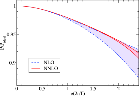
Figure 8: A comparison of the renormalization scale variations between NLO and NNLO HTLpt predictions for the free energy of QED with $N_{f}=1$ using the perturbative thermal masses given in Eqs. (75) and (76). The bands correspond to varying the renormalization scale $\mu$ by a factor of 2 around $\mu=2\pi T$.

VI.3 Comparison with the $\Phi$-derivable approach

Having obtained the NNLO HTLpt result for the free energy we can now compare the results obtained using this reorganization with results obtained within the $\Phi$-derivable approach. In Fig. 9 we show a comparison of our NNLO HTLpt results with a three-loop calculation obtained previously using a truncated three-loop $\Phi$-derivable approximation phijm . For the NNLO HTLpt prediction we show the results obtained using both the variational and perturbative mass prescriptions. As can be seen from this figure, there is very good agreement between the NNLO $\Phi$-derivable and HTLpt approaches out to large coupling. In all cases we have chosen the renormalization scale to be $\mu=2\pi T$.

As a further consistency check, in Fig. 10 we show a comparison between the untruncated two-loop numerical $\Phi$-derivable approach calculation of Ref. Borsanyi:2007bf and our NLO HTLpt result using the variational mass. In both cases we have chosen the renormalization scale to be $\mu=2\pi T$. From this figure we see that there is a reasonable agreement between the NLO numerical $\Phi$-derivable and NLO HTLpt results; however, the agreement is not as good as the corresponding NNLO results.

We note that the results of Borsanyi:2007bf were computed in the Landau gauge ($\xi=0$). As detailed in their paper, their result is gauge dependent. Such gauge dependence is unavoidable in the 2PI $\Phi$-derivable approach since it only uses dressed propagators. In Ref. phijm it was explicitly shown that the two-loop $\Phi$-derivable Debye mass is gauge independent only up to order $e^{2}$, resulting in gauge variation of the free energy at order $e^{4}$. This is in agreement with general theorems stating that the gauge variance appears at one order higher than the truncation Arrizabalaga:2002hn .

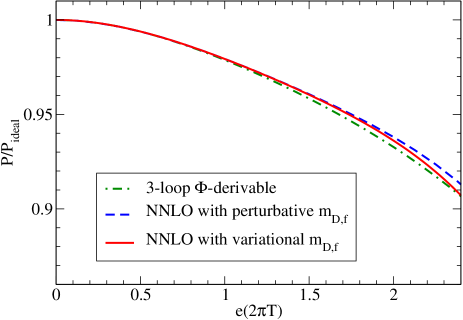
Figure 9: A comparison of the predictions for the free energy of QED with $N_{f}=1$ between three-loop $\Phi$-derivable approximation phijm and NNLO HTLpt at $\mu=2\pi T$.

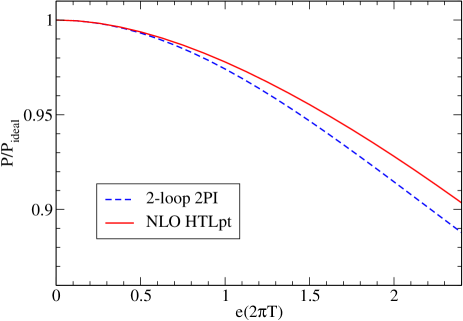
Figure 10: A comparison of the predictions for the free energy of QED with $N_{f}=1$ between the two-loop 2PI approximation in Landau gauge Borsanyi:2007bf and NLO HTLpt at $\mu=2\pi T$.

VII Conclusions

In this paper we calculated the three-loop HTLpt thermodynamic potential in QED. Having obtained this we applied two mass prescriptions, variational and perturbative, to fix the a priori undetermined parameters $m_{D}$ and $m_{f}$ that appear in the HTL-improved Lagrangian. We found that the resulting expressions for the free energy were the same to an accuracy of 0.6% at $e=2.4$ giving us confidence in the prediction. We also compared the HTLpt three-loop result with a three-loop $\Phi$-derivable approach phijm and found agreement at the subpercentage level at large coupling.

In addition, we showed that the HTLpt NLO and NNLO approximations have improved convergence at large coupling compared to the naively truncated weak-coupling expansion and that the renormalization scale variation at NNLO using both the variational and perturbative mass prescriptions was quite small. Therefore, the NNLO HTLpt method result seems to be quite reliable. This is important since, unlike the $\Phi$-derivable approach, the HTLpt reorganization is gauge invariant by construction and is formulated directly in Minkowski space allowing it to, in principle, also be applied to the calculation of dynamical quantities.

The renormalization of the three-loop thermodynamic potential required only known vacuum, mass, and coupling constant counterterms, and the resulting running coupling was found to coincide with the QED one-loop running. This provides further evidence that the HTLpt framework is renormalizable despite the new divergences which are introduced during HTL improvement.

Finally, we note that at three loops we could obtain an entirely analytic expression for the renormalized NNLO thermodynamic potential. There were a number of cancellations that took place during renormalization which resulted in an expression that was independent of any numerically determined subleading coefficients in the sum-integrals. We expect similar cancellations to also occur in non-Abelian gauge theories which will greatly simplify the calculation. Computing the three-loop HTLpt reorganized free energy for QCD is in progress.

Appendix A HTL Feynman Rules

In this appendix, we present Feynman rules for HTL perturbation theory in QED. We give explicit expressions for the propagators and for the electron-photon three- and four-vertices. The Feynman rules are given in Minkowski space to facilitate applications to real-time processes. A Minkowski momentum is denoted $p=(p_{0},{\bf p})$, and the inner product is $p\cdot q=p_{0}q_{0}-{\bf p}\cdot{\bf q}$. The vector that specifies the thermal rest frame is $n=(1,{\bf 0})$.

A.1 Photon self-energy

The HTL photon self-energy tensor for a photon of momentum $p$ is

$$\Pi^{\mu\nu}(p)=m_{D}^{2}\left[{\cal T}^{\mu\nu}(p,-p)-n^{\mu}n^{\nu}\right]\;.$$ (1)

The tensor ${\cal T}^{\mu\nu}(p,q)$, which is defined only for momenta that satisfy $p+q=0$, is

$${\cal T}^{\mu\nu}(p,-p)=\left\langle y^{\mu}y^{\nu}{p\!\cdot\!n\over p\!\cdot\!y}\right\rangle_{\bf\hat{y}}\;.$$ (2)

The angular brackets indicate averaging over the spatial directions of the lightlike vector $y=(1,\hat{\bf y})$. The tensor ${\cal T}^{\mu\nu}$ is symmetric in $\mu$ and $\nu$ and satisfies the “Ward identity”

$$p_{\mu}{\cal T}^{\mu\nu}(p,-p)=p\!\cdot\!n\;n^{\nu}\;.$$ (3)

The self-energy tensor $\Pi^{\mu\nu}$ is therefore also symmetric in $\mu$ and $\nu$ and satisfies

$$p_{\mu}\Pi^{\mu\nu}(p) = 0\;,$$ (4)

$$g_{\mu\nu}\Pi^{\mu\nu}(p) = -m_{D}^{2}\;.$$ (5)

The photon self-energy tensor can be expressed in terms of two scalar functions, the transverse and longitudinal self-energies $\Pi_{T}$ and $\Pi_{L}$, defined by

$$\Pi_{T}(p) = {1\over d-1}\left(\delta^{ij}-\hat{p}^{i}\hat{p}^{j}\right)\Pi^{ij}(p)\;,$$ (6)

$$\Pi_{L}(p) = -\Pi^{00}(p)\;,$$ (7)

where ${\bf\hat{p}}$ is the unit vector in the direction of ${\bf p}$. In terms of these functions, the self-energy tensor is

$$\Pi^{\mu\nu}(p)\;=\;-\Pi_{T}(p)T_{p}^{\mu\nu}-{1\over n_{p}^{2}}\Pi_{L}(p)L_{p}^{\mu\nu}\;,$$ (8)

where the tensors $T_{p}$ and $L_{p}$ are

$$T_{p}^{\mu\nu} = g^{\mu\nu}-{p^{\mu}p^{\nu}\over p^{2}}-{n_{p}^{\mu}n_{p}^{\nu}\over n_{p}^{2}}\;,$$ (9)

$$L_{p}^{\mu\nu} = {n_{p}^{\mu}n_{p}^{\nu}\over n_{p}^{2}}\;.$$ (10)

The four-vector $n_{p}^{\mu}$ is

$$n_{p}^{\mu}\;=\;n^{\mu}-{n\!\cdot\!p\over p^{2}}p^{\mu}$$ (11)

and satisfies $p\!\cdot\!n_{p}=0$ and $n^{2}_{p}=1-(n\!\cdot\!p)^{2}/p^{2}$. Equation (5) reduces to the identity

$$(d-1)\Pi_{T}(p)+{1\over n^{2}_{p}}\Pi_{L}(p)\;=\;m_{D}^{2}\;.$$ (12)

We can express both self-energy functions in terms of the function ${\cal T}^{00}$ defined by (2):

$$\Pi_{T}(p) = {m_{D}^{2}\over(d-1)n_{p}^{2}}\left[{\cal T}^{00}(p,-p)-1+n_{p}^{2}\right],$$ (13)

$$\Pi_{L}(p) = m_{D}^{2}\left[1-{\cal T}^{00}(p,-p)\right],$$ (14)

In the tensor ${\cal T}^{\mu\nu}(p,-p)$ defined in (2), the angular brackets indicate the angular average over the unit vector $\hat{\bf y}$. In almost all previous work, the angular average in (2) has been taken in $d=3$ dimensions. For consistency of higher-order radiative corrections, it is essential to take the angular average in $d=3-2\epsilon$ dimensions and analytically continue to $d=3$ only after all poles in $\epsilon$ have been cancelled. Expressing the angular average as an integral over the cosine of an angle, the expression for the $00$ component of the tensor is

$$\!\!\!{\cal T}^{00}(p,-p)\!\! = \!\!{w(\epsilon)\over 2}\!\!\int_{-1}^{1}\!\!dc\;(1-c^{2})^{-\epsilon}{p_{0}\over p_{0}-|{\bf p}|c}\,,$$ (15)

where the weight function $w(\epsilon)$ is

$$w(\epsilon)={\Gamma(2-2\epsilon)\over\Gamma^{2}(1-\epsilon)}2^{2\epsilon}={\Gamma({3\over 2}-\epsilon)\over\Gamma({3\over 2})\Gamma(1-\epsilon)}\;.$$ (16)

The integral in (15) must be defined so that it is analytic at $p_{0}=\infty$. It then has a branch cut running from $p_{0}=-|{\bf p}|$ to $p_{0}=+|{\bf p}|$. If we take the limit $\epsilon\rightarrow 0$, it reduces to

$${\cal T}^{00}(p,-p) = {p_{0}\over 2|{\bf p}|}\log{p_{0}+|{\bf p}|\over p_{0}-|{\bf p}|}\;,$$ (17)

which is the expression that appears in the usual HTL self-energy functions.

The Feynman rule for the photon propagator is

$$i\Delta_{\mu\nu}(p)\;,$$ (18)

where the photon propagator tensor $\Delta_{\mu\nu}$ depends on the choice of gauge fixing. We consider two possibilities that introduce an arbitrary gauge parameter $\xi$: general covariant gauge and general Coulomb gauge. In both cases, the inverse propagator reduces in the limit $\xi\rightarrow\infty$ to

$$\Delta^{-1}_{\infty}(p)^{\mu\nu} = -p^{2}g^{\mu\nu}+p^{\mu}p^{\nu}-\Pi^{\mu\nu}(p)\;.$$ (19)

This can also be written

$$\Delta^{-1}_{\infty}(p)^{\mu\nu} = -{1\over\Delta_{T}(p)}T_{p}^{\mu\nu}+{1\over n_{p}^{2}\Delta_{L}(p)}L_{p}^{\mu\nu}\;,$$ (20)

where $\Delta_{T}$ and $\Delta_{L}$ are the transverse and longitudinal propagators:

$$\Delta_{T}(p) = {1\over p^{2}-\Pi_{T}(p)}\;,$$ (21)

$$\Delta_{L}(p) = {1\over-n_{p}^{2}p^{2}+\Pi_{L}(p)}\;.$$ (22)

The inverse propagator for general $\xi$ is

$$\Delta^{-1}(p)^{\mu\nu} = \Delta^{-1}_{\infty}(p)^{\mu\nu}-{1\over\xi}p^{\mu}p^{\nu}\hskip 5.69046pt\mbox{covariant}\;,$$ (24)

$$= \Delta^{-1}_{\infty}(p)^{\mu\nu}-{1\over\xi}\left(p^{\mu}-p\!\cdot\!n\;n^{\mu}\right)\left(p^{\nu}-p\!\cdot\!n\;n^{\nu}\right)$$

$$\hskip 105.2751pt\mbox{Coulomb}\;.$$

The propagators obtained by inverting the tensors in (24) and (24) are

$$\Delta^{\mu\nu}(p) = -\Delta_{T}(p)T_{p}^{\mu\nu}+\Delta_{L}(p)n_{p}^{\mu}n_{p}^{\nu}-\xi{p^{\mu}p^{\nu}\over(p^{2})^{2}}$$ (26)

$$\hskip 105.2751pt\mbox{covariant}\;,$$

$$= -\Delta_{T}(p)T_{p}^{\mu\nu}+\Delta_{L}(p)n^{\mu}n^{\nu}-\xi{p^{\mu}p^{\nu}\over\left(n_{p}^{2}p^{2}\right)^{2}}$$

$$\hskip 105.2751pt\mbox{Coulomb}\;.$$

It is convenient to define the following combination of propagators:

$$\Delta_{X}(p) = \Delta_{L}(p)+{1\over n_{p}^{2}}\Delta_{T}(p)\;.$$ (27)

Using (12), (21), and (22), it can be expressed in the alternative form

$$\Delta_{X}(p) = \left[m_{D}^{2}-d\,\Pi_{T}(p)\right]\Delta_{L}(p)\Delta_{T}(p)\;,$$ (28)

which shows that it vanishes in the limit $m_{D}\to 0$. In the covariant gauge, the propagator tensor can be written

$$\Delta^{\mu\nu}(p) = \left[-\Delta_{T}(p)g^{\mu\nu}+\Delta_{X}(p)n^{\mu}n^{\nu}\right]$$

$$-{n\!\cdot\!p\over p^{2}}\Delta_{X}(p)\left(p^{\mu}n^{\nu}+n^{\mu}p^{\nu}\right)$$

$$+\left[\Delta_{T}(p)+{(n\!\cdot\!p)^{2}\over p^{2}}\Delta_{X}(p)-{\xi\over p^{2}}\right]{p^{\mu}p^{\nu}\over p^{2}}\;.$$

This decomposition of the propagator into three terms has proved to be particularly convenient for explicit calculations. For example, the first term satisfies the identity

$$\left[-\Delta_{T}(p)g_{\mu\nu}+\Delta_{X}(p)n_{\mu}n_{\nu}\right]\Delta^{-1}_{\infty}(p)^{\nu\lambda} =$$ (30)

$${g_{\mu}}^{\lambda}-{p_{\mu}p^{\lambda}\over p^{2}}+{n\!\cdot\!p\over n_{p}^{2}p^{2}}{\Delta_{X}(p)\over\Delta_{L}(p)}p_{\mu}n_{p}^{\lambda}\;.$$

A.2 Electron self-energy

The HTL self-energy of an electron with momentum $p$ is given by

$$\Sigma(P)=m_{f}^{2}/\!\!\!\!{\cal T}(p)\;,$$ (31)

where

$${\cal T}^{\mu}(p)=\left\langle{y^{\mu}\over p\cdot y}\right\rangle_{\hat{\bf y}}\;.$$ (32)

Expressing the angular average as an integral over the cosine of an angle, the expression is

$${\cal T}^{\mu}(p)={w(\epsilon)\over 2}\int_{-1}^{1}dc\;(1-c^{2})^{-\epsilon}{y^{\mu}\over p_{0}-|{\bf p}|c}\;,$$ (33)

The integral in (33) must be defined so that it is analytic at $p_{0}=\infty$. It then has a branch cut running from $p_{0}=-|{\bf p}|$ to $p_{0}=+|{\bf p}|$. In three dimensions, this reduces to

$$\Sigma(P) = {m_{f}^{2}\over 2|{\bf p}|}\gamma_{0}\log{p_{0}+|{\bf p}|\over p_{0}-|{\bf p|}}$$ (34)

$$\!\!\!+{m_{f}^{2}\over|{\bf p}|}{\bf\gamma}\cdot\hat{\bf p}\left(1-{p_{0}\over 2|{\bf p}|}\log{p_{0}+|{\bf p}|\over p_{0}-|{\bf p|}}\right).$$

A.3 Electron propagator

The Feynman rule for the electron propagator is

$$iS(p)\;.$$ (35)

The electron propagator can be written as

$$S(p)={1\over/\!\!\!p-\Sigma(p)}\;,$$ (36)

where the electron self-energy is given by (31). The inverse electron propagator can be written as

$$S^{-1}(p)=/\!\!\!p-\Sigma(p)\;.$$ (37)

This can be written as

$$S^{-1}(p)=/\!\!\!\!{\cal A}(p)\;,$$ (38)

where we have organized $A_{0}(p)$ and $A_{S}(p)$ into:

$$A_{\mu}(p)=(A_{0}(p),A_{S}(p)\hat{\bf p})\;.$$ (39)

The functions $A_{0}(p)$ and $A_{S}(p)$ are defined

$$A_{0}(p) = p_{0}-{m_{f}^{2}\over p_{0}}{\cal T}_{p}\;,$$ (40)

$$A_{S}(p) = |{\bf p}|+{m_{f}^{2}\over|{\bf p}|}\left[1-{\cal T}_{p}\right]\;.$$ (41)

A.4 Electron-photon vertex

The electron-photon vertex with outgoing photon momentum $p$, incoming electron momentum $q$, outgoing electron momentum $r$, and Lorentz index $\mu$ is

$$\Gamma^{\mu}(p,q,r)=e\left(\gamma^{\mu}-m_{f}^{2}\tilde{{\cal T}}^{\mu}(p,q,r)\right)\;.$$ (42)

The tensor in the HTL correction term is only defined for $p-q+r=0$:

$$\tilde{{\cal T}}^{\mu}(p,q,r)=\left\langle y^{\mu}\left({y\!\!\!/\over q\!\cdot\!y\;\;r\!\cdot\!y}\right)\right\rangle_{\hat{\bf y}}.$$ (43)

This tensor is even under the permutation of $q$ and $r$. It satisfies the “Ward identity”

$$\!\!\!p_{\mu}\tilde{\cal T}^{\mu}(p,q,r)=\tilde{\cal T}^{\mu}(q)-\tilde{\cal T}^{\mu}(r)\;,$$ (44)

The electron-photon vertex therefore satisfies the Ward identity

$$p_{\mu}\Gamma^{\mu}(p,q,r)=S^{-1}(q)-S^{-1}(r)\;.$$ (45)

A.5 Electron-photon four-vertex

We define the electron-photon four-point vertex with outgoing photon momenta $p$ and $q$, incoming electron momentum $r$, and outgoing electron momentum $s$. It reads

$$\Gamma^{\mu\nu}(p,q,r,s) = -2e^{2}m_{f}^{2}\tilde{\cal T}^{\mu\nu}(p,q,r,s)$$ (46)

$$\equiv 2e^{2}\Gamma^{\mu\nu}\,,$$

There is no tree-level term. The tensor in the HTL correction term is only defined for $p+q-r+s=0$,

$$\tilde{{\cal T}}^{\mu\nu}(p,q,r,s) = \left\langle y^{\mu}y^{\nu}\left({1\over r\!\cdot\!y}+{1\over s\!\cdot\!y}\right)\right.$$ (47)

$$\times\left.{y\!\!\!/\over[(r-p)\!\cdot\!y]\;[(s+p)\!\cdot\!y]}\right\rangle.$$

This tensor is symmetric in $\mu$ and $\nu$ and is traceless. It satisfies the Ward identity:

$$\!\!p_{\mu}\Gamma^{\mu\nu}(p,q,r,s)\!=\!\Gamma^{\nu}(q,r-p,s)-\Gamma^{\nu}(q,r,s+p)\,.$$ (48)

A.6 HTL electron counterterm

The Feynman rule for the insertion of an HTL electron counterterm into an electron propagator is

$$i\Sigma(p)\;,$$ (49)

where $\Sigma(p)$ is the HTL electron self-energy given in (39).

A.7 Imaginary-time formalism

In the imaginary-time formalism, Minkowski energies have discrete imaginary values $p_{0}=i(2\pi nT)$ and integrals over Minkowski space are replaced by sum-integrals over Euclidean vectors $(2\pi nT,{\bf p})$. We will use the notation $P=(P_{0},{\bf p})$ for Euclidean momenta. The magnitude of the spatial momentum will be denoted $p=|{\bf p}|$, and should not be confused with a Minkowski vector. The inner product of two Euclidean vectors is $P\cdot Q=P_{0}Q_{0}+{\bf p}\cdot{\bf q}$. The vector that specifies the thermal rest frame remains $n=(1,{\bf 0})$.

The Feynman rules for Minkowski space given above can be easily adapted to Euclidean space. The Euclidean tensor in a given Feynman rule is obtained from the corresponding Minkowski tensor with raised indices by replacing each Minkowski energy $p_{0}$ by $iP_{0}$, where $P_{0}$ is the corresponding Euclidean energy, and multipying by $-i$ for every $0$ index. This prescription transforms $p=(p_{0},{\bf p})$ into $P=(P_{0},{\bf p})$, $g^{\mu\nu}$ into $-\delta^{\mu\nu}$, and $p\!\cdot\!q$ into $-P\!\cdot\!Q$. The effect on the HTL tensors defined in (2), (43), and (47) is equivalent to substituting $p\!\cdot\!n\to-P\!\cdot\!N$ where $N=(-i,{\bf 0})$, $p\!\cdot\!y\to-P\!\cdot\!Y$ where $Y=(-i,{\bf\hat{y}})$, and $y^{\mu}\to Y^{\mu}$. For example, the Euclidean tensor corresponding to (2) is

$${\cal T}^{\mu\nu}(P,-P)=\left\langle Y^{\mu}Y^{\nu}{P\!\cdot\!N\over P\!\cdot\!Y}\right\rangle\;.$$ (50)

The average is taken over the directions of the unit vector ${\bf\hat{y}}$.

Alternatively, one can calculate a diagram by using the Feynman rules for Minkowski momenta, reducing the expressions for diagrams to scalars, and then make the appropriate substitutions, such as $p^{2}\to-P^{2}$, $p\cdot q\to-P\cdot Q$, and $n\cdot p\to in\cdot P$. For example, the propagator functions (21) and (22) become

$$\Delta_{T}(P) = {-1\over P^{2}+\Pi_{T}(P)}\;,$$ (51)

$$\Delta_{L}(P) = {1\over p^{2}+\Pi_{L}(P)}\;.$$ (52)

The expressions for the HTL self-energy functions $\Pi_{T}(P)$ and $\Pi_{L}(P)$ are given by (13) and (14) with $n_{p}^{2}$ replaced by $n_{P}^{2}=p^{2}/P^{2}$ and ${\cal T}^{00}(p,-p)$ replaced by

$${\cal T}_{P} = {w(\epsilon)\over 2}\int_{-1}^{1}dc\;(1-c^{2})^{-\epsilon}{iP_{0}\over iP_{0}-pc}\;.$$ (53)

Note that this function differs by a sign from the 00 component of the Euclidean tensor corresponding to (2):

$${\cal T}^{00}(P,-P)=-{\cal T}^{00}(p,-p)\bigg{|}_{p_{0}\to iP_{0}}=-{\cal T}_{P}\;.$$ (54)

A more convenient form for calculating sum-integrals that involve the function ${\cal T}_{P}$ is

$${\cal T}_{P} = \left\langle{P_{0}^{2}\over P_{0}^{2}+p^{2}c^{2}}\right\rangle_{\!\!c}\,,$$ (55)

where the angular brackets represent an average over $c$ defined by

$$\left\langle f(c)\right\rangle_{\!c}\equiv w(\epsilon)\int_{0}^{1}dc\,(1-c^{2})^{-\epsilon}f(c)\,,$$ (56)

and $w(\epsilon)$ is given in (16).

Appendix B Sum-integrals

In the imaginary-time formalism for thermal field theory, the four-momentum $P=(P_{0},{\bf p})$ is Euclidean with $P^{2}=P_{0}^{2}+{\bf p}^{2}$. The Euclidean energy $p_{0}$ has discrete values: $P_{0}=2n\pi T$ for bosons and $P_{0}=(2n+1)\pi T$ for fermions, where $n$ is an integer. Loop diagrams involve sums over $P_{0}$ and integrals over ${\bf p}$. With dimensional regularization, the integral is generalized to $d=3-2\epsilon$ spatial dimensions. We define the dimensionally regularized sum-integral by

$$\hbox{$\sum$}\!\!\!\!\!\!\int_{P} \equiv \left(\frac{e^{\gamma}\mu^{2}}{4\pi}\right)^{\epsilon}\;T\sum_{P_{0}=2n\pi T}\>\int{d^{3-2\epsilon}p\over(2\pi)^{3-2\epsilon}}\;,$$ (1)

$$\hbox{$\sum$}\!\!\!\!\!\!\int_{\{P\}}\!\!\! \equiv \!\!\!\left(\frac{e^{\gamma}\mu^{2}}{4\pi}\right)^{\epsilon}\;T\sum_{P_{0}=(2n+1)\pi T}\>\int{d^{3-2\epsilon}p\over(2\pi)^{3-2\epsilon}}\;,$$ (2)

where $3-2\epsilon$ is the dimension of space and $\mu$ is an arbitrary momentum scale. The factor $(e^{\gamma}/4\pi)^{\epsilon}$ is introduced so that, after minimal subtraction of the poles in $\epsilon$ due to ultraviolet divergences, $\mu$ coincides with the renormalization scale of the $\overline{\rm MS}$ renormalization scheme.

Below we list the sum-integrals required to complete the three-loop calculation. We refer to htl2 ; aps1 for details concerning the sum-integral evaluations.

B.1 One-loop sum-integrals

The simple one-loop sum-integrals required in our calculations can be derived from the formulas

$$\hbox{$\sum$}\!\!\!\!\!\!\!\int_{P}{p^{2m}\over(P^{2})^{n}}\!\! = \!\!\left({\mu\over 4\pi T}\right)^{2\epsilon}{2\Gamma({3\over 2}+m-\epsilon)\Gamma(n-{3\over 2}-m+\epsilon)\over\Gamma(n)\Gamma(2-2\epsilon)}$$ (3)

$$\;\times\,\Gamma(1-\epsilon)\zeta(2n-2m-3+2\epsilon)e^{\epsilon\gamma}$$

$$\;\;\;\;\times\,T^{4+2m-2n}(2\pi)^{1+2m-2n}\;,$$

$$\hbox{$\sum$}\!\!\!\!\!\!\!\int_{\{P\}}\!\!{p^{2m}\over(P^{2})^{n}}\!\! = \!\!(2^{2n-2m-d}-1)\hbox{$\sum$}\!\!\!\!\!\!\!\int_{P}{p^{2m}\over(P^{2})^{n}}\;.$$ (4)

The specific bosonic one-loop sum-integrals needed are

$$\hbox{$\sum$}\!\!\!\!\!\!\!\int_{P}\log P^{2} = -{\pi^{2}\over 45}T^{4}\left[1+{\cal O}\!\left(\epsilon\right)\right]\;,$$ (5)

$$\hbox{$\sum$}\!\!\!\!\!\!\!\int_{P}{1\over P^{2}} = {T^{2}\over 12}\left({\mu\over 4\pi T}\right)^{2\epsilon}\Bigg{[}1+\left(2+2{\zeta^{\prime}(-1)\over\zeta(-1)}\right)\epsilon+{\cal O}\!\left(\epsilon^{2}\right)\Bigg{]}\;,$$ (6)

$$\hbox{$\sum$}\!\!\!\!\!\!\!\int_{P}{1\over(P^{2})^{2}} = {1\over(4\pi)^{2}}\left({\mu\over 4\pi T}\right)^{2\epsilon}\left[{1\over\epsilon}+2\gamma+{\cal O}\!\left(\epsilon\right)\right]\;,$$ (7)

$$\hbox{$\sum$}\!\!\!\!\!\!\!\int_{P}{1\over p^{2}P^{2}} = {1\over(4\pi)^{2}}\left({\mu\over 4\pi T}\right)^{2\epsilon}2\left[{1\over\epsilon}+2\gamma+2+{\cal O}\!\left(\epsilon\right)\right]\;.$$ (8)

The specific fermionic one-loop sum-integrals needed are

$$\hbox{$\sum$}\!\!\!\!\!\!\!\int_{\{P\}}\log P^{2} = {7\pi^{2}\over 360}T^{4}\left[1+{\cal O}\!\left(\epsilon\right)\right]\;,$$ (9)

$$\hbox{$\sum$}\!\!\!\!\!\!\!\int_{\{P\}}{1\over P^{2}} = -{T^{2}\over 24}\left({\mu\over 4\pi T}\right)^{2\epsilon}\bigg{[}1+\bigg{(}2-2\log 2+2{\zeta^{\prime}(-1)\over\zeta(-1)}\bigg{)}\epsilon+{\cal O}\!\left(\epsilon^{2}\right)\bigg{]}\;,$$ (10)

$$\hbox{$\sum$}\!\!\!\!\!\!\!\int_{\{P\}}{1\over(P^{2})^{2}} = {1\over(4\pi)^{2}}\left({\mu\over 4\pi T}\right)^{2\epsilon}\left[{1\over\epsilon}+2\gamma+4\log 2+{\cal O}\!\left(\epsilon\right)\right],$$ (11)

$$\hbox{$\sum$}\!\!\!\!\!\!\!\int_{\{P\}}{p^{2}\over(P^{2})^{2}} = -{T^{2}\over 16}\left({\mu\over 4\pi T}\right)^{2\epsilon}\bigg{[}1+\bigg{(}{4\over 3}-2\log 2+2{\zeta^{\prime}(-1)\over\zeta(-1)}\bigg{)}\epsilon+{\cal O}\!\left(\epsilon^{2}\right)\bigg{]}\;,$$ (12)

$$\hbox{$\sum$}\!\!\!\!\!\!\!\int_{\{P\}}{p^{2}\over(P^{2})^{3}} = {1\over(4\pi)^{2}}\left({\mu\over 4\pi T}\right)^{2\epsilon}\,{3\over 4}\bigg{[}{1\over\epsilon}+2\gamma-{2\over 3}+4\log 2+{\cal O}\!\left(\epsilon\right)\bigg{]},$$ (13)

$$\hbox{$\sum$}\!\!\!\!\!\!\!\int_{\{P\}}{p^{4}\over(P^{2})^{4}} = {1\over(4\pi)^{2}}\left({\mu\over 4\pi T}\right)^{2\epsilon}{5\over 8}\bigg{[}{1\over\epsilon}+2\gamma-{16\over 15}+4\log 2+{\cal O}\!\left(\epsilon\right)\bigg{]}\;,$$ (14)

$$\hbox{$\sum$}\!\!\!\!\!\!\!\int_{\{P\}}{1\over p^{2}P^{2}} = {1\over(4\pi)^{2}}\left({\mu\over 4\pi T}\right)^{2\epsilon}2\bigg{[}{1\over\epsilon}+2+2\gamma+4\log 2+{\cal O}\!\left(\epsilon\right)\bigg{]}\;.$$ (15)

The errors are all of one order higher in $\epsilon$ than the smallest term shown. The number $\gamma_{1}$ is the first Stieltjes gamma constant defined by the equation

$$\zeta(1+z)={1\over z}+\gamma-\gamma_{1}z+O(z^{2})\;.$$ (16)

We also need some more difficult one-loop sum-integrals that involve the HTL function defined in (33). The specific bosonic sum-integrals needed are

$$\hbox{$\sum$}\!\!\!\!\!\!\!\int_{P}{1\over p^{4}}{\cal T}_{P} = {1\over(4\pi)^{2}}\left({\mu\over 4\pi T}\right)^{2\epsilon}(-1)\left[{1\over\epsilon}+2\gamma+2\log 2+{\cal O}\!\left(\epsilon\right)\right]\;,$$ (17)

$$\hbox{$\sum$}\!\!\!\!\!\!\!\int_{P}{1\over p^{2}P^{2}}{\cal T}_{P} = {1\over(4\pi)^{2}}\left({\mu\over 4\pi T}\right)^{2\epsilon}\left[2\log 2\left({1\over\epsilon}+2\gamma\right)+2\log^{2}2+{\pi^{2}\over 3}+{\cal O}\!\left(\epsilon\right)\right]\;,$$ (18)

$$\hbox{$\sum$}\!\!\!\!\!\!\!\int_{P}{1\over p^{4}}({\cal T}_{P})^{2} = {1\over(4\pi)^{2}}\left({\mu\over 4\pi T}\right)^{2\epsilon}\left(-{2\over 3}\right)\left[(1+2\log 2)\left({1\over\epsilon}+2\gamma\right)-{4\over 3}+{22\over 3}\log 2+2\log^{2}2+{\cal O}\!\left(\epsilon\right)\right]\;.$$ (19)

The specific fermionic sum-integrals needed are

$$\hbox{$\sum$}\!\!\!\!\!\!\!\int_{\{P\}}{1\over(P^{2})^{2}}{\cal T}_{P} = {1\over(4\pi)^{2}}\left({\mu\over 4\pi T}\right)^{2\epsilon}{1\over 2}\bigg{[}{1\over\epsilon}+2\gamma+1+4\log 2+{\cal O}\!\left(\epsilon\right)\bigg{]}\;,$$ (20)

$$\hbox{$\sum$}\!\!\!\!\!\!\!\int_{\{P\}}{1\over p^{2}P^{2}}{\cal T}_{P} = {1\over(4\pi)^{2}}\left({\mu\over 4\pi T}\right)^{2\epsilon}\left[2\log 2\left({1\over\epsilon}+2\gamma\right)+10\log^{2}2+{\pi^{2}\over 3}+{\cal O}\!\left(\epsilon\right)\right]\;,$$ (21)

$$\hbox{$\sum$}\!\!\!\!\!\!\!\int_{\{P\}}{1\over P^{2}P_{0}^{2}}{\cal T}_{P} = {1\over(4\pi)^{2}}\left({\mu\over 4\pi T}\right)^{2\epsilon}\Bigg{[}{1\over\epsilon^{2}}+2(\gamma+2\log 2){1\over\epsilon}+{\pi^{2}\over 4}+4\log^{2}2+8\gamma\log 2-4\gamma_{1}+{\cal O}\!\left(\epsilon\right)\bigg{]}\;,$$ (22)

$$\hbox{$\sum$}\!\!\!\!\!\!\!\int_{\{P\}}{1\over p^{2}P_{0}^{2}}\left({\cal T}_{P}\right)^{2} = {4\over(4\pi)^{2}}\left({\mu\over 4\pi T}\right)^{2\epsilon}\bigg{[}\log 2\left({1\over\epsilon}+2\gamma\right)+5\log^{2}2+{\cal O}\!\left(\epsilon\right)\bigg{]}\;,$$ (23)

$$\hbox{$\sum$}\!\!\!\!\!\!\!\int_{\{P\}}{1\over P^{2}}\bigg{\langle}{1\over(P\!\cdot\!Y)^{2}}\bigg{\rangle}_{\hat{\bf y}} = {1\over(4\pi)^{2}}\left({\mu\over 4\pi T}\right)^{2\epsilon}(-1)\bigg{[}{1\over\epsilon}-1+2\gamma+4\log 2+{\cal O}\!\left(\epsilon\right)\bigg{]}\;.$$ (24)

B.2 Two-loop sum-integrals

The simple two-loop sum-integrals that are needed are

$$\hbox{$\sum$}\!\!\!\!\!\!\!\int_{\{PQ\}}{1\over P^{2}Q^{2}R^{2}} = 0\;,$$ (25)

$$\hbox{$\sum$}\!\!\!\!\!\!\!\int_{\{PQ\}}{1\over P^{2}Q^{2}r^{2}} = {T^{2}\over(4\pi)^{2}}\left({\mu\over 4\pi T}\right)^{4\epsilon}\left(-{1\over 6}\right)\left[{1\over\epsilon}+4-2\log 2+4{\zeta^{\prime}(-1)\over\zeta(-1)}+{\cal O}\!\left(\epsilon\right)\right]\;,$$ (26)

$$\hbox{$\sum$}\!\!\!\!\!\!\!\int_{\{PQ\}}{q^{2}\over P^{2}Q^{2}r^{4}} = {T^{2}\over(4\pi)^{2}}\left({\mu\over 4\pi T}\right)^{4\epsilon}\left(-{1\over 12}\right)\left[{1\over\epsilon}+{11\over 3}+2\gamma-2\log 2+2{\zeta^{\prime}(-1)\over\zeta(-1)}+{\cal O}\!\left(\epsilon\right)\right],$$ (27)

$$\hbox{$\sum$}\!\!\!\!\!\!\!\int_{\{PQ\}}{q^{2}\over P^{2}Q^{2}r^{2}R^{2}} = {T^{2}\over(4\pi)^{2}}\left({\mu\over 4\pi T}\right)^{4\epsilon}\left(-{1\over 72}\right)\bigg{[}{1\over\epsilon}-7.00164+{\cal O}\!\left(\epsilon\right)\bigg{]}\;,$$ (28)

$$\hbox{$\sum$}\!\!\!\!\!\!\!\int_{\{PQ\}}{P\!\cdot\!Q\over P^{2}Q^{2}r^{4}} = {T^{2}\over(4\pi)^{2}}\left({\mu\over 4\pi T}\right)^{4\epsilon}\left(-{1\over 36}\right)\left[1-6\gamma+6{\zeta^{\prime}(-1)\over\zeta(-1)}+{\cal O}\!\left(\epsilon\right)\right]\;,$$ (29)

$$\hbox{$\sum$}\!\!\!\!\!\!\!\int_{\{PQ\}}{p^{2}\over q^{2}P^{2}Q^{2}R^{2}} = {T^{2}\over(4\pi)^{2}}\left({\mu\over 4\pi T}\right)^{4\epsilon}\left({5\over 72}\right)\left[{1\over\epsilon}+9.55216+{\cal O}\!\left(\epsilon\right)\right]\;,$$ (30)

$$\hbox{$\sum$}\!\!\!\!\!\!\!\int_{\{PQ\}}{r^{2}\over q^{2}P^{2}Q^{2}R^{2}} = {T^{2}\over(4\pi)^{2}}\left({\mu\over 4\pi T}\right)^{4\epsilon}\left(-{1\over 18}\right)\left[{1\over\epsilon}+8.14234+{\cal O}\!\left(\epsilon\right)\right],$$ (31)

where $R=-(P+Q)$ and $r=|{\bf p}+{\bf q}|$. The corrections are all of order $\epsilon^{2}$. We also need some more difficult two-loop sum-integrals that involve the functions ${\cal T}_{P}$ defined in (33),

$$\hbox{$\sum$}\!\!\!\!\!\!\!\int_{\{PQ\}}{1\over P^{2}Q^{2}r^{2}}{\cal T}_{R} = {T^{2}\over(4\pi)^{2}}\left({\mu\over 4\pi T}\right)^{4\epsilon}\left(-{1\over 48}\right)\Bigg{[}{1\over\epsilon^{2}}+\left(2+12\log 2+4{\zeta^{\prime}(-1)\over\zeta(-1)}\right){1\over\epsilon}+136.362\,\,+{\cal O}\!\left(\epsilon\right)\Bigg{]}\,,$$ (32)

$$\hbox{$\sum$}\!\!\!\!\!\!\!\int_{\{PQ\}}{q^{2}\over P^{2}Q^{2}r^{4}}{\cal T}_{R} = {T^{2}\over(4\pi)^{2}}\left({\mu\over 4\pi T}\right)^{4\epsilon}\left(-{1\over 576}\right)\Bigg{[}{1\over\epsilon^{2}}+\left({26\over 3}+52\log 2+4{\zeta^{\prime}(-1)\over\zeta(-1)}\right){1\over\epsilon}+446.412+{\cal O}\!\left(\epsilon\right)\!\Bigg{]}\!,$$ (33)

$$\hbox{$\sum$}\!\!\!\!\!\!\!\int_{\{PQ\}}{P\!\cdot\!Q\over P^{2}Q^{2}r^{4}}{\cal T}_{R} = {T^{2}\over(4\pi)^{2}}\left({\mu\over 4\pi T}\right)^{4\epsilon}\left(-{1\over 96}\right)\Bigg{[}{1\over\epsilon^{2}}+\left(4\log 2+4{\zeta^{\prime}(-1)\over\zeta(-1)}\right){1\over\epsilon}+69.174+{\cal O}\!\left(\epsilon\right)\Bigg{]}\;,$$ (34)

$$\hbox{$\sum$}\!\!\!\!\!\!\!\int_{\{PQ\}}{r^{2}-p^{2}\over P^{2}q^{2}Q^{2}_{0}R^{2}}{\cal T}_{Q} = -{T^{2}\over(4\pi)^{2}}\left({\mu\over 4\pi T}\right)^{4\epsilon}{1\over 8}\Bigg{[}{1\over\epsilon^{2}}+\left(2+2\gamma+{10\over 3}\log 2+2{\zeta^{\prime}(-1)\over\zeta(-1)}\right){1\over\epsilon}+46.8757+{\cal O}\!\left(\epsilon\right)\Bigg{]}\;.$$ (35)

B.3 Three-loop sum-integrals

The three-loop sum-integrals needed are

$$\hbox{$\sum$}\!\!\!\!\!\!\!\int_{PQR}{1\over P^{2}Q^{2}R^{2}(P+Q+R)^{2}} = {1\over(4\pi)^{2}}\left({T^{2}\over 12}\right)^{2}\left({\mu\over 4\pi T}\right)^{6\epsilon}\left[{6\over\epsilon}+{182\over 5}-12{\zeta^{\prime}(-3)\over\zeta(-3)}+48{\zeta^{\prime}(-1)\over\zeta(-1)}+{\cal O}\!\left(\epsilon\right)\right],$$ (36)

$$\hbox{$\sum$}\!\!\!\!\!\!\!\int_{\{PQR\}}{1\over P^{2}Q^{2}R^{2}(P+Q+R)^{2}} = {1\over(4\pi)^{2}}\left({T^{2}\over 12}\right)^{2}\left({\mu\over 4\pi T}\right)^{6\epsilon}\left[{3\over 2\epsilon}+{173\over 20}-{63\over 5}\log 2-3{\zeta^{\prime}(-3)\over\zeta(-3)}\right.$$ (37)

$$\left.+12{\zeta^{\prime}(-1)\over\zeta(-1)}+{\cal O}\!\left(\epsilon\right)\right]\;,$$

$$\hbox{$\sum$}\!\!\!\!\!\!\!\int_{PQ\{R\}}{1\over P^{2}Q^{2}R^{2}(P+Q+R)^{2}} = {1\over(4\pi)^{2}}\left({T^{2}\over 12}\right)^{2}\left({\mu\over 4\pi T}\right)^{6\epsilon}\left[-{3\over 4\epsilon}-{179\over 40}+{51\over 10}\log 2+{3\over 2}{\zeta^{\prime}(-3)\over\zeta(-3)}-6{\zeta^{\prime}(-1)\over\zeta(-1)}\right.$$ (38)

$$+{\cal O}\!\left(\epsilon\right)\biggr{]}\;,$$

$$\hbox{$\sum$}\!\!\!\!\!\!\!\int_{\{P\}QR}{Q\!\cdot\!R\over P^{2}Q^{2}R^{2}(P+Q)^{2}(P+R)^{2}} = {1\over(4\pi)^{2}}\left({T^{2}\over 12}\right)^{2}\left({\mu\over 4\pi T}\right)^{6\epsilon}\left[{3\over 8\epsilon}+{9\over 4}\gamma+{361\over 160}+{57\over 10}\log 2+{3\over 2}{\zeta^{\prime}(-3)\over\zeta(-3)}\right.$$ (39)

$$\left.-{3\over 2}{\zeta^{\prime}(-1)\over\zeta(-1)}+{\cal O}\!\left(\epsilon\right)\right]\;,$$

$$\hbox{$\sum$}\!\!\!\!\!\!\!\int_{P\{QR\}}{(Q\!\cdot\!R)^{2}\over P^{2}Q^{2}R^{2}(P+Q)^{2}(P+R)^{2}} = {1\over(4\pi)^{2}}\left({T^{2}\over 12}\right)^{2}\left({\mu\over 4\pi T}\right)^{6\epsilon}\left[{5\over 24\epsilon}+{1\over 4}\gamma+{23\over 24}-{8\over 5}\log 2-{1\over 6}{\zeta^{\prime}(-3)\over\zeta(-3)}\right.$$ (40)

$$\left.+{7\over 6}{\zeta^{\prime}(-1)\over\zeta(-1)}+{\cal O}\!\left(\epsilon\right)\right]\;.$$

The three-loop sum-integrals were first calculated by Arnold and Zhai, and calculational details can be found in Ref. AZ-95 .

Appendix C Three-dimensional integrals

Dimensional regularization can be used to regularize both the ultraviolet divergences and infrared divergences in three-dimensional integrals over momenta. The spatial dimension is generalized to $d=3-2\epsilon$ dimensions. Integrals are evaluated at a value of $d$, for which they converge, and then analytically continued to $d=3$. We use the integration measure

$$\int_{p}\;\equiv\;\left(\frac{e^{\gamma}\mu^{2}}{4\pi}\right)^{\epsilon}\;\>\int{d^{3-2\epsilon}p\over(2\pi)^{3-2\epsilon}}\;.$$ (41)

The one-loop integrals needed are of the form

$$I_{n} \equiv \int_{p}{1\over(p^{2}+m^{2})^{n}}$$ (42)

$$= {1\over 8\pi}(e^{\gamma_{E}}\mu^{2})^{\epsilon}{\Gamma(n-\mbox{$3\over 2$}+\epsilon)\over\Gamma(\mbox{$1\over 2$})\Gamma(n)}m^{3-2n-2\epsilon}\;.$$

Specifically, we need

$$I_{0}^{\prime} \equiv \int_{p}\log(p^{2}+m^{2})$$ (43)

$$= -{m^{3}\over 6\pi}\left({\mu\over 2m}\right)^{2\epsilon}\left[1+{8\over 3}\epsilon+{\cal O}\!\left(\epsilon^{2}\right)\right]\;,$$

$$I_{1} = -{m\over 4\pi}\left({\mu\over 2m}\right)^{2\epsilon}\left[1+2\epsilon+{\cal O}\!\left(\epsilon^{2}\right)\right]\;,$$ (44)

$$I_{2} = {1\over 8\pi m}\left({\mu\over 2m}\right)^{2\epsilon}\left[1+{\cal O}\!\left(\epsilon\right)\right]\;.$$ (45)

References

• (1) J. Frenkel, A.V. Saa and J.C. Taylor, Phys. Rev. D46, 3670 (1992).
• (2) P. Arnold and C. X. Zhai, Phys. Rev. D 50, 7603 (1994); Phys. Rev. D 51, 1906 (1995).
• (3) R.R. Parwani and C. Corianò, Nucl. Phys. B434, 56 (1995).
• (4) R.R. Parwani and H. Singh, Phys. Rev. D51, 4518 (1995).
• (5) E. Braaten and A. Nieto, Phys. Rev. D51, 6990 (1995).
• (6) R.R. Parwani, Phys. Lett. B334, 420 (1994);
• (7) J.O. Andersen, Phys. Rev. D53, 7286 (1996).
• (8) C. X. Zhai and B. Kastening, Phys. Rev. D52, 7232 (1995).
• (9) E. Braaten and A. Nieto, Phys. Rev. Lett.  76, 1417 (1996); Phys. Rev. D53, 3421 (1996).
• (10) K. Kajantie, M. Laine, K. Rummukainen and Y. Schroder, Phys. Rev.  D 67, 105008 (2003) [arXiv:hep-ph/0211321].
• (11) A. Gynther, M. Laine, Y. Schroder, C. Torrero and A. Vuorinen, JHEP 0704, 094 (2007) [arXiv:hep-ph/0703307].
• (12) J. O. Andersen, L. Kyllingstad and L. E. Leganger, JHEP 0908, 066 (2009), [arXiv:0903.4596 [hep-ph]].
• (13) J.O. Andersen, E. Braaten and M. Strickland, Phys. Rev. D63, 105008 (2001).
• (14) J. P. Blaizot, E. Iancu and A. Rebhan, arXiv:hep-ph/0303185.
• (15) U. Kraemmer and A. Rebhan, Rept. Prog. Phys. 67 (2004).
• (16) J.O. Andersen and M. Strickland, Annals Phys. 317, 281 (2005).
• (17) J.O. Andersen and M. Strickland, Phys. Rev. D64, 105012 (2001).
• (18) J.O. Andersen, E. Braaten and M. Strickland, Phys. Rev. Lett. 83, 2139 (1999); Phys. Rev. D61, 014017 (2000).
• (19) J.O. Andersen, E. Braaten and M. Strickland, Phys. Rev. D61, 074016 (2000).
• (20) J.O. Andersen, E. Braaten, E. Petitgirard and M. Strickland, Phys. Rev. D66, 085016 (2002).
• (21) J. O. Andersen, E. Petitgirard, and M. Strickland, Phys. Rev. D70, 045001 (2004).
• (22) V.I. Yukalov, Moscow Univ. Phys. Bull. 31, 10 (1976).
• (23) P.M. Stevenson, Phys. Rev. D23, 2916 (1981).
• (24) H. Kleinert, Path Integrals in Quantum Mechanics, Statistics, and Polymer Physics, 2nd edition, World Scientific Publishing Co., Singapore, (1995); A. N. Sisakian, I. L. Solovtsov, O. Shevchenko, Int. J. Mod. Phys. A9, 1929 (1994); W. Janke and H. Kleinert, quant-ph/9502019.
• (25) A. Duncan and M. Moshe, Phys. Lett. 215B, 352 (1988); A. Duncan, Phys. Rev. D47, 2560, (1993).
• (26) F. Karsch, A. Patkós, and P. Petreczky, Phys. Lett. B401, 69 (1997).
• (27) S. Chiku and T. Hatsuda, Phys. Rev. D58 (1998) 076001.
• (28) J. O. Andersen and L. Kyllingstad, Phys. Rev. D78, 076008 (2008) [arXiv:0805.4478 [hep-ph]].
• (29) J. P. Blaizot, E. Iancu and R. R. Parwani, Phys. Rev. D52, 2543 (1995) [arXiv:hep-ph/9504408].
• (30) M. E. Carrington, A. Gynther, and D. Pickering, Phys. Rev. D78, (045018) 2008.
• (31) J.O. Andersen and M. Strickland, Phys. Rev. D71, 025011 (2005)
• (32) S. Borsanyi and U. Reinosa, Phys. Lett.  B 661, 88 (2008) [arXiv:0709.2316 [hep-ph]].
• (33) A. Arrizabalaga and J. Smit, Phys. Rev. D66, 065014 (2002) [arXiv:hep-ph/0207044].