Quantum search algorithms on the hypercube

Abstract

We investigate a set of discrete-time quantum search algorithms on the n-dimensional hypercube following a proposal by Shenvi, Kempe and Whaley [1]. We show that there exists a whole class of quantum search algorithms in the symmetry reduced space which perform a search of a marked vertex in time of order $\sqrt{N}$ where $N=2^{n}$, the number of vertices. In analogy to Grover’s algorithm, the spatial search is effectively facilitated through a rotation in a two-level sub-space of the full Hilbert space. In the hypercube, these two-level systems are introduced through avoided crossings. We give estimates on the quantum states forming the 2-level sub-spaces at the avoided crossings and derive improved estimates on the search times.

J. Phys. A: Math. Theor. 42 (2009) 085303

1 Introduction

The recent interest in quantum random walks and quantum search algorithms is fuelled by the discovery that wave systems can perform certain tasks more efficiently than classical algorithms. Leaving aside issues about the implementation of such algorithms, it is essentially wave interference which acts here as an additional resource. The prime example is Grover’s search algorithm [2, 3] which performs a search in a data-base of $N$ items in $\sqrt{N}$ steps whereas classical search algorithms need of order $N$ steps.

In Grover’s algorithm it is assumed that one can act on all data points directly. In many physical situations, interactions between points in the network may be restricted and the search can only take place between nodes which are directly connected. Classical search algorithms are then typically based on (weighted) random walks exploring the network through jumps from one node to another with prescribed probabilities. The quantum analogue - a quantum random walk - has been introduced recently. It can be shown that for certain network topologies improvements on transport speed or hitting times compared to classical random walks can be achieved - see [4, 5] for overviews. The connection between quantum random walks and quantum graph theory [6] has been pointed out in [7, 8].

In [9, 10] quantum random walk algorithms have been introduced which lead to speed-up in a spatial search on an $n$-dimensional regular grid; a continuous-time version of such a quantum search algorithm has been given in [11]. In [1], an algorithm for a search on the $n$ dimensional hypercube has been presented; we will focus on this algorithm in what follows, reinterpreting and generalising the results in [1] as well as giving improved estimates for the search time.

The discrete time search algorithms listed above have in common that they are based on quantum walks on regular (quantum) graphs [7]. The quantum walk itself is defined by a regular graph, a ’quantum coin flip’ (equivalent to a local scattering matrix at each vertex), and a ’shift operation’ [4, 8]. A marked vertex is then introduced in the form of a local perturbation of the quantum random walk. Typically, this is achieved by modifying the coin flip at this vertex; the quantum search algorithm will localise at the target vertex after $T$ time steps.

This paper is organised as follows: first we will introduce the algorithm and give the eigenvalues of the unperturbed walk in terms of a unitary propagator $U$. Then we will introduce a symmetry reduced space and proceed to the spectrum of a quantum search algorithm $U_{\lambda}$; here, $\lambda$ characterises the perturbation strength at the marked vertex extrapolating between the unperturbed walk ($\lambda=0$) and a maximal perturbation ($\lambda=1$); the latter corresponds to the search algorithm in [1]. The spectrum of $U_{\lambda}$ shows several avoided crossings - each of these crossings can be used to construct a search algorithm in the reduced space. We will give estimates for the vectors spanning the two-level subsystems at each crossing and derive the leading asymptotics for the search times. We show in particular that the search algorithm for the central crossing at $\lambda=1$ finds the marked vertex in $T\approx\pi\sqrt{N\left(\frac{1}{8}+\frac{1}{32n}\right)}$ time steps where $N=2^{n}$ and $n$ is the dimension of the hypercube. We will return to the search on the full hypercube space in the last section.

2 The Shenvi-Kempe-Whaley search algorithm on the hypercube

The vertices of the $n$-dimensional hypercube can be encoded using binary strings with $n$ digits. All vertices whose strings are equal for all but one digit are connected, as shown in Fig. 1. Hence, each vertex is connected to $n$ neighbouring vertices. Since the position space has $2^{n}$ dimensions and the coin space has $n$ dimensions, the Hilbert space $\cal H$ is of size $2^{n}n$. We denote the corresponding unit vectors in the position representation as $\left|d,\vec{x}\right\rangle$ with $d=1,\ldots,n$ specifying the direction at each vertex and $\vec{x}$ gives the coordinates of the vertex, see Fig. 1.

We will start from the quantum walk previously defined in [1]. A coin flip $C$ acting simultaneously on the internal degrees of freedom at all vertices defines the direction in which the walk will be shifted. The shift operator $S$ shifts the walk to neighbouring vertices. The (unperturbed) walk is then given as $U=SC$.

The local coin flip is specified by a unitary coin matrix $C_{0}$ which connects $n$ incoming with $n$ outgoing channels at each vertex and acts effectively as a vertex scattering matrix. We use the uniform distribution in coin space $\left|s\right\rangle=\frac{1}{\sqrt{n}}\sum_{i=1}^{n}\left|i\right\rangle$ to define the local coin flip on each vertex as $C_{0}=2\left|s\right\rangle\left\langle s\right|-\mathbbm{1}_{n}$. Using the tensor product and the identity matrix in position (vertex) space, $\mathbbm{1}_{2^{n}}$, the global coin flip is defined as $C=C_{0}\otimes\mathbbm{1}_{2^{n}}$.

The shift operator moves the quantum walk to one of the neighbouring vertices. The state in $\left|d,\vec{x}\right\rangle$ is shifted to $\left|d,\vec{x}\oplus\vec{e_{d}}\right\rangle$, where $\vec{e_{d}}$ is the unit vector in direction $d$ and hence

$$S=\sum_{d=1}^{n}\sum_{\vec{x}}\left|d,\vec{x}\oplus\vec{e_{d}}\right\rangle\left\langle d,\vec{x}\right|.$$ (1)

The relevant eigenvectors and eigenvalues of $U=SC$ are

$$v_{k}^{\pm} = {\rm e}^{\pm{\rm i}\omega_{k}}=1-\frac{2k}{n}\pm\frac{2{\rm i}}{n}\sqrt{k\left(n-k\right)}$$ (2)

$$|v_{\vec{k}}^{\pm}\rangle = \beta_{k}\sum_{\vec{x}}\left(-1\right)^{\vec{k}\cdot\vec{x}}\frac{2^{-n/2}}{\sqrt{2}}\sum_{d=1}^{n}\alpha_{k_{d}}^{\pm}\left|d,\vec{x}\right\rangle$$ (3)

[1, 12], where the vector $\vec{k}$ consist of $n$ entries that can take the values $0$ or $1$ and $k=|\vec{k}|$ denotes the Hamming weight of this vector, i.e. the sum of all entries. Furthermore,

$$\alpha_{k_{d}}^{\pm} = \begin{cases}1/\sqrt{k}&\text{if }k_{d}=1\\ \mp{\rm i}/\sqrt{n-k},&\text{if }k_{d}=0\end{cases}$$ (4)

$$\beta_{k} = \begin{cases}\sqrt{2},&\text{if }k=0\text{ or }k=n\\ 1&\text{else }\end{cases}\,,$$ (5)

and $k_{d}$ is the $d$-th component of $\vec{k}$. Note that for $k=0$ or $n$ the two cases $\pm$ are equivalent. The eigenvalues $e^{i\omega_{k}}$ are ${n\choose k}$ times degenerate. All other eigenvalues of $U$ are $\pm 1$; the corresponding eigenvectors are not affected by the perturbation and are related to the spectrum of the coin space, see [12]. We do not need to consider this trivial eigenspace in what follows.

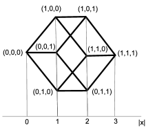
Figure 1: The hypercube in $n=3$ dimensions. The Hamming weight $\left|\vec{x}\right|$ measures the distance between $\vec{x}$ and $\vec{0}$. To illustrate this, all vertices with the same Hamming weight are projected to one point.

We now employ this quantum walk to construct a quantum search algorithm. We mark the target vertex $v$ with a different coin flip, that is, we choose a local coin matrix at $v$ with $C_{1}=-\mathbbm{1}_{n}$. The marked coin acting on the full Hilbert space is then given as

$$C^{\prime}=C-\left(C_{0}-C_{1}\right)\otimes\left|v\right\rangle\left\langle v\right|\,.$$ (6)

This defines a ‘perturbed’ quantum walk $U^{\prime}=SC^{\prime}$, which can be written as

$$U^{\prime}=U\left(\mathbbm{1}_{2^{n}n}-2\left|sv\right\rangle\left\langle sv\right|\right)\,,$$ (7)

where $\left|sv\right\rangle=\left|s\right\rangle\otimes\left|v\right\rangle$ is a state localised at the marked vertex and uniformly distributed in coin space. Note that $|sv\rangle$ is orthogonal to all trivial eigenvectors [12]. Eqn. (7) is obtained using the definition of $C_{0}$ and $C_{1}$, that is,

$$U^{\prime} = SC^{\prime}=SC-S\left(\left(C_{0}-C_{1}\right)\otimes\left|v\right\rangle\left\langle v\right|\right)$$ (8)

$$= SC-S\left(\left(2|s\rangle\langle s|-\mathbbm{1}_{n}+\mathbbm{1}_{n}\right)\otimes|v\rangle\langle v|\right)$$

$$= SC-2SC\left(|s\rangle\langle s|\otimes|v\rangle\langle v|\right)$$

$$= U\left(\mathbbm{1}_{2^{n}n}-2|sv\rangle\langle sv|\right),$$

where we use $C_{0}|s\rangle=|s\rangle$. The search algorithm is now started in the eigenstate $\left|v_{\vec{0}}\right\rangle$ of the unperturbed walk which is uniformly distributed over the whole Hilbert space, see Eqn. (3). It has been shown in [1] that the state $\left(U^{\prime}\right)^{t}|v_{\vec{0}}\rangle$ localises on the marked vertex after $t={\cal O}(\sqrt{N})$ steps with $N=2^{n}$, the total number of vertices. In what follows, we will present an alternative derivation of this result which provides additional insight into the localisation process and offers improved estimates for the localisation time.

3 Introduction of $U_{\lambda}$ and the reduced space ${\cal{H}}^{\prime}$

We first note that the operator $U^{\prime}$ is close to $U$ in the sense that we can write $U^{\prime}=U-2U\left|sv\right\rangle\left\langle sv\right|$. The additional term $2U\left|sv\right\rangle\left\langle sv\right|$ changes only a few entries in $U$. In fact, we can choose a basis where $U$ and $U^{\prime}$ are identical in all but one entry.

We may thus regard the additional term as a localised perturbation of $U$. In order to study how this perturbation effects the spectrum, we consider a family of operators $U_{\lambda}$ changing continuously from $U$ to $U^{\prime}$ as $\lambda$ is varied from 0 to 1. The following definition

$$U_{\lambda}=U\left(\mathbbm{1}_{2^{n}n}+\left({\rm e}^{{\rm i}\lambda\pi}-1\right)\left|sv\right\rangle\left\langle sv\right|\right)$$ (9)

fulfils this condition, that is, $U_{\lambda}$ is a continuous matrix valued function in $\lambda$ and equals $U$ and $U^{\prime}$ for $\lambda=0$ and $\lambda=1$, respectively. $U_{\lambda}$ is in addition periodic with period 2 and is unitary for all $\lambda$.

In order to understand the effect of the perturbation on the spectrum of $U^{\prime}$, we consider the symmetries of the hypercube; they can be described in terms of two types of symmetry operations, $P_{i}$ and $P_{ij}$ with $i,j=1,\ldots n$. Writing the set of vertices as $n$-digit strings containing $0$s and $1$s, $P_{i}$ is defined as the operation that flips the $i$th digit from $0\to 1$ or $1\to 0$, respectively, and $P_{ij}$ is the operator exchanging the $i$th and the $j$th digit. Note that $P_{i}$ changes the Hamming weight of the vertex whereas $P_{ij}$ does not. The group of symmetry operations on the hypercube is generated by $P_{i}$ and $P_{ij}$. Both operators represent reflections at an $n-1$ dimensional manifold orthogonal to $\vec{e}_{i}$ and $\vec{e}_{i}-\vec{e}_{j}$ respectively, where $\vec{e}_{i}$ is defined as the unit vector pointing in the $i$th direction.

Let us assume that the marked vertex sits at $v=\vec{o}$. Such a perturbation breaks all symmetries created by $P_{i}$. The marked vertex (with coin $C_{1}$) is, however, at a fixed point of $P_{ij}$ and the corresponding symmetries are not affected by the perturbation. As a result, not all symmetries of the unperturbed spectrum are lifted and the analysis can be done in a symmetry reduced space.

In particular, all eigenvectors of $U$ orthogonal to $\left|sv\right\rangle$ are also eigenvectors of $U_{\lambda}$ and their corresponding eigenvalues remain unchanged when varying $\lambda$ in (9). Since these eigenvectors are not affected by the perturbation introduced by the marked vertex, we concentrate our investigation on eigenvectors that are not orthogonal to $\left|sv\right\rangle$. We reorganise the eigenvectors such that there is only one eigenvector in each degenerate eigenspace which is not orthogonal to $\left|sv\right\rangle$. These vectors are given by $\left|\omega^{\pm\prime}_{k}\right\rangle=\sum_{\vec{l},\left|\vec{l}\right|=k}\left|v^{\pm}_{\vec{l}}\right\rangle\left\langle v^{\pm}_{\vec{l}}\mid sv\right\rangle$ which after normalisation yields

$$\left|\omega^{\pm}_{k}\right\rangle:=\frac{1}{\sqrt{n\choose k}}\sum_{\vec{l}\atop\left|\vec{l}\right|=k}\left(-1\right)^{\vec{l}\cdot\vec{v}}\left|v^{\pm}_{\vec{l}}\right\rangle,$$ (10)

where $\vec{v}$ are the coordinates of the marked vertex $v$; this definition is not independent of $v$. In the following, we will assume that the marked vertex is at $\vec{0}$. We discuss the general case in Sec. 8. We then obtain

$$\left|\omega^{\pm}_{k}\right\rangle=\frac{1}{\sqrt{n\choose k}}\sum_{\vec{l}\atop\left|\vec{l}\right|=k}\left|v^{\pm}_{\vec{l}}\right\rangle$$ (11)

as the set of $2n$ normalised eigenvectors of $U$ containing the marked vertex $v$. These vectors span a $2n$-dimensional subspace ${\cal{H}}^{\prime}$ of the full Hilbert space [1]. Note, that the marked state $\left|sv\right\rangle$ is in ${\cal{H}}^{\prime}$ and that the trivial eigenvectors are orthogonal to $\left|sv\right\rangle$ [12]. Thus, ${\cal{H}}^{\prime}$ is mapped onto itself under the map $U_{\lambda}$. That implies, that the definition of $U_{\lambda}$ in Eqn. (12) holds for the reduced space,

$$U_{\lambda}=U\left(\mathbbm{1}_{2{n}}+\left({\rm e}^{{\rm i}\lambda\pi}-1\right)\left|sv\right\rangle\left\langle sv\right|\right)$$ (12)

where $U$, $U_{\lambda}$ are the quantum walks restricted to the reduced space in the basis (11).

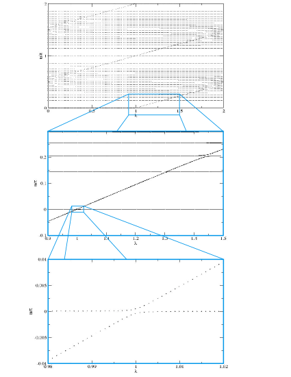
Figure 2: Phases of the eigenvalues of $U_{\lambda}$ in units of $\pi$ as a function of $\lambda$ for a $20$ dimensional hypercube in the reduced space.

4 Spectrum of $U_{\lambda}$

We start by describing main features of the spectrum of $U_{\lambda}$. Fig. 2 shows the eigenphases of the unitary matrix $U_{\lambda}$ as a function of $\lambda$ in the $2n$ dimensional reduced space ${\cal{H}}^{\prime}$. To simplify notation, we define a new index $m$ replacing $k$ and $\pm$ such that $m\in\{-n+1,n\}$ and $\{k,\pm\}=\{\left|m\right|,{\rm sgn}\left(m\right)\}$. We furthermore write the eigenvalues and eigenvectors as ${\rm e}^{\pm{\rm i}\omega_{k}}={\rm e}^{{\rm i}\omega_{m}}$ and $\left|\omega_{k}^{\pm}\right\rangle=\left|\omega_{m}\right\rangle$, respectively.

The numerical results indicate that the eigenphases $\omega_{m}$ of the unperturbed walk, corresponding to $\lambda=0$ or 2 and given in Eqn. (2), remain largely unchanged when changing $\lambda$. In addition, there are “perturber” states with eigenphases roughly parallel to the line $\frac{\pi}{2}\lambda$. One finds avoided crossings at points where the eigenphases related to $\omega_{m}$ ‘cross’ the perturber states. In the following we will concentrate on the perturber state $|u_{\lambda}\rangle$ causing an avoided crossing at $\omega=0$ and $\lambda=1$; this is called the $m=0$-th crossing.

The dynamics at an avoided crossing can essentially be described in terms of a two level system where the interaction induced by the map $U_{\lambda}$ between the states at the crossing is much larger than that with any of the other unperturbed eigenstates. At the $m$-th crossing at $\lambda=\lambda_{m}$, say, we can construct a two-level dynamics between the unperturbed eigenvector $|\omega_{m}\rangle$ given in (11) and a perturber state $|u_{m}\rangle$ to be determined below. These two states have a large overlap with the exact eigenvectors $|w_{m}^{\pm}\rangle$ at $\lambda=\lambda_{m}$. We can in fact write the eigenvectors in good approximation as $|w_{m}^{\pm}\rangle\approx(|\omega_{m}\rangle\pm|u_{m}\rangle)/\sqrt{2}$ for a suitable choice of phases.

Performing the walk in the two dimensional subspace spanned by $\left|\omega_{m}\right\rangle$ and $\left|u_{m}\right\rangle$ makes it possible to rotate the start state $\left|\omega_{m}\right\rangle$ into the target state $\left|u_{m}\right\rangle$. The latter has a large overlap with the state of the marked vertex $\left|sv\right\rangle$ and its nearest neighbours. (It will be shown that $\left\langle sv\mid u_{m}\right\rangle\approx 2^{-1/2}$).

The time it takes to perform the rotation from $\left|\omega_{m}\right\rangle$ to $\left|u_{m}\right\rangle$ by applying $U_{\lambda}$ at $\lambda=\lambda_{m}$ is determined by the gap $\Delta_{m}$ between the two levels at the $m$-th avoided crossing. One finds

$$U^{t}_{\lambda_{m}}\left|\omega_{m}\right\rangle = \frac{1}{\sqrt{2}}\left({\rm e}^{{\rm i}t\left(\omega_{m}+\frac{\Delta_{m}}{2}\right)}\left|w_{m}^{+}\right\rangle+{\rm e}^{{\rm i}t\left(\omega_{m}-\frac{\Delta_{m}}{2}\right)}\left|w_{m}^{-}\right\rangle\right)\,.$$ (13)

When choosing the time $t=T_{m}$, such that ${\rm e}^{{\rm i}T_{m}\frac{\Delta_{m}}{2}}={\rm i}$, that is,

$$T_{m}=\frac{\pi}{\Delta_{m}}\,,$$ (14)

we have

$$U^{T_{m}}_{\lambda_{m}}\left|\omega_{m}\right\rangle={\rm e}^{{\rm i}T_{m}\omega_{m}}{\rm i}\left|u_{m}\right\rangle\,.$$ (15)

In practise, $T_{m}$ is the nearest integer to $\frac{\pi}{\Delta_{m}}$. This procedure is very much in analogy to Grover’s algorithm [2, 3] except that the relation between the exact eigenstates and the start and target states is only an approximation here. Note, that increasing the gap $\Delta_{m}$ leads to a speed up of the search.

The quantum search algorithm [1] works at $\lambda=1$, that is, at the $m=0$ crossing starting with the initial distribution $\left|\omega_{0}\right\rangle$; it localises at the marked vertex after ${\cal O}(\sqrt{N})$ time steps where $N=2^{n}$ is the number of vertices of the hypercube. Note that $\left|\omega_{0}\right\rangle$ corresponds to the uniform distribution in the full space. The quantum walk for $n=12$ and $m=0$ is shown in Fig. 3 starting on $\left|\omega_{0}\right\rangle$. One clearly sees a strong localisation at the marked vertex $|0\rangle$ after roughly $70$ steps.

The origin of the gap is discussed at length in [1] ; we see here that it emerges through an avoided crossing. In fact, every avoided crossing can potentially be exploited as a search algorithm in the reduced space.

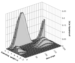
Figure 3: Performance of the search algorithm. The search algorithm on the $n=12$ dimensional hypercube in the reduced space; (all vertices with the same Hamming weight merge into one point). At $t=0$ the walk starts in the state $|\omega_{0}\rangle$ corresponding to the uniform distribution in the full space and localises at the marked vertex $v=\vec{0}$ at $t=74$.

5 Approximate eigenvectors and eigenvalues of $U_{\lambda}$

We will now derive an approximation for the perturber state $|u_{\lambda}\rangle$ as well as the spectral gaps $\Delta_{m}$. Starting from the definition of $U_{\lambda}$ and $|\omega_{m}\rangle$ in Eqs. (11), (12), one obtains for

$$U_{\lambda}\left|\omega_{m}\right\rangle={\rm e}^{i\omega_{m}}\left|\omega_{m}\right\rangle+\left({\rm e}^{{\rm i}\lambda\pi}-1\right)\beta_{m}\sqrt{n\choose|m|}2^{-n/2-1/2}{\rm e}^{\varphi_{m}}U\left|sv\right\rangle,$$ (16)

where ${\rm e}^{\pm{\rm i}\varphi_{k}}=\frac{\sqrt{k}\pm{\rm i}\sqrt{n-k}}{\sqrt{n}}\equiv{\rm e}^{{\rm i}\varphi_{m}}$ and $\beta_{m}$ is given in (5). Thus, $\left|\omega_{m}\right\rangle$ is already an approximate eigenvector of $U_{\lambda}$ with exponentially small remainder term of the order ${\cal O}(2^{-n/2})$ for $m$ close to $0$ or $n$. The eigenvalues of these vectors correspond to the horizontal lines in Fig. 2

We now come to the construction of the perturber state $|u_{\lambda}\rangle$; let $g\left(\lambda\right)$ be the eigenphase of the perturber state, that is, the eigenvalues of $U_{\lambda}$ are $\pm{\rm e}^{{\rm i}g\left(\lambda\right)}$. We expect that $g(\lambda)$ is roughly given by $g\left(\lambda\right)\approx\left(\lambda-1\right)\frac{\pi}{2}$. We set

$$\left|u_{\lambda}\right\rangle=2^{-n/2-1}\sum_{m=-n+1}^{n}\sqrt{n\choose|m|}{\rm e}^{{\rm i}\varphi_{m}}\beta_{m}a_{m}\left|\omega_{m}\right\rangle$$ (17)

for some yet unknown set of coefficients $a_{m}$. Writing $\left|sv\right\rangle$ in the $\left|\omega_{m}\right\rangle$-basis, one finds

$$\left|sv\right\rangle=2^{-n/2-1/2}\sum_{m=-n+1}^{n}\sqrt{n\choose|m|}{\rm e}^{{\rm i}\varphi_{m}}\beta_{m}\left|\omega_{m}\right\rangle.$$ (18)

The scalar product $\left\langle sv\mid u_{\lambda}\right\rangle$ gives

$$\left\langle sv\mid u_{\lambda}\right\rangle=2^{-n-3/2}b,$$ (19)

where $b$ is defined as

$$b=\sum_{m=-n+1}^{n}{n\choose|m|}a_{m}\beta_{m}^{2}.$$ (20)

The aim is to construct $\left|u_{\lambda}\right\rangle$ such that $U_{\lambda}\left|u_{\lambda}\right\rangle={\rm e}^{{\rm i}g\left(\lambda\right)}\left|u_{\lambda}\right\rangle$. Using the representation (17), we obtain

$$U_{\lambda}\left|u_{\lambda}\right\rangle = U\left|u_{\lambda}\right\rangle+\left({\rm e}^{{\rm i}\lambda\pi}-1\right)U\left|sv\right\rangle\left\langle sv\mid u_{\lambda}\right\rangle$$ (21)

$$= {\rm e}^{{\rm i}g\left(\lambda\right)}\left|u_{\lambda}\right\rangle+2^{-n/2-1}\sum_{m=-n+1}^{n}\sqrt{n\choose|m|}{\rm e}^{{\rm i}\varphi_{m}}\beta_{m}\left|\omega_{m}\right\rangle$$

$$\left[\left(-{\rm e}^{{\rm i}g\left(\lambda\right)}+e^{{\rm i}\omega_{m}}\right)a_{m}+\left({\rm e}^{{\rm i}\lambda\pi}-1\right)2^{-n-1}e^{{\rm i}\omega_{m}}b\right].$$

We can thus choose

$$a_{m}=\frac{\left(1-{\rm e}^{{\rm i}\lambda\pi}\right)2^{-n-1}b\,{\rm e}^{{\rm i}\omega_{m}}}{{\rm e}^{{\rm i}\omega_{m}}-{\rm e}^{{\rm i}g\left(\lambda\right)}}\,,$$ (22)

so that the second part of Eqn. (21) vanishes. Note that $b$ still depends on the coefficients $a_{m}$ and Eqn. (22) represents thus a homogeneous set of coupled linear equations. A solution of this set of equations exists only if the determinant of the coefficient matrix vanishes. Inserting (22) in (20) we may write this condition in terms of a ‘sum rule’

$$\frac{2^{n+1}}{1-{\rm e}^{{\rm i}\lambda\pi}}=\sum_{m=-n+1}^{n}{n\choose|m|}\frac{\beta_{m}^{2}{\rm e}^{{\rm i}\omega_{m}}}{{\rm e}^{{\rm i}\omega_{m}}-{\rm e}^{{\rm i}g\left(\lambda\right)}},$$ (23)

which implicitly defines the eigenphases $g(\lambda)$. The coefficient $b$ thus remains undetermined. So far, we have only rewritten the eigenvalue equation and we thus expect $n$ different solutions for $g(\lambda)$ for every value of $\lambda$. Note, that the singular behaviour whenever $\omega_{m}\approx g(\lambda)$ indicates that the corresponding coefficient $a_{m}$ dominates the expansion (except near an avoided crossing or for the perturber states).

For the corresponding eigenvector, we find

$$\left|u_{\lambda}\right\rangle = 2^{-n/2-1}\sum_{m=-n+1}^{n}\sqrt{n\choose|m|}{\rm e}^{{\rm i}\varphi_{m}}a_{m}\left|\omega_{m}\right\rangle$$ (24)

$$= b\,2^{-\frac{3}{2}n-2}\left(1-{\rm e}^{{\rm i}\lambda\pi}\right)\sum_{m=-n+1}^{n}\sqrt{n\choose|m|}\frac{{\rm e}^{{\rm i}\varphi_{m}+{\rm i}\omega_{m}}\beta_{m}}{{\rm e}^{{\rm i}\omega_{m}}-{\rm e}^{{\rm i}g\left(\lambda\right)}}\left|\omega_{m}\right\rangle,$$

and we identify $b$ as a normalisation constant. Note, that the vector $\left|u_{\lambda}\right\rangle$ coincides with the basis vectors $\left|\omega_{m}\right\rangle$ for $\lambda=2j$, $j\in\mathbbm{Z}$ and $g(\lambda)\approx\omega_{m}$.

We are here mostly interested in finding the states forming the two level system at an avoided crossing. The corresponding eigenspace at the $m$-th crossing will be spanned by the unperturbed eigenstate $\left|\omega_{m}\right\rangle$ (which is already exponentially close to the true eigenvalue, see (16)) and a second approximate eigenvector. This second vector may be found by defining a local vector near the $m$-th crossing $\left|u_{m}\right\rangle$ orthogonal to $\left|\omega_{m}\right\rangle$; we set

$$\left|u_{m}\right\rangle=b\,2^{-\frac{3}{2}n-2}\left(1-{\rm e}^{{\rm i}\lambda\pi}\right)\sum_{l=-n+1\atop l\neq m}^{n}\sqrt{n\choose|l|}\frac{{\rm e}^{{\rm i}\varphi_{l}+{\rm i}\omega_{l}}\beta_{l}}{{\rm e}^{{\rm i}\omega_{l}}-{\rm e}^{{\rm i}g\left(\lambda\right)}}\left|\omega_{l}\right\rangle.$$ (25)

If $b\ll 2^{3/2n}$, we can assume that the neglected term is small and $\left|u_{m}\right\rangle$ is a good local approximation to the true eigenvalue. An estimate for $b$ verifying this assumption will be given below.

The compatibility condition (23) then takes on the form of a local sum rule (setting $a_{l}=0$),

$$\frac{2^{n+1}}{1-{\rm e}^{{\rm i}\lambda\pi}}=\sum_{l=-n+1\atop l\neq m}^{n}{n\choose|l|}\frac{{\rm e}^{{\rm i}\omega_{l}}\beta_{l}^{2}}{{\rm e}^{{\rm i}\omega_{l}}-{\rm e}^{{\rm i}g\left(\lambda\right)}}.$$ (26)

We can use (26) to obtain local approximations of the phase $g(\lambda)$ near the $m$-th crossing. We will concentrate here on the main crossing at $\lambda=1$ for $m$=0. Neglecting interaction with the unperturbed state $\left|\omega_{0}\right\rangle$ (taken into account in the next section), we set ${\rm e}^{{\rm i}g\left(1\right)}=1$ at the crossing, that is, we demand $g\left(1\right)=0$.

We will show that

$$S(\lambda):=\frac{1-{\rm e}^{{\rm i}\pi\lambda}}{2^{n+1}}\sum_{l=-n+1\atop l\neq 0}^{n}{n\choose|l|}\frac{{\rm e}^{{\rm i}\omega_{l}}\beta_{l}^{2}}{{\rm e}^{{\rm i}\omega_{l}}-{\rm e}^{{\rm i}g\left(\lambda\right)}}=1+{\cal O}(e^{-n})$$ (27)

at $\lambda=1$, that is, Eqn. (26) is fulfilled up to an exponentially small error term.

Using that the spectrum is symmetric with respect to $0$, that is, for every $l\in[-n+1,n]$ there exists one $k\in[-n+1,n]$ such that ${\rm e}^{{\rm i}\omega_{k}}=-{\rm e}^{{\rm i}\omega_{l}}$ and writing $S(\lambda)$ in terms of $\omega_{l}\in(0,\pi)$ only, we obtain

$$S(\lambda)=\frac{1-{\rm e}^{{\rm i}\pi\lambda}}{2^{n}}\sum_{l=1}^{n-1}{n\choose l}\frac{{\rm e}^{2{\rm i}\omega_{l}}}{{\rm e}^{2{\rm i}\omega_{l}}-{\rm e}^{{\rm i}2g\left(\lambda\right)}}+\frac{1-{\rm e}^{{\rm i}\pi\lambda}}{2^{n+1}}.$$ (28)

Using $\sum_{l=0}^{n}{n\choose l}=2^{n}$, we may write

$$S(\lambda) = \frac{1-{\rm e}^{{\rm i}\pi\lambda}}{2^{n+1}}\left[2^{n}-1-{\rm i}\sum_{l=1}^{n-1}{n\choose l}\cot\left(\omega_{l}-g\left(\lambda\right)\right)\right].$$ (29)

Setting $g\left(1\right)=0$, we find $S(1)=1+2^{-n}$. By expanding $S(\lambda)$ in a power series in $\lambda$ and demanding that the derivatives of $S(\lambda)$ vanish at $\lambda=1$, we obtain conditions for the derivatives of $g\left(\lambda\right)$; in particular, one finds,

$$g^{\prime}\left(1\right)=\frac{\pi}{2\left(1+\gamma_{n}-2^{-n+1}\right)}$$ (30)

with

$$\gamma_{n}=\frac{1}{2^{n}}\sum_{l=1}^{n-1}{n\choose l}\cot^{2}(\omega_{l})\sim\frac{1}{n}\quad\mbox{for large }n.$$ (31)

The last estimate is obtained asymptotically by using the de Moivre-Laplace theorem and Poisson summation. Note, that for $n\rightarrow\infty$, this result coincides with $g\left(\lambda\right)\approx(\lambda-1)\pi/2$ as stated in the beginning of the section. Similarly, we can construct functions $g(\lambda)$ at crossings $m\neq 0$.

From Eqn. (26), we determine the normalisation constant $b$ by writing

$$1 = \left\langle u_{m}\mid u_{m}\right\rangle$$ (32)

$$= \left|b\right|^{2}2^{-3n-4}\left|1-{\rm e}^{{\rm i}\pi\lambda}\right|^{2}\sum_{l=-n+1\atop l\neq m}^{n}{n\choose|l|}\frac{\beta_{l}^{2}}{\left|{\rm e}^{{\rm i}\omega_{l}}-{\rm e}^{{\rm i}g\left(\lambda\right)}\right|^{2}}$$

and thus

$$\frac{1}{\left|b\right|^{2}} = 2^{-3n-4}\left|1-{\rm e}^{{\rm i}\pi\lambda}\right|^{2}\sum_{l=-n+1\atop l\neq m}^{n}{n\choose|l|}\frac{\beta_{l}^{2}}{\left|{\rm e}^{{\rm i}\omega_{l}}-{\rm e}^{{\rm i}g\left(\lambda\right)}\right|^{2}}\,.$$ (33)

The sum can be calculated using Eqn. (26) (and neglecting exponentially small terms). The derivative of (26) with respect to $\lambda$ leads to

$$\frac{\pi}{g^{\prime}\left(\lambda\right)}\frac{2^{n+1}}{\left|1-{\rm e}^{{\rm i}\lambda\pi}\right|^{2}}=\sum_{l=-n+1\atop l\neq m}^{n}{n\choose|l|}\frac{\beta_{l}^{2}}{\left|{\rm e}^{{\rm i}\omega_{l}}-{\rm e}^{{\rm i}g\left(\lambda\right)}\right|^{2}},$$ (34)

and hence $\left|b\right|^{2}=\frac{2g^{\prime}\left(\lambda\right)}{\pi}2^{2n+2}$. We are free to choose a phase for the vector $|u_{m}\rangle$ and set

$$b:=\sqrt{\frac{2g^{\prime}\left(\lambda\right)}{\pi}}2^{n+1}.$$ (35)

Therefore the condition $b\ll 2^{3n/2}$ stated after Eqn. (25) is fulfilled for large $n$ and $\left|u_{m}\right\rangle$ is an approximative eigenvector of $U_{\lambda}$.

6 Matrix elements of $U_{\lambda}$.

To calculate the size of the gap $\Delta_{m}$ between the two eigenvalues at the $m$-th avoided crossing, we consider how $U_{\lambda}$ acts on the $2\times 2$ space spanned by $|\omega_{m}\rangle$ and $|u_{m}\rangle$. At the $m$th crossing, we find $\lambda=\lambda_{m}=g^{-1}\left(\omega_{m}\right)$ and the corresponding matrix elements of $U_{\lambda}$ are

$$A := \left\langle u_{m}\mid U_{\lambda_{m}}\mid u_{m}\right\rangle={\rm e}^{{\rm i}g\left(\lambda_{m}\right)}$$

$$B := \left\langle\omega_{m}\mid U_{\lambda_{m}}\mid u_{m}\right\rangle$$

$$= 2^{-n/2-1}\left({\rm e}^{{\rm i}\lambda_{m}\pi}-1\right){\rm e}^{{\rm i}\omega_{m}+{\rm i}\varphi_{l}}\sqrt{{n\choose|m|}}\beta_{m}\sqrt{\frac{2g^{\prime}\left(\lambda\right)}{\pi}}$$

$$C := \left\langle u_{m}\mid U_{\lambda_{m}}\mid\omega_{m}\right\rangle$$

$$= -2^{-n/2-1}\left({\rm e}^{-{\rm i}\lambda_{m}\pi}-1\right){\rm e}^{{\rm i}g\left(\lambda_{m}\right)-{\rm i}\varphi_{m}}\sqrt{{n\choose|m|}}\beta_{m}\sqrt{\frac{2g^{\prime}\left(\lambda\right)}{\pi}}$$

$$D := \left\langle\omega_{m}\mid U_{\lambda_{m}}\mid\omega_{m}\right\rangle={\rm e}^{{\rm i}\omega_{m}}\left(1+\left({\rm e}^{{\rm i}\lambda_{m}\pi}-1\right)2^{-n-1}\beta_{m}^{2}{n\choose|m|}\right).$$

The $2\times 2$ matrix $W=\begin{pmatrix}A&B\\ C&D\end{pmatrix}$ characterises the avoided crossings in $U_{\lambda}$ to a good approximation. Note that we have $|A|\sim|D|\sim 1$ and $|B|\sim|C|\sim\sqrt{{n\choose|m|}}e^{-n/2-1}\ll 1$ for small $m/n$.

The gap $\Delta_{m}$ in the spectrum is given by the difference of the two eigenphase; for small differences, this is in leading order given by the difference between the two eigenvalues of $W$.

We thus obtain

$$\Delta_{m}^{2} := \left(D-A\right)^{2}+4BC$$ (36)

$$= \left({\rm e}^{{\rm i}\omega_{m}}-{\rm e}^{{\rm i}g\left(\lambda_{m}\right)}+2^{-n-1}{n\choose|m|}\beta_{m}^{2}\left({\rm e}^{{\rm i}\lambda_{m}\pi}-1\right){\rm e}^{{\rm i}\omega_{m}}\right)^{2}$$

$$-2^{-n}\left|1-{\rm e}^{{\rm i}\lambda_{m}\pi}\right|^{2}{n\choose|m|}{\rm e}^{{\rm i}g\left(\lambda_{m}\right)+{\rm i}\omega_{m}}\beta_{m}^{2}\,\frac{2g^{\prime}\left(\lambda\right)}{\pi}\,.$$

By construction, we have $g\left(\lambda_{m}\right)=\omega_{m}$ at the crossing, and thus

$$\left|\Delta_{m}\right|=\left|1-{\rm e}^{{\rm i}\lambda_{m}\pi}\right|2^{-n/2}\sqrt{n\choose|m|}\beta_{m}\sqrt{\frac{2g^{\prime}\left(\lambda\right)}{\pi}}+{\cal O}\left(2^{-n}{n\choose|m|}\right),$$ (37)

neglecting terms of the order $2^{-n}$ both in the matrix elements and in the ’sum rule’ (27).

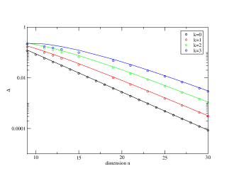
Figure 4: Comparison of numerical and theoretical values for the size of the gap. The circles correspond to numerical results while the solid lines correspond to the theoretical results given by $2^{-n/2}\sqrt{{n\choose|m|}}\left|1-{\rm e}^{{\rm i}\lambda_{m}\pi}\right|$ for several values $m$ as a function of the dimension $n$.

In Fig. 4 we compare the leading order term, Eqn. (37), with numerical results for the first four crossings as a function of the dimension of the hypercube. Clearly, our estimate captures the behaviour of the gap very well, even at intermediate values of $n$ down to $n\approx 10-15$. We note in particular that the size of the gap increases with the order of the crossing $|m|$.

7 Time of the search

The quantum algorithm takes place in the two dimensional subspace spanned by the two approximate eigenvectors involved in the avoided crossing, $\left|\omega_{m}\right\rangle$ and $\left|u_{m}\right\rangle$. In analogy to Grover’s algorithm [2, 3], the search corresponds to a rotation from an initial state $|\omega_{m}\rangle$ to a final state localised at the marked item and its nearest neighbours; see the discussion in Sec. 4. Direct calculation using (19) and (35) yields,

$$\left\langle u_{m}\mid sv\right\rangle\approx 2^{-1/2}\sqrt{2g^{\prime}\left(\lambda\right)/\pi}\approx\left|\left\langle u_{m}\mid U\mid sv\right\rangle\right|,$$ (38)

where $\sqrt{2g^{\prime}\left(0\right)/\pi}\approx 1$ for large $n$ and we approximate $u_{\lambda}$ by $u_{m}$ at the crossing. That is, the target state $\left|u_{m}\right\rangle$ has a large overlap with the marked vertex $|sv\rangle$ or its immediate neighbours, $U|sv\rangle$. Any measurement will thus yield with a high probability either $|sv\rangle$ or one of its neighbouring vertices when done after $T_{m}$ time steps. This implies, that we can define a quantum search algorithm for every avoided crossing $m$ (as long as the dynamics effectively takes place in a two-level system). The search time $T_{m}$ is given by Eqn. (14), that is

$$T_{m}=\frac{\pi 2^{n/2}\sqrt{\frac{\pi}{2g^{\prime}\left(\lambda_{m}\right)}}}{\left|1-{\rm e}^{{\rm i}\lambda_{m}\pi}\right|\sqrt{n\choose|m|}\beta_{m}}.$$ (39)

In particular, the $T_{m}$ decreases with increasing $m$ thus making search algorithms at higher order crossings potentially more effective.

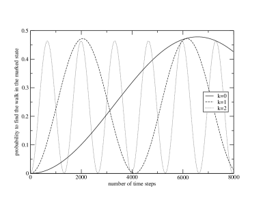
Figure 5: The probability to measure the state at the marked vertex in $n=25$ dimensions for the central crossing $m=0$ and the first ancillary crossings $m=1$ and $m=2$.

Fig. 5 shows the probability to measure the quantum walk in the reduced space at the marked vertex as a function of time and $n=25$. It is evident from the figure, that the quantum search localises on the marked vertex with a 50% probability for all algorithms shown (corresponding here to the crossings $m=0,1,2$). In particular, the search becomes faster with increasing $m$ in accordance with (39). For the search algorithm for $m=2$, we find the marked vertex in $1/10$th of the time compared to a search with $m=0$ and only a small loss in amplitude. If we proceed to higher $m$, one looses more and more amplitude and the search becomes inefficient; in our example ($n=25$) this happens for $m>4$. In general, we find that the quantum search algorithm fails to localise at the marked vertex when the gap is of the size of the distance between two adjacent (unperturbed) eigenvalues.

8 Results in the original space $\cal H$ for general $v$

The class of search algorithms considered in the previous section act in the reduced space finding the marked vertex in ${\cal O}\left(\sqrt{N}\right)$ time. To start the search, one needs to know the parameter values $\lambda_{m}$ and the initial state $|\omega_{m}\rangle$. The former can in principle be obtained to arbitrary accuracy for a given dimension $n$ or are known explicitly as in the case $m=0$. The starting vectors $|\omega_{m}\rangle$ defined in Eqn. (10) depend, however, on the choice of the marked vertex $v$ for $m\neq 0$. In fact, the reduction of the space itself as described in Sec. 3 is not independent of the marked vertex; when simplifying Eqn. (10) to Eqn. (11), we explicitly put the marked vertex at $v=\vec{0}$. Any other choice of $v$ will, however, change the starting vectors $|\omega_{m}\rangle$ for $m\neq 0$ or equivalently change the point of origin for the symmetry operations $P_{i}$, $P_{ij}$ (see Sec., 3).

We are ultimately interested in search algorithms on the full hypercube. This can be achieved directly by employing the $m=0$ crossing. The corresponding initial vector $|\omega_{0}\rangle$ is independent of $v$ with $\lambda_{0}=1$; this yields the search algorithm in [1]. It is, however, the slowest algorithm of the ones discussed in the previous section. To make use of any of the other search algorithms, we need the starting vector $|\omega_{m}\rangle$ given in Eqn. (10), which depends, however, on the marked vertex itself.

This optimal starting vector is embedded in the ${n\choose|m|}$ dimensional vector space related to the eigenvalue $m$ in the unperturbed space $\cal{H}$. This space is spanned by the vectors $|v_{\vec{k}}^{\pm}\rangle$, (where $\pm|\vec{k}|=m$), given in Eqn. (3). So, in addition to finding the marked vertex, one also needs to search for the state $|\omega_{m}\rangle$. We have not succeeded in devising an efficient method for finding this optimal starting vector for arbitrary $v$, that is, a method that would not wipe out any gains made by improving the search time $T_{m}$ in Eqn. (39).

We conclude that the algorithms introduced above have search times which are all of the same order in the reduced space; only the original algorithm devised in [1] is, however, useful for searches on the full hypercube as no extra efforts are needed in finding both the values for $\lambda_{m}$ andi, more importantly, the optimal starting vector $|\omega_{m}\rangle$. The technique presented here provides an improved estimate for the search time and offers a new point of view by studying quantum random walks in terms of avoided crossings.
Acknowledgements:
We thank Fritz Haake and Brian Winn for carefully reading the manuscript and for valuable comments.

References

• [1] N Shenvi, J Kempe and K B Whaley: Quantum random-walk search algorithm Physical Review A, 67 052307 (2003).
• [2] L Grover: A fast quantum mechanical algorithm for database search in Proc. 28th STOC, ACM Press, Philadelphia, Pennsylvania, p.Β 212 (1996); L K Grover, Quantum mechanics helps in searching for a needle in a haystack Physical Review Letters, 97 325 (1997).
• [3] M A Nielsen and I L Chuang, Quantum Computation and Quantum Information Cambridge University Press (2000).
• [4] J Kempe: Quantum random walks - an introductory overview, Contemporary Physics, 44 307 (2003)
• [5] A Ambainis, Quantum walks and their algorithmic applications, International Journal of Quantum Information, 1 507, (2003).
• [6] S Gnutzmann and U Smilansky, Quantum Graphs: Applications to quantum chaos and universal spectral statistics, Advances in Physics 55, 527 (2006).
• [7] SΒ Severini and GΒ Tanner, Regular Quantum Graphs, J.Β Phys.Β A 37 6675 (2004).
• [8] G Tanner: From quantum graphs to quantum random walks in Non-Linear Dynamics and Fundamental Interactions Springer, Dordrecht, p 69 (2006).
• [9] S Aaronson and A Ambainis, Quantum search of spatial regions, Proc. 44th Annual IEEE Symp.Β on Foundations of Computer Science (FOCS), p.Β 200 (2003).
• [10] A Ambainis, J Kempe and A Rivosh: Coins make quantum walks faster Proc. 16th ACM-SIAM SODA, p.Β 1099 (2005)
• [11] A M Childs and J Goldstone, Spatial search by quantum walk Physical Review E, 70 022314 (2004).
• [12] C Moore and A Russell, in Proceedings of RANDOM, 2002, edited by J D P Rolim and P Vadham, Springer, Cambridge, MA, p.Β 164, (2002).