Renormalization and conjugacy of piecewise linear Lorenz maps

Abstract.

For each piecewise linear Lorenz map that expand on average, we show that it admits a dichotomy: it is either periodic renormalizable or prime. As a result, such a map is conjugate to a $\beta$-transformation.

1. Introduction

Lorenz maps are one-dimensional maps with a single discontinuity, which arise as Poincaré return maps for flows on branched manifolds that model the strange attractors of Lorenz systems. More precisely, $f:I\to I$ is a Lorenz map if there is a point $c$ in the interior of the interval $I$ and $f$ is continuous and increasing on both sides of $c$, and $f(\{c_{-},\ c_{+}\})\to\partial I$, where $f(c_{+})$ and $f(c_{-})$ are the one side limits of $f$ at $c$. We are interested with piecewise linear Lorenz maps of the form

(1) $$f_{a,b,c}(x)=\left\{\begin{array}[]{ll}ax+1-ac&x\in[0,\ c)\\ b(x-c)&x\in(c,\ 1].\end{array}\right.$$

The average slope of $f_{a,b,c}$ is $\int f^{\prime}_{a,b,c}(x)dx=ac+b(1-c)$. We say that $f_{a,b,c}$ expand on average if the average slope $ac+b(1-c)$ is greater than $1$. It is easy to see that the average slope is greater than $1$ if and only if $f_{a,b,c}(0)<f_{a,b,c}(1)$. We are concerned with the renormalization and conjugacy of piecewise linear Lorenz map that expand on average. Denote by $\mathcal{L}$ as the set of piecewise linear Lorenz maps that expand on average. Note that for $f_{a,b,c}\in\mathcal{L}$ we may have $a<1<b$ or $a>1>b$ because we only assume $ac+b(1-c)>1$. In both cases, $f_{a,b,c}$ is contractive on some interval.

The map $T_{\beta,\alpha}$ defined by

$$T_{\beta,\alpha}=\beta x+\alpha\ \ \ \mod 1$$

is called a $\beta$-transformation (see [9]). When $1<\beta\leq 2$, $0\leq\alpha<1$, $T_{\beta,\alpha}=f_{\beta,\beta,c}$ with $c=(1-\alpha)/\beta$.

The study of $\beta$-transformation goes back to R$\acute{e}$nyi. Based on bounded distortion principe, R$\acute{e}$nyi proved that $\beta$-transformation admits an acip (absolutely continuous invariant probability measure with respect to the Lebesgue measure). Gelfond [8] and Parry [17, 18] obtained the expression of the density of the acip. Flatto and Lagarias [5, 6, 7] studied the lap counting functions. For $f\in\mathcal{L}$, we proved in [3] that such a map admits an ergodic acip because there exists a positive integer $n$ so that $(f^{n}_{a,b,c})^{\prime}(x)>\lambda>1$ for all $x\in I$ except countable points. Such a map is expanding in the sense that $\cup_{n\geq 0}f^{-n}(c)$ is dense in $I$.

1.1. Renormalization of expanding Lorenz map

Renormalization is a central concept in contemporary dynamics. The idea is to study the small-scale structure of a class of dynamical systems by means of a renormalization operator $R$ acting on the systems in this class. This operator is constructed as a rescaled return map, where the specific definition depends essentially on the class of systems. A Lorenz map $f:I\to I$ is said to be renormalizable if there is a proper subinterval $[u,\ v]\ni c$ and integers $\ell,r>1$ such that the map $g:[u,\ v]\to[u,\ v]$ defined by

(2) $$g(x)=\left\{\begin{array}[]{ll}f^{\ell}(x)&x\in[u,\ c),\\ f^{r}(x)&x\in(c,\ v],\end{array}\right.$$

is itself a Lorenz map on $[u,\ v]$. The interval $[u,\ v]$ is called the renormalization interval. If $f$ is not renormalizable, it is said to be prime.

A renormalization $g=(f^{\ell},f^{r})$ of $f$ is said to be minimal if for any other renormalization $(f^{\ell^{\prime}},f^{r^{\prime}})$ of $f$ we have $\ell^{\prime}\geq\ell$ and $r^{\prime}\geq r$ (e.g. [11, 14]). It is not an easy problem to determine wether $f$ is renormalizable or not. In fact, it is impossible to check if $f$ is prime or not in finite steps, because $\ell$ and $r$ in (2) may be large.

The renormalization theory of expanding Lorenz maps is well understood (see for example, in [2, 11, 14]). We recall some results from [2] for completeness. Let $f$ be an expanding Lorenz map. A subset $E$ of $I$ is completely invariant under $f$ if $f(E)=f^{-1}(E)=E$, and it is proper if $E\neq I$. According to Theorem A in [2], there is a one-to-one correspondence between the renormalizations and proper completely invariant closed sets of $f$. In fact, let $E$ be a proper completely invariant closed set of $f$, put

(3) $$e_{-}=\sup\{x\in E:x<c\},\ \ \ \ \ e_{+}=\inf\{x\in E:x>c\},$$

$\ell$ and $r$ be the maximal integers so that $f^{\ell}$ and $f^{r}$ is continuous on $(e_{-},\ c)$ and $(c,\ e_{+})$, respectively. Then we have

(4) $$f^{\ell}(e_{-})=e_{-},\ \ \ \ f^{r}(e_{+})=e_{+},$$

and the map

(5) $$R_{E}f(x)=\left\{\begin{array}[]{ll}f^{\ell}(x)&x\in[f^{r}(c_{+}),\ c)\\ f^{r}(x)&x\in(c,\ f^{\ell}(c_{-})]\end{array}\right.$$

is a renormalization of $f$.

So a possible way to describe the renormalizability of $f$ is to look for the minimal completely invariant closed set of $f$. The minimal completely invariant closed set relates to the periodic orbit with minimal period of $f$. Suppose the minimal period of the periodic points of $f$ is $\kappa$. It is easy to see that $f$ is prime if $\kappa=1$ or $\kappa=\infty$. If $1<\kappa<\infty$, then $f$ admits unique $\kappa$-periodic orbit $O$. Put $D=\overline{\bigcup_{n\geq 0}f^{-n}(O)}$. Then we have the following statements (see Theorem B in [2]):

1. $D$ is the minimal completely invariant closed set of $f$.

2. $f$ is renormalizable if and only if $D\neq I$. If $f$ is renormalizable, then $R_{D}$, the renormalization associated to $D$, is the minimal renormalization of $f$.

3. We have the following trichotomy: i) $D=I$, ii) $D=O$, iii) $D$ is a Cantor set.

So the minimal renormalizaion of renormalizable expanding Lorenz map always exists. We can define a renormalization operator $R$ from the set of renormalizable expanding Lorenz maps to the set of expanding Lorenz maps ([2, 11]). For each renormalizable expanding Lorenz map, we define $Rf$ to be the minimal renormalization map of $f$. For $n>1$, $R^{n}f=R(R^{n-1}f)$ if $R^{n-1}f$ is renormalizable. And $f$ is $m$ ($0\leq m\leq\infty$) times renormalizable if the renormalization process can proceed $m$ times exactly. For $0<i\leq m$, $R^{i}f$ is the $i$th renormalization of $f$.

Definition 1.

Let $f$ be an expanding Lorenz map. The minimal renormalization is said to be periodic if the minimal completely invariant closed set $D=O$, where $O$ is the periodic orbit with minimal period of $f$. And the $i$th renormalization $R^{i}f$ is periodic if it is a periodic renormalization of $R^{i-1}f$.

The periodic renormalization is interesting because $\beta$-transformation can only be renormalized periodically (see [9]). This kind of renormalization was studied by Alsed$\grave{a}$ and Falc$\grave{o}$ [1], Malkin [13]. It was called phase locking renormalization in [1] because it appears naturally in Lorenz map whose rotational interval degenerates to a rational point.

Let $f$ be an expanding Lorenz map with a discontinuity $c$, $P_{L}$ be the largest $\kappa-$periodic point less than $c$ and $P_{R}$ be the smallest $\kappa-$periodic point greater than $c$. Then we have the following statements ([2]):

1. The minimal renormalization of $f$ is periodic if and only if

   (6) $$[f^{\kappa}(c_{+}),\ f^{\kappa}(c_{-})]\subseteq[f^{\kappa}(P_{L}),\ f^{\kappa}(P_{R})].$$

2. One can check if the minimal renormalization of $f$ is periodic or not in following steps:

   • Find the minimal period $\kappa$ of $f$ by considering the preimages of $c$, see Lemma 1;

   • Find the $\kappa$-periodic orbit;

   • Check if the inclusion (6) holds or not.

So the periodic renormalization in Lorenz map plays a similar role as the period-doubling renormalization in unimodal map.

1.2. Main result and ideas of proof

The main purpose of this note is to characterize the renormalizations of $f\in\mathcal{L}$.

Main Theorem. Let $f\in\mathcal{L}$, then each renormalization of $f$ is periodic. Furthermore, $f$ is conjugate to a $\beta$-transformation.

Follows from Milnor and Thurston [15], a Lorenz map $f$ is semi-conjugate to a $\beta$-transformation. According to Parry [19], $f$ is conjugate to a $\beta$-transformation if $f$ is strongly transitive. Since an expanding Lorenz map is strongly transitive if and only if it is prime [2], it is interesting to know when a renormalizable expanding Lorenz map is conjugate to a $\beta$-transformation.

Periodic renormalization is relevant to the conjugacy problem. Glendinning [9] showed that an expanding Lorenz map is conjugate to a $\beta$-transformation if its renormalizations admit some special forms. In our words, he obtained the following Proposition.

Proposition 1.

([9]) An expanding Lorenz map $f$ is conjugate to a $\beta$-transformation if and only if $f$ is finitely renormalizable and each renormalization of $f$ is periodic.

In fact, we shall actually prove the following Main Theorem’.

Main Theorem’. Let $f\in\mathcal{L}$, then $f$ is finitely renormalizable and each renormalization of $f$ is periodic.

Remark 1.

1. Main Theorem’ indicates that the renormalization process of $f\in\mathcal{L}$ is simple: all of the renormalizations are periodic. And one can obtain all of the renormalizations in finite steps.

2. Suppose $f\in\mathcal{L}$ is $m$-renormalizable, then by Theorem C in [2], $f$ admits a cluster of completely invariant closed sets

   $$\emptyset=E_{0}\subset E_{1}\subset E_{2}\subset\cdot\cdot\cdot\subset E_{m}\subset I,$$

   where $m$ is finite, and $E_{m-i}$ equals to the $ith$ derived set of $E_{m}$, $i=1,2,\ldots,m$.

3. According to Parry [20], when $a\in(2^{2^{-(m+1)}},\ 2^{2^{-m}}]$, the symmetric piecewise linear Lorenz map $f_{a,a,1/2}$ is $m$-renormalizable, so one can obtain countable set with given finite depth in dynamical way.

4. $f\in\mathcal{L}$, $E$ be a proper complete invariant closed set of $f$, and $g=R_{E}$ be the renormalization corresponds to $E$. Since $E$ is countable, the topological entropy $h(f|_{E})=0$ (cf. [2, 10, 12]). Such a renormalization does not induce phase transition under the natural potential $-t\log|Df|$ ([4]).

Let us point out the main ideas in the proof of our Main Theorem’. Denote by $\mathcal{LR}$ the class of maps in $\mathcal{L}$ which are renormalizable, and $\mathcal{L}_{2}$ be the class of maps in $\mathcal{L}$ and satisfy the additional condition

(7) $$(AC)\ \ \ \ \ \ \ \ \ \ \ \ \ \ \ \ \ 1-ac=f(0)<c<f(1)=b(1-c).\ \ \ \ \ \ \ \ \ \ \ \ \ \ \ \ \ \ \$$

According to Lemma 1 in Section 2, any map in $\mathcal{L}_{2}$ admits minimal period $\kappa=2$. Fix $f\in\mathcal{L}$, we denote $\kappa$ as its the minimal period, $O$ as the unique $\kappa$-periodic orbit and $D$ as the minimal completely invariant closed set of $f$.

Observe that $f\in\mathcal{LR}$ implies the minimal renormalization $Rf\in\mathcal{L}$. So, in order to show each renormalization of $f$ is periodic, it is necessary to show the following

(8) $$\forall f\in\mathcal{LR},\ \ \ \ \ Rf\ is\ periodic.$$

According to the trichotomy of expanding Lorenz maps, (8) is implied by the following dichotomy

(9) $${\bf Dichotomy:}\ \ \ \ \ \ \ \ \ \ If\ f\in\mathcal{L},\ then\ \ either\ \ D=O\ \ or\ \ D=I.\ \ \ \ \ \ \ \ \ \ \ \$$

So, our aim is to show the Dichotomy, because, as we shall see, $f$ is finitely renormalizable is a direct consequence of it. This, together with Proposition 1, ensures the conjugacy.

The first step towards the proof of the Dichotomy is to reduce the proof for maps in $\mathcal{L}$ to the maps in $\mathcal{L}_{2}$ by trivial renormalization (see Section 2 for the details of trivial renormalization). In what follows, we sketch the proof of Dichotomy for $f\in\mathcal{L}_{2}$.

According to equations (3) and (4), any renormalization corresponds two periodic points, $e_{-}$ and $e_{+}$. An $m$-periodic point is said to be nice if $f^{m}$ is continuous on the interval between $p$ and the critical point $c$. $\{p,\ q\}$ is a nice pair if both $p$ and $q$ are nice periodic points and $p<c<q$. Let $\{p,\ q\}$ be a nice pair, and the period of $p$ and $q$ be $\ell$ and $r$, respectively. Put

$$M_{p}=\prod_{i=0}^{\ell-1}f^{\prime}(f^{i}(p)),\ \ \ \ \ M_{q}=\prod_{i=0}^{r-1}f^{\prime}(f^{i}(q)).$$

Each factor in $M_{p}$ and $M_{q}$ is either $a$ or $b$ because $f$ is piecewise linear. The proof of the Dichotomy for $f\in\mathcal{L}_{2}$ can be divided into two steps:

Step 1: Show that if the nice pair $\{p,\ q\}$ corresponds to a renormalization, then

$$(M_{p}-1)(M_{q}-1)\leq 1.$$

Step 2: If $D\neq O$, show that for any nice pair $\{p,\ q\}$, we have

(10) $$(M_{p}-1)(M_{q}-1)>1.$$

Step 1 is fairly easy, and depends on the properties of renormalization and $f$ is piecewise linear.

Step 2 is more involved. We decompose the proof into three cases: both $a\geq 1$ and $b\geq 1$, $a<1<b$ and $a>1>b$. In the first case, all of the factors in the product of $M_{p}$ and $M_{q}$ are no less than $1$, it is easier to get the lower bounds of $M_{p}$ and $M_{q}$. The first case is a direct consequence of some inequalities obtained from the action of $f$ on some intervals. The second case and the third case are similar. In order to get lower bounds for $M_{p}$ and $M_{q}$ when $a<1<b$, we introduce the first exit decomposition. Although $f$ is contractive on the left side of the critical point, it is possible to find a set $A$ ($A=[0,\ c_{1}]$, $c_{1}$ is the preimage of $c$ on the left side of $c$) so that $M_{A}(x)\geq 1$ for many initial $x$, where

$$M_{A}(x)=\prod_{i=0}^{n_{A}(x)-1}f^{\prime}(f^{i}(x)),$$

and $n_{A}(x)$ is the first exit time of the orbit $O(x)$ from $A$.

Suppose the orbit $O(c_{-})$ leave $A$ exact $s$ times, and the orbit $O(c_{+})$ leaves $A$ exact $t$ times, using the first exit decomposition, we can obtain (see Section 3 for details)

$$M_{p}=M_{A}(c_{-})M_{A}(y_{1})\cdots M_{A}(y_{t-1})W(y_{t}),$$

$$M_{q}=M_{A}(c_{+})M_{A}(x_{1})\cdots M_{A}(x_{s-1})W(x_{s}).$$

Depending on the position of $f(0)=1-ac$, we have three cases. In each case, we can obtain lower bounds of $M_{p}$ and $M_{q}$ to ensure (10).

The remain parts of the paper is organized as follows. We describe trivial renormalization in Section 2, so that we can reduce the proof for maps in $\mathcal{L}$ to the maps in $\mathcal{L}_{2}$. We set up the expansion of nice pair (10) for maps in $\mathcal{L}_{2}$ in Section 3, and prove Main Theorem’ in the last section.

2. Trivial renormalization

In the definition of renormalization of Lorenz map, we assume that both $\ell>1$ and $r>1$. And we have a one-to-one correspondence between such kind of renormalizations and proper completely invariant closed sets (Theorem A in [2]).

Definition 2.

([11]) A Lorenz map $f$ is said to be trivially renormalizable if we have $(\ell,\ r)=(1,\ 2)$ or $(\ell,\ r)=(2,\ 1)$ in equation (2), and such a map $g$ is called a trivial renormalization of $f$.

Lemma 1.

([2]) Suppose $f$ is an expanding Lorenz map on $[a,\ b]$ without fixed point. Then the minimal period of $f$ is equal to $\kappa=m+2$, where

(11) $$m=\min\{i\geq 0:f^{-i}(c)\in[f(a),f(b)]\}.$$

Proposition 2.

Let $f$ be an expanding Lorenz map on $[a,\ b]$ with minimal period $\kappa$. If $c\notin(f(a),\ f(b))$, then there exists a Lorenz map $g$ with minimal period less than $\kappa$, such that $f$ is renormalizable if and only if $g$ is renormalizable. Moreover, if $f$ is renormalizable, then the minimal renormalization of $f$ is periodic if and only if the minimal renormalization of $g$ is periodic.

Proof.

Since $c\notin(f(a),\ f(b))$, we have two cases: $c\leq f(a)$ or $c\geq f(b)$.

For the case $c\leq f(a)$, the following map

$$g(x)=\left\{\begin{array}[]{ll}f^{2}(x)&x\in[a,\ c)\\ f(x)&x\in(c,\ f(b)].\end{array}\right.$$

is an expanding Lorenz map with minimal period less than $\kappa$, and

(13) $$orb(x,g)=orb(x,f)\cap[a,\ f(b)].$$

If $c\geq f(b)$, the following

$$g(x)=\left\{\begin{array}[]{ll}f(x)&x\in[f(a),\ c)\\ f^{2}(x)&x\in(c,\ b].\end{array}\right.$$

is also an expanding Lorenz map with minimal period less than $\kappa$, and

(15) $$orb(x,g)=orb(x,f)\cap[f(a),\ b].$$

See Figure 2 (Heavy Lines) for the intuitive pictures of $g$.

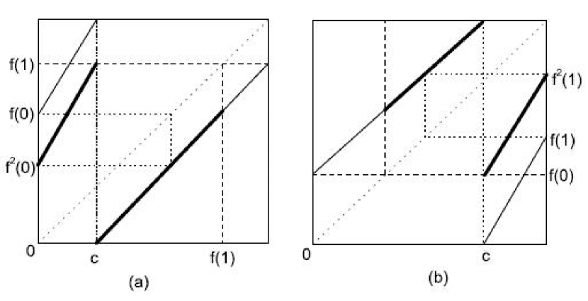
Figure 1. Trivial renormalization of a map on $[0,\ 1]$, the pictures of $g$: (a) $c\leq f(0)$,  (b) $f(1)\leq c$.

Denote $O_{f}$ and $O_{g}$ as the periodic orbit with minimal period of $f$ and $g$, and $D(f)$ and $D(g)$ as the minimal completely invariant closed set of $f$ and $g$, respectively.

If $c\leq f(a)$, by (13), we get $O_{g}=O_{f}\cap[a,\ f(b)]$, and $D(g)=D(f)\cap[a,\ f(b)]$. It follows that $D(f)=I$ is if and only if $D(g)=[a,\ f(b)]$, and $D(f)=O_{f}$ if any only if $D(g)=O_{g}$.

If $c\geq f(b)$, by (15), we obtain $O_{g}=O_{f}\cap[f(a),\ b]$, and $D(g)=D(f)\cap[f(a),\ b]$. It follows that $D(f)=I$ is if and only if $D(g)=[f(a),\ b]$, and $D(f)=O_{f}$ if any only if $D(g)=O_{g}$.

In both cases, according to Theorem B in [2], we know that $f$ is renormalizable if and only if $g$ is renormalizable. Moreover, if $f$ is renormalizable, the minimal renormalization of $f$ is periodic if and only if the minimal renormalization of $g$ is periodic. ∎

It is easy to see that a Lorenz map with $c\in(f(a),\ f(b))$ can not be trivially renormalizable, so the statement in Proposition 2 is just the the fact that an expanding Lorenz map $f$ is trivially renormalizable if and only if $c\notin(f(a),\ f(b))$.

Applying trivial renormalization (see Proposition 2, (13) and (15)) consecutively if possible, we get the following Corollary.

Corollary 1.

Let $f$ be an expanding Lorenz map with minimal period $\kappa$. If $\kappa<\infty$, then $f$ can be trivially renormalized finite times to be an expanding Lorenz map $g$ with $\kappa(g)\leq 2$.

3. Expansion of nice pair

Suppose $p$ is a periodic point with period $m$. $p$ is called a nice periodic point if $f^{m}$ is continuous on the interval between $p$ and the critical point $c$. $\{p,\ q\}$ is called a nice pair if $p<c<q$, and both $p$ and $q$ are nice periodic points. If $E$ is a proper completely invariant closed set of $f$, $e_{-}$ and $e_{+}$ are defined by (3), then $\{e_{-},\ e_{+}\}$ is a nice pair. A nice pair $\{p,\ q\}$ corresponds to a renormalization if and only if $[f^{r}(c_{+}),\ f^{\ell}(c_{-})]\subseteq[p,\ q]$, where $\ell$ and $r$ are the periods of $p$ and $q$, respectively.

Assume that $f\in\mathcal{L}_{2}$, by Lemma 1, $f$ admits a two periodic orbit $O=\{P_{L},\ P_{R}\}$, and $0<P_{L}<c<P_{R}<1$. Let $\{p,\ q\}$ be a nice pair of $f$, $\ell$ and $r$ be the period of $p$ and $q$, respectively. So $f^{\ell}$ is linear on $[p,\ c_{-}]$, and $f^{r}$ is linear on $[c_{+},\ q]$. Put

(16) $$\left\{\begin{aligned} M_{p}:&=(f^{\ell})^{\prime}(p)=(f^{\ell})^{\prime}(c_{-})=\prod_{i=0}^{\ell-1}f^{\prime}(f^{i}(c_{-})),\\ M_{q}:&=(f^{r})^{\prime}(q)=(f^{\ell})^{\prime}(c_{+})=\prod_{i=0}^{r-1}f^{\prime}(f^{i}(c_{+})).\end{aligned}\right.$$

The main purpose of this section is to prove the following expansion of nice pair for maps in $\mathcal{L}_{2}$, which is essential for us to obtain the Dichotomy (9).

Theorem 1.

Suppose $f\in\mathcal{L}_{2}$, $\{p,\ q\}$ is a nice pair of $f$, and $M_{p}$ and $M_{q}$ are defined as above. If   $[f(0),\ f(1)]\nsubseteq[P_{L},\ P_{R}]$, then

(17) $$(M_{p}-1)(M_{q}-1)>1.$$

Remark 2.

By (6) and the trichotomy claimed by Theorem B in [2] , $[f(0),\ f(1)]\nsubseteq[P_{L},\ P_{R}]$ is equivalent to $D\neq O$.

The proof of Theorem 1 is technical. Let $f\in\mathcal{L}_{2}$ such that $D\neq O$, we divide the proof into three cases: both $a\geq 1$ and $b\geq 1$, $a<1<b$ and $a>1>b$. In the first case, all of the factors in the product of $M_{p}$ and $M_{q}$ are no less than $1$, it is easier to get the lower bounds of $M_{p}$ and $M_{q}$. In fact, the expansion of a nice pair (17) can be achieved by Lemma 4, which is a direct consequence of some inequalities obtained from the action of $f$ on some intervals. The second case and the third case are similar. In order to get a lower bound for $M_{p}$ and $M_{q}$ when $a<1<b$, we introduce the first exit decomposition. Although $f$ is contractive on the left side of the critical point, we try to decompose $M_{p}$ and $M_{q}$ into parts so that each part is no less than $1$. Depending on the position of $f(0)=1-ac$, we have three cases. In each case, we can obtain lower bound of $M_{p}$ and $M_{q}$ to ensure (17). In the remain parts of this section, we introduce the first exit decomposition firstly, then we prove some technical Lemmas based on the detailed dynamics of $f$, and prove Theorem 1 finally.

3.1. First exit decomposition

Let $A$ be a given set, $O(x)=\{f^{j}(x);j\geq 0\}$ be the orbit with initial $x$. If $O(x)$ visits $A$, denote

$$n_{A}(x)=\min\{k:f^{k-1}(x)\in A,\ f^{k}(x)\notin A\}$$

as the first exit time of $O(x)$ from $A$, and the $s$th $(s\geq 1)$ exit time $n_{s}(x)$ from $A$ are defined inductively by

$$n_{1}(x):=n_{A}(x),\ \ n_{s}(x):=\min\{k>n_{s-1}:f^{k-1}(x)\in A,\ f^{k}(x)\notin A\}.$$

If $O(x)$ does not visit $A$, $n(x)=\infty$.

Denote $x_{s}:=f^{n_{s}}(x),\ \ s=1,2,\ldots$. Put

$$M_{A}(x)=\prod_{j=0}^{n_{A}(x)-1}f^{\prime}(f^{j}(x)).$$

Using above notations, the following first exit decomposition is trivial.

Lemma 2.

$x\in I$, and $n_{s}(x)\leq n<n_{s+1}(x)$,

(18) $$(f^{n})^{\prime}(x)=\prod_{j=0}^{n-1}f^{\prime}(f^{j}(x))=M_{A}(x)M_{A}(x_{1})\cdots M_{A}(x_{s-1})W(x_{s}),$$

where

$$W(x_{s})=f^{\prime}(x_{s})f^{\prime}(f(x_{s}))\cdots f^{\prime}(f^{n-1}(x)),$$

and $W(x)=1$ if and only if $x_{s}=f^{n}(x)$.

3.2. Technical Lemmas

Suppose $f:=f_{a,b,c}\in\mathcal{L}_{2}$. Denote the $2$-periodic points are $P_{L}$ and $P_{R}$, $0<P_{L}<c<P_{R}<1$, and $c_{*}$ and $c^{*}$ are the preimages of $c$, $0<c_{*}<P_{L}<c<P_{R}<c^{*}<1$. By direct calculations, we get

(19) $$P_{L}=\frac{b(c-(1-ac))}{ab-1},\ \ \ \ \ P_{R}=\frac{abc-(1-ac)}{ab-1}$$

$$c_{*}=\frac{c-(1-ac)}{a},\ \ \ \ \ \ \ \ \ \ \ \ \ \ \ \ \ \ \ c^{*}=\frac{c+bc}{b}.$$

Observe that $f^{2}$ is linear (with slope $ab=f^{2}(P_{L})>1$) on $[c_{*},\ P_{L}]$, and $f^{2}(P_{L})=P_{L}$. Track the preimages of $c_{*}$ on $[c_{*},\ P_{L}]$, one can get an increasing sequence $\{c_{n}\}\subset[c_{*},P_{L}]$,

(20) $$c_{0}:=c_{*},\ \ f^{2}(c_{1})=c_{0},\ \cdots,\ f^{2}(c_{n})=c_{n-1},\ \cdots$$

and $c_{n}\uparrow P_{L}$. $(c_{*},P_{L})=\bigcup_{k\geq 1}(c_{k-1},\ c_{k}]$. Similarly, there exists a decreasing sequence $\{c_{n}^{\prime}\}$ approaches to $P_{R}$ so that

(21) $$c_{0}^{\prime}:=c^{*},\ \ f^{2}(c_{1}^{\prime})=c_{0}^{\prime},\ \cdots,\ f^{2}(c_{n}^{\prime})=c_{n-1}^{\prime},\ \cdots.$$

Lemma 3.

Let $\{c_{n}\}$ and $\{c_{n}^{\prime}\}$ are defined as (20) and (21), we have

(22) $$|(c_{n-1},\ c_{n})|\leq|(c_{n},\ c)|,$$

(23) $$|(c^{\prime}_{n},\ c_{n-1})|\leq|(c,\ c^{\prime}_{n})|.$$

Proof.

At first, we prove (22). Using (19),

$$|(c_{*},\ P_{L})|=\frac{c-(1-ac)}{a(ab-1)},\ \ |(P_{L},\ c)|=\frac{a(b(1-c)-c)}{c-(1-ac)}|(c_{*},\ P_{L})|.$$

Since $f^{2k}$ maps $(c_{k},\ P_{L})$ homeomorphically to $(c_{*},\ P_{L})$,

$$|(c_{n},\ P_{L})|=\frac{1}{a^{n}b^{n}}|(c_{*},\ P_{L})|,\ \ \ \ \ \ |(c_{n-1},\ P_{L})|=\frac{1}{a^{n-1}b^{n-1}}|(c_{*},\ P_{L})|.$$

It follows that

$$|(c_{n-1},\ c_{n})|=|(c_{n-1},\ P_{L})|-|(c_{n},\ P_{L})|=(\frac{1}{a^{n-1}b^{n-1}}-\frac{1}{a^{n}b^{n}})|(c_{*},\ P_{L})|,$$

and

$$|(c_{n},\ c)|=|(c_{n},\ P_{L})|+|(P_{L},\ c)|=(\frac{1}{a^{n}b^{n}}+\frac{a(b(1-c)-c)}{c-(1-ac)})|(c_{*},\ P_{L})|.$$

Hence, (22) is equivalent to

(24) $$\frac{2}{ab}+(ab)^{n-1}\frac{a(b(1-c)-c)}{c-(1-ac)}\geq 1.$$

Remember that $f$ satisfies the additional condition (7), i.e., $0<f(0)=1-ac<c<b(1-c)=f(1)<1$, $\frac{a(b(1-c)-c)}{c-(1-ac)}$ is always positive.

Since $ab>1$, it is enough to prove (24) with $n=1$, i.e.,

(25) $$F(b):=\frac{2}{ab}+\frac{a(b(1-c)-c)}{c-(1-ac)}\geq 1.$$

If $ab\leq 2$, then $F(b)\geq\frac{2}{ab}\geq 1$. For the case $ab>2$, $a$ is fixed,

$$F^{\prime}(b)=-\frac{2}{ab^{2}}+\frac{a(1-c)}{c-(1-ac)}=\frac{a^{2}b^{2}(1-c)-2(c-(1-ac))}{ab^{2}(c-(1-ac))}.$$

Using $ab>2$ and $f(1)=b(1-c)>c$,

$$a^{2}b^{2}(1-c)-2(c-(1-ac))>a^{2}bc-2c+2-2ac>ac(ab-2)+2(1-c)>0.$$

So $F^{\prime}(b)>0$ when $ab>2$. It follows that $F(b)>F(\frac{2}{a})=1$. (25) holds.

For the second inequality, by similar calculations, one can see that (23) is equivalent to

(26) $$\frac{2}{ab}+(ab)^{n-1}\frac{b(c-(1-ac))}{b(1-c)-c}\geq 1.$$

We shall prove (26) with $n=1$, i.e.,

(27) $$G(a):=\frac{2}{ab}+\frac{b(c-(1-ac))}{b(1-c)-c}\geq 1.$$

If $ab\leq 2$, then $G(a)\geq\frac{2}{ab}\geq 1$. When $ab>2$,

$$G^{\prime}(a)=-\frac{2}{a^{2}b}+\frac{bc}{b(1-c)-c}=\frac{a^{2}b^{2}c-2(b(1-c)-c)}{a^{2}b(b(1-c)-c)}.$$

Using $ab>2$ and $f(0)=1-ac<c$, one obtains

$$a^{2}b^{2}c-2(b(1-c)-c)>2abc-2b(1-c)+2c>2b(c-(1-ac))+2c>0.$$

So $G^{\prime}(a)>0$ when $ab>2$. It follows that $G(a)>G(\frac{2}{b})=1$. (27) holds.

∎

Lemma 4.

Let $\{c_{n}\}$ and $\{c_{n}^{\prime}\}$ be defined as (20) and (21).

1. Suppose $f(0)\in(c_{k-1},\ c_{k}]$, we have

   $$aba^{k+1}b^{k}>1+a^{k+1}b^{k}\ \ \ \ \ \ \ and\ \ \ \ \ \ \ a^{k+1}b^{k}>1.$$

2. Suppose $f(1)\in[c_{k}^{\prime},\ c_{k-1}^{\prime})$, we have

   $$aba^{k}b^{k+1}>1+a^{k}b^{k+1}\ \ \ \ \ \ \ and\ \ \ \ \ \ \ a^{k}b^{k+1}>1.$$

Proof.

It is necessary to prove (1), (2) can be proved similarly.

Consider the interval $(c_{k},\ \ P_{L})$, since $f(0)\in(c_{k-1},\ c_{k}]$, we have

$$\begin{CD}(c_{k},P_{L})@>{f^{2k}}>{(ab)^{k}}>(c_{*},P_{L})@>{f}>{a}>(c,P_{R})@>{f^{2}}>{ab}>(f(0),P_{R})\supset(c_{k},P_{L})\cup(c,P_{R}).\end{CD}$$

So we have

$$f^{2k+3}((c_{k},P_{L}))\supset(c_{k},P_{L})\cup(c,P_{R})=f^{2k+1}((c_{k},P_{L}))\cup(c,P_{R}).$$

It follows that

$$a^{k+2}b^{k+1}|(c_{k},\ \ P_{L})|>|(c_{k},\ P_{L})|+|(c,\ P_{R})|.$$

Notice that $|(c,\ P_{R})|=a^{k+1}b^{k}|(c_{k},\ P_{L})|$, we obtain $a^{k+2}b^{k+1}>1+a^{k+1}b^{k}$.

Consider the interval $(c_{k-1},\ \ c_{k})$, we obtain

$$\begin{CD}(c_{k-1},\ \ c_{k})@>{f^{2(k-1)}}>{(ab)^{k-1}}>(c_{*},\ c_{1})@>{f^{2}}>{ab}>(0,\ c_{*})@>{f}>{a}>(f(0),\ c).\end{CD}$$

Similarly, it follows

$$a^{k+1}b^{k}|(c_{k-1},\ \ c_{k})|=|(f(0),\ c)|.$$

By Lemma 3 and the condition that $f(0)\in(c_{k-1},\ c_{k}]$,

$$a^{k+1}b^{k}=\frac{|(f(0),\ \ c)|}{|(c_{k-1},\ \ c_{k})|}>\frac{|(c_{k},\ c)|}{|(c_{k-1},\ c_{k})|}\geq 1.$$

∎

Lemma 5.

Suppose $a<1<b$, $A=[0,\ c_{*}]$,

$$M(x):=M_{A}(x)=\prod_{i=0}^{n_{A}(x)-1}f^{\prime}(f^{i}(x)),$$

where $n_{A}(x)$ is the first exit time of the orbit $O(x)$ from $A$. If $f(0)\in(c_{*},\ c)$, then

(28) $$M(x):=M_{A}(x)>1,\ \ \ \ \ \forall\ x\geq f(0).$$

Similarly, suppose $a>1>b$, $B=[c^{*},\ 1]$, $M_{B}(x)=\prod_{i=0}^{n_{B}(x)-1}f^{\prime}(f^{i}(x))$, where $n_{B}(x)$ is the first exit time of the orbit $O(x)$ from $B$. If $f(1)\in(c,\ c^{*})$, then

(29) $$M_{B}(x)>1,\ \ \ \ \ \forall\ x\leq f(1).$$

Proof.

We only prove the Lemma for case $a<1<b$, the proof can adapt to the case $a>1>b$ easily.

Since $f(x)>c$ for all $x\in(c_{*},\ c)$ and $ab>1$, we know that $M(x)=\infty$ when $n_{A}(x)=\infty$. In what follows, we show that $M(x)>1$ for $x\in I$ with $n_{A}(x)<\infty$.

The main reason for us to consider the first exit decomposition with respect to $A=[0,\ c_{*}]$ is that $f$ maps $(c_{*},\ c)$ homeomorphically to $(c,\ 1)$, which implies that any orbit with initial position $x\notin A$ can not stay on the left of $c$ two consecutive times before it visits $A$. This fact is useful for us to obtain lower bound of $M_{A}(x)$.

When $f(0)>c_{*}$, each orbit of $f$ can stay on the left of $c$ at most two consecutive times. To check (28), we consider three cases:

If $x\geq c_{+}$, the product $M(x)$ begin with $b$ and end with only one $a$, and it can not have two consecutive $a$. So $M(x)>1$ because $ab>1$.

If $x\in(P_{L},\ c_{-}]$, then $f(x)\in(P_{R},\ 1]$. There is a nonnegative integer $m$ such that $f^{2m}(f(x))\geq c^{*}$. So $f^{2m+2}(x)\geq c$ and $M(f^{2m+2}(x))>1$. It follows

$$M(x)=(ab)^{m+1}M(f^{2m+2}(x))>1.$$

If $f(0)\in(c_{*},\ P_{L})$, there exists positive integer $k$ so that $f(0)\in(c_{k-1},\ P_{L})$. For $x\in(f(0),\ P_{L})$, one can see $M(x)=(ab)^{m}a^{k+1}b^{k}$ for some $m\geq 0$. By Lemma 4,

$$M(x)\geq a^{k+1}b^{k}>1.$$

∎

Let $i=\min\{k:f^{k}(0)>c\}$ be the least integer so that $f^{i}(0)>c$. Each orbit of $f$ can stay consecutively on the left of $c$ at most $i$ times. $f(0)\leq c_{*}$ implies $i\geq 3$.

Let $j=\min\{k:f^{k}(1)<c\}$ be the least integer so that $f^{i}(1)<c$. $f(1)\geq c^{*}$ implies $j\geq 3$.

Lemma 6.

Let $i$ and $j$ be defined as above, we have

(30) $$ba^{i-1}>1+a+\cdots+a^{i-2},$$

(31) $$ab^{j-1}>1+b+\cdots+b^{j-2}.$$

Proof.

Since $i$ is the least positive integer such that $f^{i-1}(0)<c<f^{i}(0)$, by direct calculation,

$$f(0)=1-ac,f^{2}(0)=(1-ac)(1+a),\ \ldots,f^{i-1}(0)=(1-ac)(1+a+\cdots+a^{i-2})<c.$$

It follows

$$c>\frac{1+a+\cdots+a^{i-2}}{1+a+\cdots+a^{i-1}}.$$

On the other hand, by assumption (7), $c<f(1)=b(1-c)$ implies $c<\frac{b}{1+b}$. We get

$$\frac{1+a+\cdots+a^{i-2}}{1+a+\cdots+a^{i-1}}<\frac{b}{1+b},$$

which is equivalent to (30).

(31) can be proved by similar calculations. ∎

Remember that $c_{1}$ and $c_{1}^{\prime}$ are defined by (20) and (21).

Lemma 7.

Let $i$ and $j$ be defined as above, we have

(32) $$ba^{i}<1\ \ \ \ \ \ implies\ \ \ \ \ \ f^{i-1}(0)\in(c_{1},\ c),$$

(33) $$ab^{j}<1\ \ \ \ \ \ implies\ \ \ \ \ \ f^{j-1}(1)\in(c,\ c_{1}^{\prime}).$$

Proof.

We only show (32). By the definition of $i$,

$$0<f(0)<f^{2}(0)<\cdots<f^{i-1}(0)<c<f^{i}(0).$$

Since $f^{i-1}$ maps $(0,\ f(0))$ to $(f^{i-1}(0),\ f^{i}(0))\ni c$ homeomorphically, there exists $y\in(0,\ f(0))$ so that $f^{i-1}(y)=c$.

Observe that

$$\begin{CD}(c_{*},\ \ c_{1})@>{f^{2}}>{ab}>(0,\ c_{*}),\end{CD}$$

there exists $z\in(c_{*},\ \ c_{1})$ such that $f^{2}(z)=y$.

Consider the interval $(c_{*},\ \ z)$, we have

$$\begin{CD}(c_{*},\ \ z)@>{f^{2}}>{ab}>(0,\ y)@>{f^{i-1}}>{a^{i-1}}>(f^{i-1}(0),\ c).\end{CD}$$

It follows that

$$ba^{i}|(c_{*},\ \ z)|=|(f^{i-1}(0),\ \ c)|.$$

If $f^{i-1}(0)<c_{1}$, by Lemma 3,

$$ba^{i}=\frac{|(f^{i-1}(0),\ \ c)|}{|(c_{*},\ \ z)|}>\frac{|(c_{1},\ c)|}{|(c_{*},\ c_{1})|}\geq 1.$$

We obtain a contradiction. Hence, (32) is true. ∎

Lemma 8.

Suppose $a<1<b$, $A=[0,\ c_{*}]$, $M(x):=M_{A}(x)$ is defined as in (28). If $f(0)<c_{*}$, then

(34) $$M(x):=M_{A}(x)>1,\ \ \ \ \ \forall x\geq c_{1}.$$

Similarly, Suppose $a>1>b$, $B=[c^{*},\ 1]$, $M_{B}(x)$ is defined as in (29). If $f(1)>c^{*}$, then

(35) $$M_{B}(x)>1,\ \ \ \ \ \forall x\leq c_{1}^{\prime}.$$

Proof.

Let $i$ be defined as above. If $x\in(c_{1},\ c_{2}]$, then $M(x)=ababa^{m}$ for some $0<m\leq i-1$. Since $a<1<b$, we have $M(x)\geq ababa^{i-1}\geq(ba^{2})(ba^{i-1})\geq 1$. In fact, Lemma 7, together with $i\geq 3$, implies that both $ba^{i-1}$ and $ba^{2}$ are no less than $1$. The remain cases can be shown by similar arguments in the proof of Lemma 5.

∎

3.3. Proof of Theorem 1

Now we present the proof of Theorem 1.

Let $f\in\mathcal{L}_{2}$, $p$ is an $\ell$-periodic point and $q$ is a $r$-periodic point of $f$, $\{p,\ q\}$ is a nice pair of $f$, and

$$M_{p}=(f^{\ell})^{\prime}(c_{-})=\prod_{i=0}^{\ell-1}f^{\prime}(f^{i}(c_{-})),\ \ \ \ \ M_{q}=(f^{r})^{\prime}(c_{+})=\prod_{i=0}^{r-1}f^{\prime}(f^{i}(c_{+})).$$

Each factor in $M_{p}$ and $M_{q}$ is either $a$ or $b$ because $f$ is piecewise linear.

Our aim is to show that

$$(M_{p}-1)(M_{q}-1)>1$$

for each nice pair $\{p,\ q\}$ provided $[f(0),\ f(1)]\nsubseteq[P_{L},\ P_{R}]$. Remember that $P_{L}$, $P_{R}$, $c_{*}$ and $c^{*}$ are all calculated in (19).

The proof can be divided into three cases: both $a\geq 1$ and $b\geq 1$, $a<1<b$, and $a>1>b$.

Case A: $a\geq 1$ and $b\geq 1$.

Since $[f(0),\ f(1)]\nsubseteq[P_{L},\ P_{R}]$, we have $f(0)<P_{L}$ or $f(1)>P_{R}$. Without loss of generality, we assume $f(1)>P_{R}$. It follows either $f(1)\in(P_{R},c^{*})$ or $f(1)\geq c^{*}$.

If $f(1)\in(P_{R},c^{*})$, there exists $k$ so that $f(1)\in[c_{k}^{\prime},\ c_{k-1}^{\prime})$, by Lemma 4, we have $aba^{k}b^{k+1}>1+a^{k}b^{k+1}$. $p$ is a nice $\ell$-periodic point indicates $\ell\geq 2k+3$. In fact, in this case, when $m<2k+2$, the interval $(f^{m}(p),\ f^{m}(c_{-}))$ does not contain $c_{*}$ and $c^{*}$, so $N((f^{2k+2}(p),\ f^{2k+2}(c_{-})))\geq 1$. Since $a\geq 1$ and $b\geq 1$, $M_{p}=aba^{k}b^{k+1}\prod_{i=2k+3}^{\ell-1}f^{\prime}(f^{i}(c_{-}))\geq aba^{k}b^{k+1}$ and $M_{q}=ab\prod_{i=2}^{r-1}f^{\prime}(f^{i}(c_{+}))\geq ab$. Hence,

$$(M_{p}-1)(M_{q}-1)\geq(aba^{k}b^{k+1}-1)(ab-1)>a^{k}b^{k+1}(ab-1)>1.$$

If $f(1)\geq c^{*}$, by similar arguments as above, we get $M_{p}\geq ab^{2}>1+b$ by Lemma 6. Hence, using $M_{q}\geq ab$, we obtain

$$(M_{p}-1)(M_{q}-1)\geq(ab^{2}-1)(ab-1)>b(ab-1)>1.$$

Therefore, the expansion of nice pair (17) is proved when both $a$ and $b$ are no less than $1$.

Case B: $a<1<b$.

In this case, $f$ is contractive on the left side of $c$. We consider the first exit decomposition of $M_{p}$ and $M_{q}$ with respect to $A=[0,\ c_{*}]$. Since $f$ maps $(c_{*},\ c)$ homeomorphically to $(c,\ 1)$, any orbit with initial position $x\notin A$ can not stay on the left of $c$ two consecutive times before it visits $A$.

Suppose $O_{r}(c_{+}):=\{c_{+},\ f(c_{+}),\ \ldots,f^{r-1}(c_{+})\}$ exits $A=[0,\ c_{*}]$ exact $s$ ($s\geq 1$) times. Put $x_{j}:=f^{n_{j}}(c_{+})$, where $n_{j}$ is the $j$th exit time for the finite orbit $O_{r}(c_{+})$ with respect to $A$. According to the first exit decomposition (18),

$$M_{q}=(f^{r})^{\prime}(c_{+})=\prod_{k=0}^{r-1}f^{\prime}(f^{k}(c_{+}))=M(c_{+})M(x_{1})\cdots M(x_{s-1})W(x_{s}),$$

where $W(x_{s})=f^{\prime}(x_{s})f^{\prime}(f(x_{s}))\cdots f^{\prime}(f^{r-1}(c_{+}))$. $W(x_{s})\geq 1$ because it can not contain two consecutive $a$, the last factor is $b$, and $ab>1$.

Similarly, suppose $O_{\ell}(c_{-})$ exits $A$ exact $t$ times. Denote $y_{j}:=f^{n_{j}}(c_{-})$, one gets

$$M_{p}=(f^{\ell})^{\prime}(c_{-})=\prod_{k=0}^{\ell-1}f^{\prime}(f^{k}(c_{-}))=M(c_{-})M(y_{1})\cdots M(y_{t-1})W(y_{t}),$$

and $W(y_{t})=f^{\prime}(y_{t})f^{\prime}(f(y_{t}))\cdots f^{\ell-1}(c_{-})\geq 1$.

Depending on the position of $f(0)$, we distinguish three subcases: $P_{L}\leq f(0)<c$, $c_{*}<f(0)<P_{L}$ and $f(0)\leq c_{*}$. We shall show that the expansion of nice pair (17) holds in each subcase.

(i) Subcase $P_{L}<f(0)<c$.

Since $f(x)>f(0)$ for $x\in A$, by Lemma 5 we know that $M(x_{j})\geq 1$, $j=1,\cdots,s-1$, and $M(y_{j})\geq 1$, $j=1,\cdots,t-1$. It follows that $M_{q}\geq M(c_{+})=ab$ and $M_{p}\geq M(c_{-})$. Since $[f(0),\ f(1)]$ does not contained in $[P_{L},\ P_{R}]$, we get $f(1)>P_{R}$. Depend on the position of $f(1)$, we consider two cases: $f(1)\in(P_{R},\ c^{*})$ and $f(1)\geq c^{*}$.

If $f(1)\in(P_{R},\ c^{*})$, then there exists positive integer $k$ so that $f(1)\in[c_{k}^{\prime},\ c_{k-1}^{\prime}]$, by Lemma 4, $M(c_{-})\geq aba^{k}b^{k+1}$. We obtain

$$(M_{p}-1)(M_{q}-1)\geq(aba^{k}b^{k+1}-1)(ab-1)>a^{k}b^{k+1}(ab-1)>1.$$

If $f(1)\geq c^{*}$, then $f^{2}(1)\geq c$, which implies that $M(f^{2}(1))\geq 1$ because the product $M(f^{2}(1))$ begin with $b$ and it admits no consecutive $a$. We obtain $M_{p}\geq M(c_{-})\geq abbM(f^{2}(1))\geq ab^{2}$. By Lemma 6, $ab^{2}>1+b$. As a result,

$$(M_{p}-1)(M_{q}-1)\geq(ab^{2}-1)(ab-1)>b(ab-1)>1.$$

(ii) Subcase $c_{*}<f(0)<P_{L}$.

In this case, there exist $k\geq 1$ so that $f(0)\in(c_{k-1},\ c_{k}]$. Since $f(x)>f(0)$ for each $x\in A$, by Lemma 5, we know that $M(x_{j})\geq 1$ for $j=1,2,\ldots,s-1$, and $M(y_{j})\geq 1$ for $j=1,2,\ldots,t-1$. We have

$$M_{q}=M(c_{+})M(x_{1})\cdots M(x_{s-1})W(x_{s})\geq M(c_{+})M(x_{1})=aba^{k+1}b^{k}.$$

$$M_{p}\geq M(c_{-})=abM(f(1))\geq ab.$$

Using Lemma 4, we conclude that

$$(M_{p}-1)(M_{q}-1)\geq(aba^{k+1}b^{k}-1)(ab-1)>a^{k+1}b^{k}(ab-1)>1.$$

(iii) Subcase $f(0)\leq c_{*}$.

Let $i$ be the minimal positive integer so that $f^{i}(0)>c$. Each orbit can stay on the left of $c$ at most $i$ consecutive times. At first, we conclude that

(36) $$M(x)\geq ba^{i}\ \ \ \ \ \ \ \ \ \ x>c_{*}.$$

In fact, one can write $M(x)=aUba^{m}$, where $m\leq i-1$, and $U\geq 1$ because $U$ begin with $b$ and it admits no consecutive $a$. So we have $M(x)\geq aba^{i-1}=ba^{i}$ because and $a<1$.

In what follows, we shall prove

(37) $$M_{q}\geq ba^{i-1},\ \ \ \ \ \ \ M_{p}\geq ba.$$

Claim 1: $M_{q}\geq ba^{i-1}$.

Claim 1 will be proved in two separated cases: $ba^{i}\geq 1$ and $ba^{i}<1$.

Suppose $ba^{i}\geq 1$. By Lemma 2, Lemma 5 and (36),

$$M_{q}=\prod_{m=0}^{r-1}f^{\prime}(f^{m}(c_{+}))=M(c_{+})M(x_{1})\cdots M(x_{s-1})W(x_{s})\geq M(c_{+})=ba^{i-1}.$$

Now we suppose $ba^{i}<1$. By Lemma 6, we know that $ba^{i-1}>1+a+\cdots+a^{i-2}>1$. By Lemma 2,

$$M_{q}=\prod_{m=0}^{r-1}f^{\prime}(f^{m}(c_{+}))=M(c_{+})M(x_{1})\cdots M(x_{s-1})W(x_{s}),$$

where $E=f^{\prime}(x_{s})f^{\prime}(f(x_{s}))\cdots f^{\prime}(f^{r-1}(c_{+}))\geq 1$.

In what follows we show that

$$M=M(x_{1})M(x_{2})\cdots M(x_{s-1})\geq 1,$$

which implies our Claim $M_{q}\geq M(c_{+})=ba^{i-1}$.

By Lemma 8, $M(x_{j})\geq 1$ for all $x_{j}>c_{1}$. So $M\geq 1$ if there is no $x_{j}$ is smaller than $c_{1}$.

Suppose there are some $j$ so that $M(x_{j})<1$. We denote them as $j_{1}<j_{2}<\cdots$. According to Lemma 7, $ba^{i}<1$ implies $c_{1}<f^{i-1}(0)<c$. Using Lemma 8 we get $M(x_{1})>1$. As a result, we have $j_{1}>1$. By Lemma 7, we know that $x_{j_{1}}\in(c_{*},\ c_{1}]$, and $M(x_{j_{1}})=ba^{i}$ because each orbit can stay on the left of $c$ at most $i$ consecutive times and $ba^{i-1}>1$.

Let $k_{1}=max\{t:x_{t}>c_{1},t<j_{1}\}$. It follows from Lemma 7 and Lemma 8 that $1\leq k_{1}<j_{1}$ and $x_{k_{1}}>c_{1}$, which, together with $ab>1$, implies $M(x_{k_{1}})\geq ababa^{m}$. Moreover, we conclude that $m<i-1$, because $m=i-1$ implies $x_{k_{1}}>c_{1}$ by Lemma 7. We obtain $M(x_{k_{1}})\geq ababa^{i-2}$. Therefore, $M(x_{k_{1}})M(x_{j_{1}})\geq ababa^{i-2}ba^{i}=(ba^{2})(ba^{i-1})(ba^{i-1})\geq 1$.

By similar arguments, one can find $j_{1}<k_{2}<j_{2}$ so that $M(x_{k_{2}})M(x_{j_{2}})\geq 1$. Repeat the above procedures several times if possible, we conclude that $M\geq 1$. Therefore, $M_{q}\geq M(c_{+})=ba^{i-1}$.

Claim 1 is true.

Claim 2: $M_{p}\geq ab.$

Since the orbit

$$O_{\ell}(c_{-})=\{c_{-},\ 1,\ f(1),\ \ldots,\ f^{\ell-1}(c_{-})\}$$

exits $A$ exact $s(\geq 0)$ times, and the first point after $j$th exit is $y_{j}$, we conclude that

(38) $$\begin{split}M_{p}=(f^{\ell})^{\prime}(c_{-})&=M(c_{-})M(y_{1})\cdots M(y_{t-1})W\\ &=abM(f(1))M(y_{1})\cdots M(y_{t-1})W\end{split}$$

where $W=f^{\prime}(y_{t})f^{\prime}(f(y_{t}))\cdots f^{\prime}(f^{\ell-1}(c_{-}))$.

Using the same arguments in the proof of Claim 1, one can show that both $M(f(1))M(y_{1})\cdots M(y_{t-1})$ and $W$ are greater than $1$. Claim 2 holds.

Using (37) and Lemma 6,

$$(M_{p}-1)(M_{q}-1)\geq(ab-1)(ba^{i-1}-1)>(ab-1)a^{i-2}>1.$$

So the expansion of nice pair (17) is proved when $a<1<b$.

Case C: $a>1>b$.

One can adapt the proof of the case $a<1<b$ to this case by using the first exit decomposition of $M_{p}$ and $M_{q}$ with respect to the set $B=[c^{*},\ 1]$. $\hfill\Box$

4. Proof of Main Theorem’

Now we are ready to prove the Main Theorem’, which, together with Proposition 1, implies our Main Theorem.

Proof.

It is proved in [3] that a piecewise linear Lorenz map that expand on average is always expanding. During the proof, we denote the piecewise linear Lorenz map $f_{a,b,c}$ by $f\in\mathcal{L}$.

Step 1. Since the renormalization of piecewise linear Lorenz map is still piecewise linear, in order to prove each renormalization of $f$ is periodic, it is necessary to show that the minimal renormalization of any renormalizable piecewise linear Lorenz map is always periodic.

If $f$ does not satisfy the additional condition $1-ac<c<b(1-c)$, by Proposition 2, there is an expanding Lorenz map $g$ with minimal period $\kappa(g)<\kappa(f)$, such that $f$ is renormalizable if and only if $g$ is renormalizable, and if $f$ is renormalizable, then minimal renormalization of $f$ is periodic if and only if the minimal renormalization of $g$ is periodic. Furthermore, since $f$ is piecewise linear with $ac+b(1-c)>1$, $g\in\mathcal{L}$.

Applying Proposition 2 several times if necessary, we can assume that $\kappa(f)\leq 2$ (see Corollary 1). It follows from Proposition 2 that $f\in\mathcal{L}$ can not be renormalized trivially if and only if either $\kappa(f)=1$ or $f\in\mathcal{L}_{2}$. Since any expanding Lorenz map with $\kappa(f)=1$ is prime, we only need to consider the case $f\in\mathcal{L}_{2}$.

Step 2. Suppose that $f\in\mathcal{L}_{2}$. Let $O=\{P_{L},\ P_{R}\}$ be the 2-periodic points of $f$, and $P_{L}<c<P_{R}$, $D=\bigcup_{n\geq 0}f^{-n}(O)$ be the minimal completely invariant closed set of $f$. We shall prove $f$ is prime if $D\neq O$ by contradiction.

Now suppose $f$ is not prime, according to Theorem A in [2], the minimal renormalization map of $f$ is $Rf$,

$$Rf(x)=\left\{\begin{array}[]{ll}f^{\ell}(x)&x\in[f^{r}(c_{+}),c)\\ f^{r}(x)&x\in(c,f^{\ell}(c_{-})],\end{array}\right.$$

where $p=\sup\{x<c:x\in D\},\ q=\inf\{x>c:x\in D\}$, and $\ell$ and $r$ are the maximal integers so that $f^{\ell}$ and $f^{r}$ is continuous on $(p,\ c)$ and $(c,\ q)$, respectively. Obviously, $\{p,\ q\}$ is a nice pair.

Put $L=(p,\ c)$, $R=(c,\ q)$, $M_{p}=(f^{\ell})^{\prime}(p)$ and $M_{q}=(f^{r})^{\prime}(q)$. Since $Rf$ is a piecewise linear Lorenz map, we have

$$|f^{\ell}(L)|=|f^{\ell}((p,\ c))| = |(p,\ f^{\ell}(c_{-}))|=M_{p}|L|\leq|L|\ +\ |R|$$

$$|f^{r}(R)|=|f^{r}((c,\ q))| = |(f^{r}(c_{+}),\ q)|=M_{q}|R|\leq|L|\ +\ |R|,$$

which implies

(40) $$(M_{p}-1)(M_{q}-1)\leq 1.$$

On the other hand, if $D\neq O$, then $[f(0),\ f(1)]\nsubseteq[P_{L},\ P_{R}]$ by (6). According to Theorem 1, we have

$$(M_{p}-1)(M_{q}-1)>1$$

because $\{p,\ q\}$ is a nice pair. We obtain a contradiction.

It follows that $f$ is prime if $D\neq O$. So we conclude that the minimal renormalization of $f$ is periodic. As a result, each renormalization of $f$ is periodic.

Step 3. Now we show that $f$ can only be renormalized finite times. If $f$ is renormalizable, then the minimal renormalization $Rf$ is a $\beta$-transformation because $Rf$ is a periodic renormalization indicates $M_{p}=M_{q}$. So $g:=Rf$ is a $\beta$-transformation with slope $M_{p}$, which can be renormalized at most finite times by (40). As a result, $f$ can be renormalized at most finite times.

∎

Acknowledgements: This work is partially supported by a grant from the Spanish Ministry (No.SB2004-0149) and grants from NSFC (Nos.60534080,70571079) in China. Ding thanks Centre de Recerca Matem$\grave{a}$tica for the hospitality and facilities.

References

- [1] L. Alsed, A. Falc, On the topological dynamics and phase-locking renormalization of Lorenz-like maps, Ann. Inst. Fourier (Grenoble) 53 (2003), no. 3, 859–883.
- [2] Y. M. Ding, Renormalization and -limit set for expanding Lorenz map, preprint, 2007.
- [3] Y. M. Ding, A. H. Fan and J. H. Yu, The acim of piecewise linear Lorenz map, preprint, 2006.
- [4] N. Dobbs. Renormalisation-induced phase transitions for unimodal maps, Comm. Math. Phys. 286 (2009), no. 1, 377–387.
- [5] L.Flatto and J. C. Lagarias, The lap-counting function for linear mod one transformations, I. Explicit formulas and renormalizability. Ergodic Theory Dynam. Systems 16 (1996), no. 3, 451–491.
- [6] L. Flatto and J. C. Lagarias, The lap-counting function for linear mod one transformations, II. the Markov chain for generalized lap numbers. Ergodic Theory Dynam. Systems 17 (1997), no. 1, 123–146.
- [7] L.Flatto and J. C. Lagarias, The lap-counting function for linear mod one transformations. III. The period of a Markov chain. Ergodic Theory Dynam. Systems 17 (1997), no. 2, 369–403.
- [8] A. O. Gelfond, A common property of number systems, Izv. Akad. Nauk SSSR. Ser. Mat. 23(1959) , 809-814.
- [9] P. Glendinning, Topological conjugation of Lorenz maps by -transformations, Math. Proc. Camb. Phil. Soc., 107 (1990), 401–413.
- [10] P. Glendinning and T. Hall, Zeros of the kneading invariant and topological entropy for Lorenz maps, Nonlinearity, 9 (1996), 999–1014.
- [11] P. Glendingning and C. Sparrow, Prime and renormalizable kneading invariants and the dynamics of expanding Lorenz maps, Physica D, 62 (1993), 22–50.
- [12] R. Labarca and C. G. Moreira, Essential Dynamics for Lorenz maps on the real line and the Lexicographical World, Annales de l’Institut Henri Poincare (C) Non Linear Analysis, (23) (2006), no. 5, 683–694.
- [13] M. I. Malkin, Rotation intervals and the dynamics of Lorenz type mappings, Selecta Mathematica Sovietica, 10 (1991), 265–275.
- [14] M. Martens and W. de Melo, Universal models for Lorenz maps, Ergodic Theory Dynam. Systems, 21 (2001), 833–860.
- [15] J. Milnor and W. Thurston, On iterated maps of the interval, in Dynamical systems (College Park, MD, 1986-87), 465-563, in Lecture Notes in Math., 1342, Springer, Berlin, 1988.
- [16] M. R. Palmer, On the classification of measure preserving transformations of Lebesgue spaces, Ph. D. thesis, University of Warwick , 1979.
- [17] W. Parry, On the -expansions of real numbers, Acta Math. Acad. Sci. Hungar., 11 (1960), 401–416.
- [18] W. Parry, Representations for real numbers, Acta Math. Acad. Sci. Hungar., 15 (1964), 95–105.
- [19] W. Parry, Symbolic dynamics and transformations of the unit interval, Trans. Amer. Math. Soc., 122 (1966), 368–378.
- [20] W. Parry, The Lorenz attractor and a related population model, Ergodic theory (Proc. Conf., Math. Forschungsinst., Oberwolfach, 1978), pp. 169–187, in Lecture Notes in Math., 729, Springer, Berlin, 1979.
- [21] A. Rnyi, Representations for real numbers and their ergodic properties, Acta Math. Acad. Sci. Hungar, 8 (1957), 477-493.