Neutrino oscillations in magnetically driven supernova explosions

Abstract:

We investigate neutrino oscillations from core-collapse supernovae that produce magnetohydrodynamic (MHD) explosions. By calculating numerically the flavor conversion of neutrinos in the highly non-spherical envelope, we study how the explosion anisotropy has impacts on the emergent neutrino spectra through the Mikheyev-Smirnov-Wolfenstein effect. In the case of the inverted mass hierarchy with a relatively large $\theta_{13}$ ($\sin^{2}2\theta_{13}\gtrsim 10^{-3}$), we show that survival probabilities of $\bar{\nu}_{e}$ and $\nu_{e}$ seen from the rotational axis of the MHD supernovae (i.e., polar direction), can be significantly different from those along the equatorial direction. The event numbers of $\bar{\nu}_{e}$ observed from the polar direction are predicted to show steepest decrease, reflecting the passage of the magneto-driven shock to the so-called high-resonance regions. Furthermore we point out that such a shock effect, depending on the original neutrino spectra, appears also for the low-resonance regions, which could lead to a noticeable decrease in the $\nu_{e}$ signals. This reflects a unique nature of the magnetic explosion featuring a very early shock-arrival to the resonance regions, which is in sharp contrast to the neutrino-driven delayed supernova models. Our results suggest that the two features in the $\bar{\nu}_{e}$ and $\nu_{e}$ signals, if visible to the Super-Kamiokande for a Galactic supernova, could mark an observational signature of the magnetically driven explosions, presumably linked to the formation of magnetars and/or long-duration gamma-ray bursts.

1 Introduction

Current estimates of Galactic core-collapse supernovae rates predict one core-collapse supernova event every $\sim 40\pm 10$ year (e.g., [1]). When a massive star ($\gtrsim 10M_{\odot}$) [2] undergoes a core-collapse supernova explosion in our Galactic center, copious numbers of neutrinos are produced, some of which may be detected on the earth. Such supernova neutrinos will carry valuable information from deep inside the core. In fact, the detection of neutrinos from SN1987A (albeit in the Large Magellanic Cloud) paved the way for Neutrino Astronomy, an alternative to conventional astronomy by electromagnetic waves [3, 4]. Even though neutrino events from SN1987A were just two dozens, they have been studied extensively and allowed us to have a confidence that the basic picture of core-collapse supernova is correct ([5, 6] see [7] for a recent review). Over the last decades, significant progress has been made in a ground-based large water Cherenkov detector as Super-Kamiokande (SK) [8] and also in a liquid scintillator detector as KamLAND [9]. If a supernova occurs in our Galactic center ($\sim 10$ kpc), about 10,000 $\bar{\nu}_{e}$ events are estimated to be detected by SK [10] (see also [11]). Those successful neutrino detections are important not only to study the supernova physics but also to unveil the nature of neutrinos itself such as the neutrino oscillation parameters the mass hierarchy, and neutrino mass [12, 13, 14, 15, 16, 17, 18](e.g., [19] for a recent review).

The neutrino flux we receive on the Earth is sensitive to the profile of the matter that the neutrinos encounter on their path. The supernova neutrinos interact with electrons when the neutrinos propagate through stellar matter via the well-known Mikheyev-Smirnov-Wolfenstein (MSW) effect [16, 20, 21, 22]. Such effects have been extensively investigated so far from various points of view, with a focus such as on the progenitor dependence of the early neutrino burst [23, 24] and on the Earth matter effects (e.g., [25, 26]).

The neutrino conversion efficiency via the MSW effect depends sharply on the density/electron fraction gradients, thus sensitive to the discontinuity produced by the passage of the supernova shock. It is rather recently that such shock effects have been focused on [14, 27, 28] (see [29] for a recent review). The time dependence of the events showing a decrease of the average energy of $\nu_{e}$ in the case of normal mass hierarchy (or $\bar{\nu}_{e}$ in the case of inverted mass hierarchy), monitors the evolution of the density profile like a tomography, thus could provide a powerful test of the mixing angle and the mass hierarchy (e.g., [17, 30, 31]). Very recently the flavor conversions driven by neutrino self-interactions are attracting great attention, because they can induce dramatic observable effects such as by the spectral split or swap (e.g., [32, 33, 34, 35] and see references therein). They are predicted to emerge as a distinct feature in their energy spectra (see [29, 36] for reviews of the rapidly growing research field and collective references therein). The resonant spin-flavor conversion has been also studied both analytically (e.g., [37, 38, 39] and references therein) and numerically (e.g., [40, 41]), which induces flavor conversions between neutrinos and antineutrinos in magnetized supernova envelopes. Those important ingredients related to the flavor conversions in the supernova environment have been studied often one by one in each study without putting all the effects together, possibly in order to highlight the new ingredient. In this sense, all the studies mentioned above should be regarded as complimentary towards the precise predictions of supernova neutrinos.

Here it should be mentioned that most of those rich phenomenology of supernova neutrinos have been based on the spherically symmetric models of core-collapse supernovae [10, 14, 23, 28]. On the other hand, there are accumulating observations indicating that core-collapse supernovae are globally aspherical commonly (e.g., [42]). Pushed by them, various mechanisms have been explored thus far by supernova modelers to understand the central engine, such as the neutrino-heating mechanism aided by convection and the standing accretion shock instability (e.g., [43, 44] and references therein), magnetohydrodynamic (MHD) mechanism relying on the extraction of the rotational energy of rapidly rotating protoneutron stars via magnetic fields (e.g., [45, 46, 47], see [19] for a recent review and collective references therein), and the acoustic mechanism relying on the acoustic energy deposition via oscillating protoneutron stars [48]. Apart from simple parametrization to mimic anisotropy and stochasticity of the shock (e.g., [49, 50]), there have been a very few studies focusing how those anisotropies obtained by the recent supernova simulations could affect the neutrino oscillations ([30, 51]). This is mainly due to the lack of multidimensional supernova models, which are generally too computationally expensive to continue the simulations till the shock waves propagate outward until they affect neutrino transformations.

Here we study the neutrino oscillations in the case of the MHD explosions of core-collapse supernovae. In this case, the highly collimated shock pushed by the strong magnetic pressure can blow up the massive stars along the rotational axis [45, 46, 47]. Such explosions are considered to precede the formations of magnetars (e.g., [45, 47, 52]), presumably linked to the so-called collapsars (e.g., [53, 54, 55]), which attract great attention recently as a central engine of long-duration gamma-ray bursts (GRBs) (e.g., [56]). By performing special relativistic simulations [47], it is recently made possible to follow the MHD explosions in a consistent manner, starting from the onset of gravitational collapse, through core-bounce, the magnetic shock-revival, till the shock-propagation to the stellar surface. Based on such models, we calculate numerically the flavor conversion in the highly non-spherical envelope through the MSW effect. For simplicity, we neglect the effects of neutrino self-interactions and the resonant spin-flavor conversion in this study. Even though far from comprehensive in this respect, we present the first discussion how the magneto-driven explosion anisotropy has impacts on the emergent neutrino spectra and the resulting event number observed by the SK for a future Galactic supernova.

The paper opens with generalities on magneto-driven explosion models and details on our numerical model (section 2). In section 3, main results are shown, in which we pay attention to the shock-effects on the so-called high-resonance in section 3.1-3.3 and on the low-resonance in section 3.4, respectively. In section 4, we give a discussion focusing on the dependence of $\theta_{13}$ and also of the original neutrino spectra on the obtained results. Summary is given in section 5 with implications of our findings.

2 Numerical method

2.1 MHD driven supernova explosion model

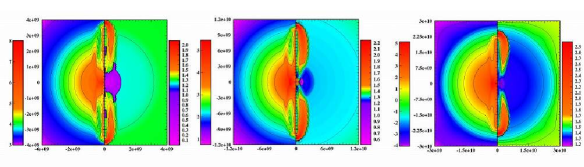
Figure 1: Snapshots showing MHD explosions of core-collapse supernovae at 0.8, 2.0 and 4.3 sec after core bounce from left to right. In each figure, contour of the logarithmic density [$\mathrm{g/cm^{3}}$] (left) and entropy per baryon [$k_{\mathrm{B}}$] (right) are shown. The unit of the horizontal and the vertical axis is in [cm]. Note that the difference of the length scale for each panel and that the outermost radius of the progenitor is $\sim 3\times 10^{10}$ [cm].

We take time-dependent density profiles from our 2.5 dimensional MHD simulations of core-collapse supernovae [47], in which a 25 M_⊙ presupernova model by Heger et al. [57] was adopted. This progenitor lacks the hydrogen and helium layer during stellar evolution, which is reconciled with observations that the progenitors associated with long-duration gamma-ray bursts are type Ib/c supernovae (e.g., [56, 58]).

For our MHD model, the strong precollapse magnetic fields of $\sim 10^{12}\mathrm{G}$ are imposed with the high angular velocity of $\sim$ 72 ${\rm rad}/{\rm s}$ with a quadratic cutoff at 100km in radius, in which the rotational energy is equal to $\sim$1% of the gravitational energy of the iron core (model B12TW1.0 in [47]). Such a combination of rapid rotation and strong magnetic field, although strong differential rotation is assumed here, have been often employed in the context of MHD supernova models [45, 47, 60].In those models, the explosion proceeds by the strong magnetic pressure amplified by the differential rotation near the surface of the protoneutron star.

One prominent feature of the MHD models is a high degree of the explosion asphericity. Figure 1 shows several snapshots featuring typical hydrodynamics of the model, from near core-bounce (0.8 s, left), during the shock-propagation (2.0 s, middle), till near the shock break-out from the star (4.3 s, right), in which time is measured from the epoch of core bounce. It can be seen that the strong shock propagates outwards with time along the rotational axis. On the other hand, the density profile hardly changes in the equatorial direction, which is a generic feature of the MHD explosions observed in recent numerical simulations [45, 47, 60].

As well known, the flavor conversion through the pure-matter MSW effect occurs in the resonance layer, where the density is

$$\rho_{\mathrm{res}}\sim 1.4\times 10^{3}\mathrm{g/cm}^{3}\left(\frac{\Delta m^{2}}{10^{-3}\mathrm{eV}^{2}}\right)\left(\frac{10\mathrm{MeV}}{E_{\nu}}\right)\left(\frac{0.5}{Y_{e}}\right)\cos 2\theta$$ (1)

where $\Delta m^{2}$ is the mass squared difference, $E_{\nu}$ is the neutrino energy, ${Y_{e}}$ is the number of electrons per baryon, and $\theta$ is the mixing angle. Since the inner supernova core is too dense to allow MSW resonance conversion, we focus on two resonance points in the outer supernova envelope. One that occurs at higher density is called the H-resonance, and the other, which occurs at lower density, is called the L-resonance. $\Delta m^{2}$ and $\theta$ correspond to $\Delta m^{2}_{13}$ and $\theta_{13}$ at the H-resonance and to $\Delta m^{2}_{12}$ and $\theta_{12}$ at the L-resonance.

Figures 3 and 3 are evolutions of the density profiles in the polar direction every 0.4 s as a function of radius. Above and below horizontal lines show approximately density of the resonance for different neutrino energies which are 5 and 60 MeV, respectively. Blue lines (left) show the range of the density of the H-resonance, and sky-blue lines (right) show that of the L-resonance. Along the polar axis, the shock wave reaches to the H-resonance, $\sim O(10^{3}$)g/cm³ at $\sim 0.5$ s, and the L-resonance, $\sim O(1)$g/cm³ at $\sim 1.2$ s. It should be noted that those timescales are very early in comparison with the ones predicted in the neutrino-driven explosion models, typically $\sim$ 5 s and $\sim$ 15 s for the H- and L- resonances, respectively (e.g., [17, 30]). This arises from the fact that the MHD explosion is triggered promptly after core bounce without the shock-stall, which is in sharp contrast to the neutrino-driven delayed explosion models ([17, 30]). The progenitor of the MHD models, possibly linked to long-duration gamma-ray bursts, is more compact due to the mass loss of hydrogen and helium envelopes during stellar evolution [59], which is also the reason for the early shock-arrival to the resonance regions.

Figure 5 shows the density profiles in the equatorial direction every 0.4 s. The profiles are almost unchanged, because the MHD shock does not reach to the outer layer for the equatorial direction. It is noted in Figures 2 and 3 that to maximize the shock effect, a sharpness of the shock along the polar direction is modified from the one in the MHD simulations, which is made to be inevitably blunt due to the employed numerical scheme using an artificial viscosity to capture shocks [47]. Green line in Figure 3 is an original density profile for 2.0 s, whose shock front is replaced with the sharp vertical surface passing through the midpoint of the blunt shock. Although our simulations are one of the state-of-the-art MHD simulations at present, which can encompass the long-term hydrodynamics starting from gravitational collapse till the shock-breakout [47], this is really a limitation of the current MHD simulations.

Snapshots labeled as (a), (b), (c), (d), (e) and (f) in Figures 3 and 3 correspond to 0.4, 0.8 and 2.8, 1.2, 2.0 and 3.2 s after bounce, respectively, which is chosen for later convenience to compute the time evolutions of the flavor conversions.

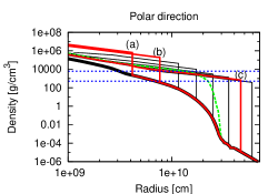
Figure 2: The density profile in the polar direction every 0.4 s as a function of radius. (a), (b) and (c) correspond to 0.4, 0.8 and 2.8 s, respectively. The horizontal blue lines show approximately density of the H-resonance for different neutrino energies which are 5 (above) and 60 MeV (below), respectively. The green line is an original density profile for 2.0 s.

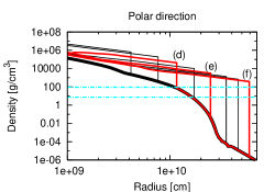
Figure 3: Same as Figure 2, but for 1.2 (d), 2.0(e), and 3.2 (f) s, respectively.

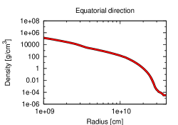
Figure 4: The density profile in equatorial direction every 0.4 s as a function of radius. The highly collimated shock does not propagate in the equatorial direction.

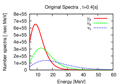
Figure 5: The original spectra at 0.4 s after core bounce taken from the Lawrence Livermore simulation (e.g., [10]). The solid line (red line), the dashed line (green) and the dotted line (blue) are $\nu_{e}$, $\bar{\nu}_{e}$ and $\nu_{x}$ spectra, respectively.

2.2 Neutrino oscillation calculations

Along the time-dependent density profiles as shown in Figures 3-5, we solve numerically the time evolution equation for the neutrino wave functions as follows,

$$\imath\frac{d}{dt}\left(\begin{array}[]{c}\nu_{e}\\ \nu_{\mu}\\ \nu_{\tau}\end{array}\right)=U\left(\begin{array}[]{ccc}0&0&0\\ 0&\Delta E_{12}&0\\ 0&0&\Delta E_{13}\end{array}\right)U^{-1}\left(\begin{array}[]{c}\nu_{e}\\ \nu_{\mu}\\ \nu_{\tau}\end{array}\right)+\left(\begin{array}[]{ccc}\sqrt{2}G_{\rm{F}}n_{e}&0&0\\ 0&0&0\\ 0&0&0\end{array}\right)\left(\begin{array}[]{c}\nu_{e}\\ \nu_{\mu}\\ \nu_{\tau}\end{array}\right),$$ (17)

where $\Delta E_{ij}=\Delta m^{2}_{ij}/2E_{\nu}$, and $\Delta m^{2}_{ij}$ are mass squared differences, $E_{\nu}$ is a neutrino energy, $G_{\rm F}$ is the Fermi constant, and $n_{e}$ is an electron number density. In the case of anti-neutrino, the sign of $\sqrt{2}\mathrm{G}_{F}n_{e}$ changes. $U$ is the Cabibbo-Kobayashi-Masukawa (CKM) matrix,

$$U=\left(\begin{array}[]{ccc}c_{12}c_{13}&s_{12}c_{13}&s_{13}e^{-i\delta}\\ -s_{12}c_{23}-c_{12}s_{23}s_{13}e^{i\delta}&c_{12}c_{23}-s_{12}s_{23}s_{13}e^{i\delta}&s_{23}c_{13}\\ s_{12}s_{23}-c_{12}c_{23}s_{13}e^{i\delta}&-c_{12}s_{23}-s_{12}c_{23}s_{13}e^{i\delta}&c_{23}c_{13}\end{array}\right),$$ (21)

where $s_{ij}=\sin{\theta}_{ij}$ and $c_{ij}=\cos{\theta}_{ij}$ ($i\neq j=1,2,3$) are the mixing angle. We set the CP violating phase, $\delta$, equal to zero in the CKM matrix for simplicity. Solving numerically the above equation, we obtain neutrino survival probabilities $P$ ($\bar{P}$) that neutrinos emitted as $\nu_{e}$ ($\bar{\nu}_{e}$) at the neutrino sphere remain $\nu_{e}$ ($\bar{\nu}_{e}$) at the surface of the star [61]. The survival probabilities are determined by an adiabaticity parameter $\gamma$,

$$\gamma = \frac{\Delta m^{2}\sin^{2}2\theta}{2E_{\nu}\cos 2\theta\left(1/n_{e}\right)(dn_{e}/dr)}.$$ (22)

$\Delta m^{2}$ and $\theta$ correspond to $\Delta m^{2}_{13}$ and $\theta_{13}$ at H-resonance, and to $\Delta m^{2}_{12}$ and $\theta_{12}$ at L-resonance, respectively. When $\gamma\gg 1$, the resonance is called “adiabatic” and the conversion between mass eigenstates does not occur. On the other hand, when $\gamma\ll 1$, the resonance is called “non-adiabatic” and the mass eigenstates are completely exchanged. If the mass hierarchy is normal, the H- and L-resonances occur only in the neutrino sector. On the other hand, if the hierarchy is inverted, the H-resonance occurs in the anti-neutrino sector, and the L-resonance occurs in the neutrino sector. The neutrino oscillation parameters are taken as $\sin^{2}2\theta_{12}$=0.84, $\sin^{2}2\theta_{23}$=1.00, $\Delta m^{2}_{12}$=8.1$\times 10^{-5}$eV² and $|\Delta m^{2}_{13}|$=2.2$\times 10^{-3}$eV² (e.g., the summary in [62] and references therein). For the unknown properties, we assume inverted mass hierarchy and $\sin^{2}2\theta_{13}$=1.0$\times$10^-3 as a fiducial value in our computations. This is because observable features in $\bar{\nu}_{e}$, most accessible channel to the SK, would imply that the neutrino mass hierarchy is inverted and that $\theta_{13}$ is large. The dependence of this parameter on the results will be discussed in Section 4.1.

The neutrino energy spectra at the surface of the star, $\phi_{\nu}^{\mathrm{SN}}(E_{\nu})$, are calculated by multiplying the survival probabilities by the original supernova neutrino spectra, $\phi^{0}_{\nu}(E_{\nu})$ [12],

$$\left(\begin{array}[]{c}\phi^{\mathrm{SN}}_{\nu_{e}}(E_{\nu})\\ \phi^{\mathrm{SN}}_{\bar{\nu_{e}}}(E_{\nu})\\ \phi^{\mathrm{SN}}_{\nu_{x}}(E_{\nu})\end{array}\right)=\left(\begin{array}[]{ccc}P(E_{\nu})&0&1-P(E_{\nu})\\ 0&\bar{P}(E_{\nu})&1-\bar{P}(E_{\nu})\\ 1-P(E_{\nu})&1-\bar{P}(E_{\nu})&2+P(E_{\nu})+\bar{P}(E_{\nu})\end{array}\right)\left(\begin{array}[]{c}\phi^{0}_{\nu_{e}}(E_{\nu})\\ \phi^{0}_{\bar{\nu_{e}}}(E_{\nu})\\ \phi^{0}_{\nu_{x}}(E_{\nu})\end{array}\right),$$ (32)

where $\phi_{\nu_{x}}\equiv 1/4(\phi_{\nu_{\mu}}+\phi_{\nu_{\tau}}+\phi_{\bar{\nu}_{\mu}}+\phi_{\bar{\nu}_{\tau}})$. To continue the simulations till the MHD shocks propagate outward until they affect neutrino transformations, the protoneutron stars are excised when the shocks comes out of the iron core. By doing so, the severe Courant-Friedrich-Levy condition in the stellar center can be relaxed, which is often taken in the long-term supernova simulation (e.g., [44, 51] and references therein). A major drawback by the excision is that the information of the neutrino spectra at the neutrino sphere is lost. Assuming that the qualitative behavior in the neutrino luminosity, such as the peaking near neutronization and the subsequent decay with time, is similar between the neutrino-heating and the MHD mechanism, we employ the results of a full-scale numerical simulation by the Lawrence Livermore group (e.g., as in [10, 31]), which predict the neutrino temperatures of $\nu_{e}$, $\bar{\nu_{e}}$ and $\nu_{x}$ to be 2.8, 4.0, and 7.0 MeV, respectively. The neutrino spectra at the neutrino sphere are approximated by Fermi-Dirac distributions and the neutrino luminosity is taken to decay exponentially with a timescale of $t_{\rm L}=3$ s (e.g., [63]). The total neutrino energy is assumed to be fixed at $2.9\times 10^{53}\mathrm{erg}$ that corresponds to the model of the Lawrence Livermore group. Figure 5 shows the original spectra at 0.4 s after core bounce. The variation of the original neutrino spectra and its effects on our results will be discussed in Section 4.2.

We calculate expected event numbers of the supernova neutrinos at a water Cherenkov detector. The positron (or electron) energy spectrum is evaluated as follows,

$$\frac{d^{2}N}{dE_{e}dt}=N_{\rm tar}\cdot\eta{(E_{e})}\cdot\frac{1}{4\pi d^{2}}\cdot\frac{d^{2}N_{\nu}}{dE_{\nu}dt}\cdot\sigma(E_{\nu})\cdot\frac{dE_{\nu}}{dE_{e}},$$ (33)

where $N$ is a detection number of neutrinos, $N_{\rm tar}$ is a target number, $\eta{(E_{e})}$ is a efficiency of the detector, $E_{e}$ is an energy of electron or positron, $d$ is a distance from the supernova, $\frac{d^{2}N_{\nu}}{dE_{\nu}dt}$ is a neutrino spectrum from the star calculated by the procedure mentioned above, and $\sigma$ is the corresponding cross section given in [61]. We consider the SK detector which is filled with 32000 ton pure water. The finite energy resolution of the detector is neglected here. The event number is obtained by integrating over the angular distribution of the events. For simplification, we take the efficiency of the detector as follows: $\eta{(E_{e})}=0$ at $E_{e}<7$ [MeV] and $\eta{(E_{e})}=1$ at $E_{e}\geq 7$ [MeV] [64]. We assume that the supernova occurs in our Galactic center ($d=$ 10 [kpc]). Albeit important [25, 26], we do not consider the Earth matter effect to highlight first the MSW effect inside the star.

3 Result

3.1 Survival probability of $\bar{\nu}_{e}$

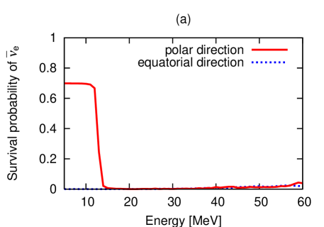
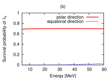
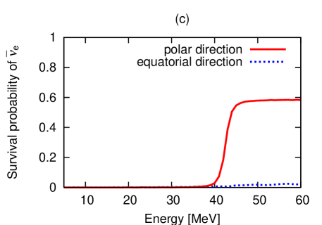
Figure 6: The survival probability of $\bar{\nu}_{e}$ in the case of (a), (b) and (c). The solid lines (red lines) and the dotted lines (blue lines) are for the polar and equatorial direction, respectively. Inverted mass hierarchy and $\sin^{2}2\theta_{13}=10^{-3}$ are assumed. The survival probability of the polar direction changes from very early stage due to the faster shock-arrival to the resonance layers than the neutrino-driven supernova models (See text for more details).

In this section, we focus on the influence of the shock wave in the H-resonance that appears in the $\bar{\nu}_{e}$ signatures in the inverted mass hierarchy. First, we calculate survival probability of $\bar{\nu}_{e}$, $\bar{P}(E_{\nu})$, in the manner described in Section 2.2.

Figure 6 is the survival probability of $\bar{\nu}_{e}$ as a function of neutrino energy in the case of (a), (b) and (c). The solid lines (red lines) and the dotted lines (blue lines) indicate that of the polar direction and the equatorial direction, respectively. The survival probability of the equatorial direction is almost 0 in all the panels. Here we focus on the survival probability of the polar direction. First, in the panel (a), the low-energy side of the survival probability becomes finite. Next, in the panel (b), the survival probability becomes finite in all the considered energy range. Finally, in the panel (c), the high-energy side of the polar direction only remains finite. The region of the finite survival probability shifts from the low-energy side to the high-energy side with time. The finite value is close to $\bar{P}\approx 0.7$ that is close to the case of the complete non-adiabatic state. It is noted that the survival probability for $\bar{\nu}_{e}$ can be given as follows (e.g., [12]),

$$\bar{P} = P_{H}\cos^{2}\theta_{12}\cos^{2}\theta_{13}+(1-P_{H})\sin^{2}\theta_{13},$$ (34)

and with the employed value of $\cos^{2}\theta_{12}=0.7$,

$$\bar{P}=0.7P_{H}\cos^{2}\theta_{13}+(1-P_{H})\sin^{2}\theta_{13},$$ (35)

where $P_{H}$ is the survival probability at the H-resonance. With the shock at the H-resonance, $P_{H}$ is close to unity, which makes $\bar{P}$ close to 0.7.

The behaviors in Figure 6 can be understood by comparing the resonance point with the shock position. When the shock front reaches the region of H-resonance (see the region enclosed by the blue lines in Figure 3), the steep decline of the density at the shock front changes the resonance into non-adiabatic following Eq. (22). As a result, the survival probability starts to become finite. As the shock propagate from the high density region to low energy region, the survival probability becomes finite from low-energy side to high-energy side, since the density at the resonance point, $\rho_{\mathrm{res}}$, is proportional to $E_{\nu}^{-1}$ (see Eq. (1)). In the equatorial direction, on the other hand, the survival probability does not change (blue dotted lines of Figure 6). This is simply because the density near the resonance along the equatorial plane hardly changes as already shown in Figure 5.

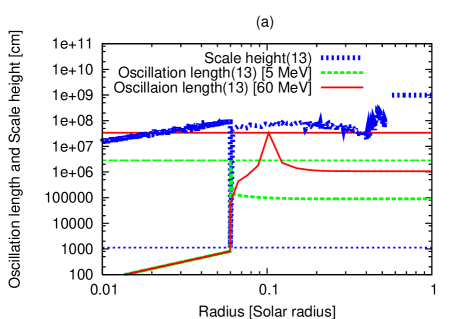
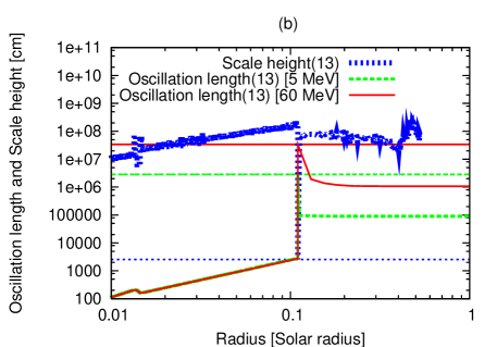
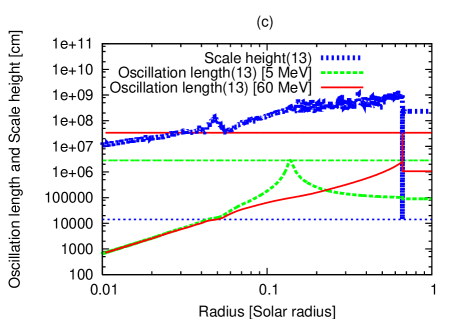
Figure 7: The dotted blue lines represent the scale height (e.g., Eq.(3.3)). The dashed green lines and the solid red lines are the oscillation length (Eq. (3.2)) of anti-neutrinos for 5 MeV and 60 MeV, respectively. Each horizontal lines are the maximum of oscillation length and the minimum values of scale height. It is noted that the label of (13) indicates that the value depends sensitively on $\theta_{13}$ and $\Delta m^{2}_{13}$.

The adiabaticity of the conversion can be evaluated by comparing the oscillation length, $L_{\mathrm{osc}}$, with the scale height of electron number density, $\delta r$ as follows,

$$\gamma = \frac{\delta r}{L_{\mathrm{osc}}}\gg 1\Longleftrightarrow\delta r\gg L_{\mathrm{osc}},$$ (36)

$$L_{\mathrm{osc}} \equiv \frac{2E_{\nu}}{\Delta m^{2}}\left[\left(\frac{2\sqrt{2}G_{F}E_{\nu}n_{e}}{\Delta m^{2}}-\cos 2\theta\right)^{2}+\sin^{2}2\theta\right]^{-\frac{1}{2}},$$ (37)

$$\delta r \equiv \frac{\sin 2\theta}{\cos 2\theta}\frac{n_{e}}{|dn_{e}/dr|},$$ (38)

When the scale height is shorter than the oscillation length, the resonance is non-adiabatic. Three panels in Figure 7 show the scale height and the oscillation length of neutrinos as a function of radius. These panels correspond to the case of (a), (b) and (c) from top to bottom. The dashed lines (green lines) and the solid lines (red lines) are the oscillation length of anti-neutrinos which energy are 5 MeV and 60 MeV, respectively. Dotted lines (blue lines) are the scale height. Most steepest decline of the scale height shown in each panel coincides with the position of the shock front. Each horizontal line indicates the maximum value of the oscillation length and the minimum value of the scale height.

In Figure 7(a), the scale height is shown to be shorter than the oscillation length of 5 MeV at the shock front at $\sim 0.06R_{\odot}$ with $R_{\odot}$ being the solar radius (compare the minimum of the blue line with the maximum of the green line, which is shown by the horizontal green line). Therefore, the H-resonance of 5 MeV becomes non-adiabatic (the survival probability $\sim$ 0.7). On the other hand, the scale height is larger, albeit slightly, than the oscillation length of 60 MeV, making the resonance adiabatic (the survival probability $\sim$ 0). In Figure 7(b), so the scale height is smaller than the oscillation length of 5 MeV and 60 MeV at the shock front ($\sim 0.1R_{\odot}$), the H-resonance for almost all the neutrino energies become non-adiabatic, making the survival probability close to be 0.7. Figure 7(c) is a direct opposition as for the resonance conditions to the case of (a). The oscillation length for the high-energy neutrinos is longer than for the low-energy neutrinos (Eq. (3.2)). This is the reason of the slight increase in the survival probability for the high-energy side seen in the equatorial direction (Figure 6).

3.2 Neutrino spectra of $\bar{\nu}_{e}$

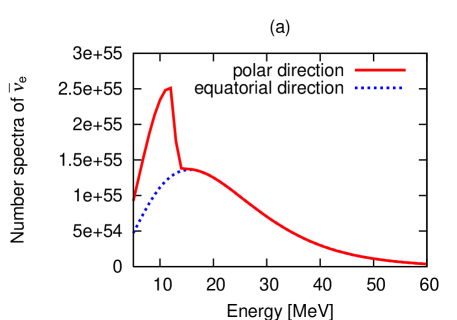
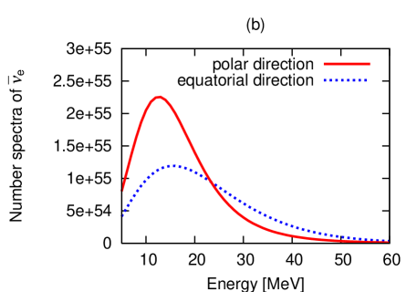
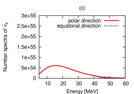
Figure 8: $\bar{\nu}_{e}$ spectra at the surface of the star in the case of (a), (b) and (c) from top to bottom. We assume the inverted mass hierarchy and $\sin^{2}2\theta_{13}=10^{-3}$. The solid lines (red lines) and the dotted lines (blue lines) are the spectra of polar direction and equatorial direction, respectively.

Now we move on to estimate the neutrino spectra at the surface of the star using the calculated survival probability in the previous section, and the original neutrino spectra in section 2.2.

From Eq. (32), the spectra of $\bar{\nu}_{e}$ from the star ($\phi^{\mathrm{SN}}_{\bar{\nu}_{e}}$) is expressed as,

$$\phi^{\mathrm{SN}}_{\bar{\nu}_{e}} = \bar{P}\phi^{0}_{\bar{\nu}_{e}}+(1-\bar{P})\phi^{0}_{\nu_{x}}$$ (39)

$$= \bar{P}(\phi^{0}_{\bar{\nu}_{e}}-\phi^{0}_{\nu_{x}})+\phi^{0}_{\bar{\nu}_{e}}.$$

The original spectra of the low-energy side are $\phi^{0}_{\bar{\nu}_{e}}>\phi^{0}_{\nu_{x}}$ (see Figure 5), thus the sign of $(\phi^{0}_{\bar{\nu}_{e}}-\phi^{0}_{\nu_{x}})$ becomes positive. Therefore, $\phi^{\mathrm{SN}}_{\bar{\nu}_{e}}$ increases compared with the no-shock case because $\bar{P}$ can be finite due to the shock-passage (e.g., section 3.1). On the other hand, the original spectra of the high-energy side are $\phi^{0}_{\bar{\nu}_{e}}<\phi^{0}_{\nu_{x}}$, making the sign of ($\phi^{0}_{\bar{\nu}_{e}}-\phi^{0}_{\nu_{x}}$) negative, leading to the decrease in $\phi^{\mathrm{SN}}_{\bar{\nu}_{e}}$ in comparison with the no-shock case. It should be noted that the energy satisfying $\phi^{0}_{\bar{\nu}_{e}}=\phi^{0}_{\nu_{x}}$ is about 23.3 MeV (See Figure 5).

Figure 8 is the energy spectra of $\bar{\nu}_{e}$ in the case of (a), (b) and (c) from top to bottom. The solid lines (red lines) and the dotted lines (blue lines) are the spectra of the polar direction and the equatorial direction, respectively. At the panel (a), an enhancement of the low-energy side of the polar direction is seen. This is because the survival probability at the low energy side is finite as shown in the panel (a) of Figure 6. The effect of the shock on the neutrino spectra also shifts from the low-energy to the high-energy side as the shock front goes outward. In fact, the energy spectrum of the polar direction becomes softer in the high-energy side than for the equatorial direction as shown in Figure 8 (b).

3.3 Expected event number of $\bar{\nu}_{e}$ at the Super-Kamiokande detector

From Eq. (2.6), we calculate the expected event number at SK for a Galactic supernova. Figure 10 shows the time evolution of the event number, in which the solid line (red line) and the dotted line (blue line) are for the polar and the equatorial direction, respectively. The shock effect is clearly seen. The event number of the polar direction shows a steep decrease, marking the shock passage to the H-resonance layer. Moreover, we can see a slight enhancement for the polar direction around 0.5 sec, because of the increase of the low-energy neutrinos by the shock propagation that is seen in the panels (a) and (b) of Figure 8.

It is noted that the decrease in the events comes mainly from the decrease of the high-energy neutrinos rather than the increase of the low-energy neutrinos. This is because the cross section of $\bar{\nu}_{e}+p\rightarrow e^{+}+n$, main reaction for detection, is proportional to the square of the neutrino energy ($E_{\nu}^{2}$). The change of the event number by the shock passage is about 36% of the event number without the shock. Since the expected events are $\sim 2500$ at the sudden decrease (Figure 10), it seems to be quite possible to identify such a feature by the SK class detectors. Such a large number imprinting the shock effect, possibly up to two-orders-of magnitudes larger than the ones predicted in the neutrino-driven explosions (e.g., Fig 11 in [30]), is thanks to the mentioned early shock-arrival to the resonance layer, peculiar for magnetic explosions.

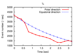
Figure 9: The expected event number of $\bar{\nu}_{e}$ in the SK as a function of the time. The solid line (red line) and the the dotted line (blue line) is for the polar and the equatorial direction, respectively. The supernova is assumed to be located at the distance of 10 kpc. The error bars represent the 1$\sigma$ statistical errors only.

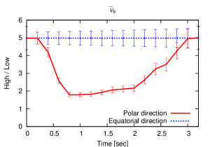
Figure 10: Same as Figure 9, but for the ratio of high- to low-energy events defined in Eq. (3.7).

Here we define a ratio of the high-energy to the low-energy event numbers as in [31]:

$$\mathrm{R(H/L)}=\frac{\mathrm{event}\,\,\mathrm{number}\,\,\mathrm{of}\,\,20<E<60\,\,\mathrm{MeV}}{\mathrm{event}\,\,\mathrm{number}\,\,\mathrm{of}\,\,5<E<20\,\,\mathrm{MeV}}.$$ (40)

It is shown in Figure 10 that the ratio could be a helpful tool to identify the shock effect more clearly.

3.4 Expected event number of $\nu_{e}$ at the Super-Kamiokande detector

Now we proceed to discuss the shock effect on the L-resonance (Figure 3).

In the L-resonance region, the shock influences not $\bar{\nu}_{e}$ but $\nu_{e}$ in the inverted mass hierarchy. We calculate the survival probability of $\nu_{e}$, $P(E_{\nu})$, in the same manner described in Section 2.2. As will be shown below, the qualitative behavior of $\nu_{e}$ in the L-resonance closely resembles to that of $\bar{\nu}_{e}$ in the H-resonance. Just like the case of the H-resonance (section 3.1), the survival probability of $\nu_{e}$ is about 0.3 in absence of the shock, becomes 0.7, when the shock reaches to the L-resonance layer. Also as in the case of $\bar{\nu}_{e}$, the shock effect on the survival probabilities shifts from the low- to high- energy side as the shock propagates outward, leading to the change in the observed spectra of $\nu_{e}$ (Figure 11).

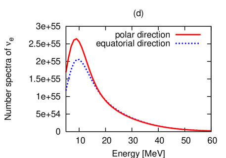
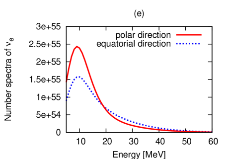
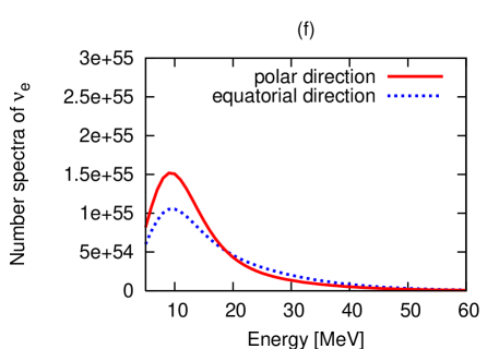
Figure 11: The $\nu_{e}$ spectra in the case of (d), (e) and (f) from top to bottom. We assume the inverted mass hierarchy and $\sin^{2}2\theta_{13}=10^{-3}$.

With these survival probabilities, we calculate the expected event number at the SK for a Galactic source (Figure 13). It can be seen that the event number of the polar direction initially increases and then decreases compared with the one for the equatorial direction, which is due to the increase of the low-energy neutrinos and due to decrease of the high-energy neutrinos, respectively. The event number of $\nu_{e}$ become much fewer than that of $\bar{\nu}_{e}$. This is because the main reaction for detecting $\nu_{e}$ is $\nu_{e}+e^{-}\rightarrow\nu_{e}+e^{-}$, and the cross section is about $10^{-2}$ times smaller than that of $\bar{\nu}_{e}$. Note that the cross section of $\nu_{e}+e^{-}\rightarrow\nu_{e}+e^{-}$ is largest among neutrino-electron scattering reactions (e.g., [65]) and that this forward scattering reaction could be an important tool for identifying the direction to the supernova ([66, 67, 68, 69]). As in the case of the $\bar{\nu}_{e}$, R(H/L) defined in Eq.(40) could be a good probe, especially when the event number is smaller here (Figure 13). The ratio begins to decrease near around $1$ s, which might be an observable signature of the shock entering to the L-resonance. While the statistical errors are eye-catching compared to those of the H-resonance due to the small event numbers here (compare Figure 10), the overlap of the error bars from 1.5 to 2.5s in the high/low-ratio is fortunately small, which could mark a marginally distinguishable feature.

To our knowledge, the possibility of observing the shock feature in the L-resonance has been never claimed before. This is because in the conventional delayed explosion models of core-collapse supernovae, the neutrino oscillation in L-resonance is thought to be minor because the original neutrino luminosity decreases to be so small until the shock wave reaches to the L-resonance. Due to the small cross section of $\nu_{e}$, the detection of the shock effect should not be easy even for the case of magnetic explosions considered here. However we speculate the detection to be more promising when the proposed next-generation megaton-class detectors such as the Hyper-Kamiokande ($\sim$0.5-Mton) [70] and the Deep-TITAND ($\sim$5-Mton) [71] are on-line, possibly making the event number up to two-orders-of-magnitudes higher than for the SK.

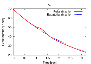
Figure 12: The expected event number of $\nu_{e}$ in the SK as a function of time. The solid line (red line) and the dotted line (blue line) for the polar and equatorial direction, respectively. The supernova is assumed to be located at the distance of 10 kpc.

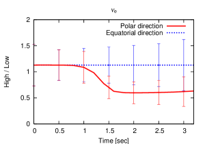
Figure 13: Same as Figure 12, but for the ratio defined in Eq. (3.7). The error bars represent the statistical errors only.

4 Discussion

4.1 Dependence of $\theta_{13}$ on neutrinos

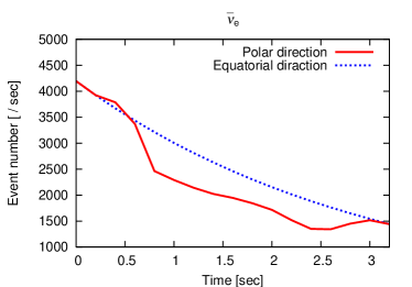
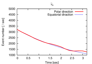
Figure 14: The expected event number of $\bar{\nu}_{e}$ are shown. The expected event number in the left panel are calculated with $\sin^{2}2\theta_{13}=10^{-2}$ and that in the right panel are calculated with $\sin^{2}2\theta_{13}=10^{-5}$. The solid lines (red lines) and the dotted lines (blue lines) are the event number in the polar direction and the equatorial direction, respectively.

First of all, we discuss the dependence of $\theta_{13}$ on the expected event number. Considering the uncertainty of $\theta_{13}$, we calculate the event number changing $\sin^{2}2\theta_{13}=10^{-2}$ and $10^{-5}$ in addition to the fiducial value of $10^{-3}$.

The two panels of Figure 14 show the event number of $\bar{\nu}_{e}$ for $\sin^{2}2\theta_{13}=10^{-2}$ (left) and $10^{-5}$ (right). It can be seen that the event number of $\sin^{2}2\theta_{13}=10^{-2}$ is larger than that of $\sin^{2}2\theta_{13}=10^{-5}$, regardless of the viewing direction. Moreover, the event number for $\sin^{2}2\theta_{13}=10^{-2}$ in the polar direction shows a much steeper shock effect than for $\sin^{2}2\theta_{13}=10^{-5}$. Those features can be understood as follows.

As already mentioned, the change in the event number is sensitive to the adiabaticity condition (e.g., Eq. (22). If $\theta_{13}$ is relatively large (e.g. $\sin^{2}2\theta_{13}=10^{-2},10^{-3}$) and there is no shock wave in the resonance, the adiabatic condition is satisfied for the H-resonance, converting almost all $\bar{\nu}_{x}$ to $\bar{\nu}_{e}$. Since the average energies of neutrinos in the supernova environment are in the following order, $\bar{E}_{\nu_{e}}<\bar{E}_{\bar{\nu}_{e}}<\bar{E}_{\nu_{x},\bar{\nu}_{x}}$, the average energy of $\bar{\nu}_{e}$ becomes higher than the original $\bar{\nu}_{e}$ due to the flavor conversion from $\bar{\nu}_{x}$. On the other hand, if $\theta_{13}$ is small (e.g., $10^{-5}$) or there is a shock wave in the resonance, the adiabatic condition is not satisfied. In this non-adiabatic case in the H-resonance, the original $\bar{\nu}_{e}$ spectrum almost keeps unchanged.

As stated in section 3.3, the cross section for detecting $\bar{\nu}_{e}$ depends on $E_{\nu}^{2}$. Therefore the $\bar{\nu}_{e}$ event number of the adiabatic case becomes larger than that of the non-adiabatic case. If the resonance is closely non-adiabatic always, the shock effect becomes very minor, which is the case for the right panel in Figure 14. We also calculate R(H/L) defined by Eq.(40). In the case of $\sin^{2}2\theta_{13}=10^{-2}$, R(H/L) of $\bar{\nu}_{e}$ is similar to Figure 10. Conversely, the time evolution of R(H/L) of $\bar{\nu}_{e}$ of $\sin^{2}2\theta_{13}=10^{-5}$ does not show the shock feature.

4.2 Difference of the original neutrino spectrum

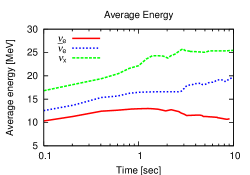
Figure 15: The evolution of average neutrino energies for the time-dependent spectra model [17] (see text for more details). The solid line (red line), dashed line (green line) and the dotted line (blue line) represents the evolution of the average energy of $\nu_{e}$, $\bar{\nu}_{e}$ and $\nu_{x}$, respectively.

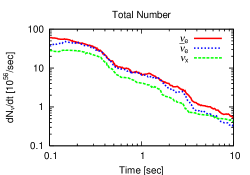
Figure 16: Same as Figure 15, but for the neutrino emission rate as a function of time in Eq. (4.1) (e.g., [17]).

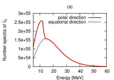
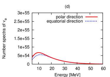
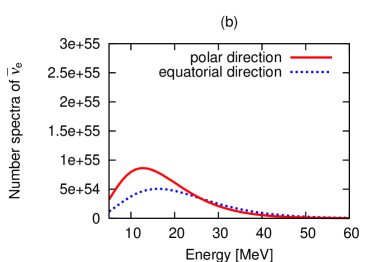
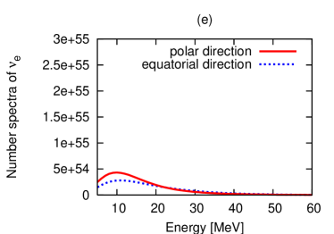
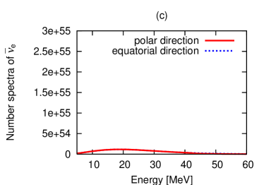
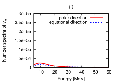
Figure 17: The neutrino spectra in the case of (a)$-$(f) using the time-dependent original spectra. Left panels are spectra of $\bar{\nu}_{e}$, and right figures are $\nu_{e}$. The solid lines (red lines) and the dotted lines (blue lines) are the spectra in the polar direction and the equatorial direction, respectively. We assume $\sin^{2}2\theta_{13}=10^{-3}$ and inverted mass hierarchy.

In this section, we discuss the variations of the original neutrino spectra, and its effect on the obtained results. As already mentioned in section 2.2, we have employed the one, which is assumed to decay exponentially with a timescale of $t_{\rm L}=$ 3 s with the average neutrino energies kept unchanged and is adjusted to be consistent with the total neutrino energies in the model of Lawrence Livermore group [10]. Such a treatment has been often employed so far in the supernova neutrino and nucleosynthesis studies (e.g. Yoshida et al. 2006 [63] and reference therein). When we set $t_{\rm L}$ to be 6 sec, the obtained results are qualitatively unchanged though the event number becomes smaller up to a factor of $\sim$ 2 than for the decay-time of 3 s.

To explore the uncertainty of the original spectra, we here employ another original neutrino spectra used in [17] as follows,

$$\phi^{0}_{\nu}=\frac{dN_{\nu}}{dt}\phi(E_{\nu}),$$ (41)

where $dN_{\nu}/dt$ is a neutrino emission rate, and $\phi(E)$ is a normalized energy spectra defined as,

$$\phi(E_{\nu})=\frac{(\alpha+1)^{\alpha+1}}{\Gamma(\alpha+1)}\left(\frac{E_{\nu}}{\langle E_{\nu}\rangle}\right)^{\alpha}\frac{e^{-(\alpha+1)E_{\nu}/\langle E_{\nu}\rangle}}{\langle E_{\nu}\rangle}.$$ (42)

$\langle E\rangle$, $\alpha$, and $\Gamma$ is the average energy, an energy shape parameter, and the gamma function, respectively [17]. For simplicity, we have taken $\alpha=3$ for all flavors [30]. In this model, $\frac{dN_{\nu}}{dt}$ and $\langle E\rangle$ follow the calculation of the Lawrence Livermore group [10]. The time evolution of the average energy and the neutrino emission rate is shown in Figure 16 and 16, respectively. The solid line (red line), the dashed line (green line) and the dotted line (blue line) corresponding that of $\nu_{e}$, $\bar{\nu}_{e}$ and $\nu_{x}$, respectively. Hereafter we call this spectra as “time-dependent” original spectra.

Figure 17 shows the neutrino spectra at the SK calculated by the mentioned procedure in section 3.3, in which left and light panel is for $\bar{\nu}_{e}$ and $\nu_{e}$, respectively. It can be shown that the neutrino spectra are qualitatively insensitive to the difference in the original neutrino spectra examined here. However significant difference appears in the event number. Figure 19 and 19 is the event number of $\bar{\nu}_{e}$ and $\nu_{e}$, respectively. The difference of the event number between the polar and the equatorial direction becomes much smaller than that of our fiducial model shown in Figures 10 and 13. This is because the neutrino flux of the time-dependent spectra decreases already before the shock reaches to the resonance layers.

R(H/L) is shown in Figures 21 (for $\bar{\nu}_{e}$) and 21 (for $\nu_{e}$). In the equatorial direction of Figure 21, the ratio gradually increases although it is constant in Figure 10. This reflects the increase of the average energy of $\bar{\nu}_{e}$ with time (see the dotted line of Figure 16). In contrast, the ratio of the equatorial direction is almost flat in Figure 21, reflecting the evolution of the average energy of $\nu_{e}$. The error bars here are shown to be larger than for Figure 13, simply because the event number of $\nu_{e}$ here becomes smaller than for the original neutrino spectrum in section 2.2 (compare Figure 12 with 19). Albeit sensitive to the feature of the original spectra, it is found that the ratio for the polar direction becomes generally smaller than for the equatorial direction due to the shock effect (Figures 10, 20, 21) for relatively large value of $\theta_{13}$.

Those results indicate that the shock effect on the event number discussed so far, is subject to the large uncertainty of the original neutrino spectra. What is qualitatively new pointed out in this paper is that in the MHD explosions, the timescale of the shock-arrival could be shorter than the decay timescale of the neutrino flux, albeit depending on the evolution of the neutrino spectra. It should be also mentioned that if the energy difference between $\bar{\nu}_{e}$ and $\nu_{x}$ becomes small due to detailed neutrino interactions near the neutrinosphere [72, 73], the shock effect should be also small. To determine the original neutrino spectra in a consistent manner with the shock-dynamics in the supernova envelope requires more sophisticated MHD modeling of core-collapse supernova, in which detailed microphysics is also included. Several groups are really pursuing it with the use of advanced numerical techniques [46, 47], however still unfeasible at present.

In this paper, we neglected the effect of neutrino self-interactions. Among a number of important effects possibly created by self-interactions (e.g.,[29, 36]), we choose to consider the effect of single spectral swap of $\bar{\nu}_{e}$ and $\nu_{x}$ suggested by Fogli et al. [74]. In our model, the original spectrum was $\phi_{\bar{\nu}_{e}}>\phi_{\nu_{x}}$ in the low-energy side, and $\phi_{\bar{\nu}_{e}}<\phi_{\nu_{x}}$ in the high-energy side. Due to the spectral swap, the above inequality sign reserves. Thus the influence of the shock should occur also oppositely (see Eq.(39) and discussion in section 3.2). Therefore the event number of neutrinos in the polar direction is expected to increase by the influence of the shock. To draw a robust conclusion to the self-interaction effects on our models naturally requires more sophisticated analysis (e.g., [34]), which we pose as a next step of this study.

As a prelude to more realistic computations of the flavor conversions taking into account the effects of neutrino self-interaction, also with more realistic input of the neutrino spectra, our findings obtained in a very idealized modeling should be the very first step towards the prediction of the neutrino signals from magnetic explosions of massive stars.

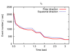
Figure 18: The expected event number of $\bar{\nu}_{e}$ using the time-dependent original spectra. The solid lines (red lines) and the dotted lines (blue lines) are the event number for the polar and equatorial direction, respectively. The source is assumed to be at $10$ kpc.

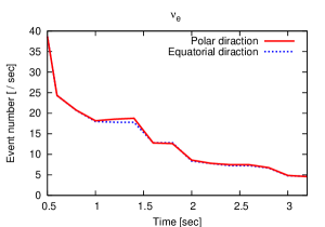
Figure 19: Same as Figure 18 but for $\nu_{e}$.

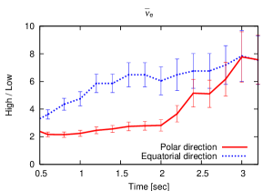
Figure 20: The ratio of event number of $\bar{\nu}_{e}$ using the time-dependent original spectra. The solid lines (red lines) and the dotted lines (blue lines) are the event number in polar direction and equatorial direction, respectively.

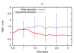
Figure 21: Same as Figure 20 but for $\nu_{e}$.

5 Summary

We studied neutrino oscillations from core-collapse supernovae that produce magnetohydrodynamic (MHD) explosions, which are attracting great attention recently as a possible relevance to magnetars and/or long-duration gamma-ray bursts. Based on a recent supernova simulation producing MHD explosions till the shock break-out, we calculated numerically the flavor conversion in the highly non-spherical envelope through the pure matter-driven MSW effect. As for the neutrino spectra at the neutrino sphere which the MHD simulations lack, we employed the two variations based on the Lawrence Livermore simulation, with or without the evolution of the average neutrino energies. With these computations, we investigated how the explosion anisotropy could have impacts on the emergent neutrino spectra and also on the observed neutrino event number at the Super-Kamiokande detector for a Galactic supernova.

In the case of the inverted mass hierarchy with a relatively large $\theta_{13}$ ($\sin^{2}2\theta_{13}\gtrsim 10^{-3}$), we demonstrated that survival probabilities of $\bar{\nu}_{e}$ and $\nu_{e}$ seen along the rotational axis of the MHD supernovae (i.e., polar direction), could be significantly different from those seen from the equatorial direction. The event numbers of $\bar{\nu}_{e}$ observed from the polar direction show steepest decrease, reflecting the passage of the magneto-driven shock to the so-called high-resonance regions. We pointed out that such a shock effect, depending on the original neutrino spectra, appears also for the low-resonance regions, which could lead to a noticeable decrease in the $\nu_{e}$ signals. This reflects a unique nature of the magnetic explosion featuring a very early shock-arrival to the resonance regions, which is in sharp contrast to the delayed neutrino-driven supernova models in spherical symmetry. Our results suggested that the two features in the $\bar{\nu}_{e}$ and $\nu_{e}$ signals, if visible to the Super-Kamiokande for a Galactic supernova, could be an observational signature of magneto-driven supernovae.

One of the nearest supernovae, associated with the long-duration gamma-ray burst (GRB) is, SN1998bw (Type Ic) at the distance of $\sim 14$ Mpc [58]. As mentioned earlier, such events are likely to be associated with the energetic stellar explosions induced by magnetic mechanisms, often referred to as hypernovae (e.g., [75] and references therein). It is interesting to note that the fraction of SNe Ib/c associated with long GRBs is small ($\sim 1\%-10\%$), however, is appeared to coincide with that of hypernovae. Albeit with large uncertainties of GRB statistics, the link between hypernovae and long GRBs seems to be observationally supported (see discussion in [76] and reference therein). Recently the proposals of Mton-class detectors such as Hyper-Kamiokande [70] and Deep-TITAND [71], are becoming a real possibility, by which the shock effect studied here could be visible out to the Megaparsec distance scales. This implies that the shock effect, if observed (much nicer if observed also by the electromagnetic and gravitational-wave observations [77, 78]), could provide important hints to understand the long-veiled central engines of gamma-ray bursts, because the shock arrival time to resonance layers should reflect the activities of the engine. We hope that this study could give strong momentum to theorists for making more precise predictions of the neutrino signals from magneto-driven supernovae.

- [1] S. Ando, J. F. Beacom and H. Yuksel, Detection of neutrinos from supernovae in nearby galaxies, Phys. Rev. Lett. 95 (2005) 171101
- [2] A. Heger, C. L. Fryer, S. E. Woosley, N. Langer and D. H. Hartmann, How Massive Single Stars End their Life Astrophys. J. 591 (2003) 288
- [3] K. Hirata, Y. Kajita, M. Koshiba, M. Nakahata and Y. Oyama, Observation of a Neutrino Burst from the Supernova SN 1987a, Phys. Rev. Lett. 58 (1987) 1490
- [4] R. M. Bionta, G. Blewitt, C. B. Bratton, D. Caspere and A. Ciocio, Observation of a Neutrino Burst in Coincidence with Supernova SN 1987a in the Large Magellanic Cloud, Phys. Rev. Lett. 58 (1987) 1494
- [5] K. Sato and H. Suzuki, Analysis Of Neutrino Burst From The Supernova In Lmc. Phys. Rev. Lett. 58 (1987) 2722
- [6] H. Suzuki and K. Sato, Statistical Analysis Of The Neutrino Burst From Sn1987a, Prog. Theor. Phys. 79 (1988) 725
- [7] G. G. Raffelt, Physics with supernovae Nucl. Phys. 110 (Proc. Suppl.) (2002) 254
- [8] Y. Totsuka, Neutrino astronomy Rept. Prog. Phys. 55 (1992) 377
- [9] KamLAND Collaboration, A. Suzuki et al., Present Status of KamLAND, Nucl. Phys. 77 (Proc. Suppl.) (1999) 171
- [10] T. Totani, K. Sato, H. E. Dalhed and J. R. Wilson, Future detection of supernova neutrino burst and explosion mechanism, Astrophys. J. 496 (1998) 216 [astro-ph/9710203]
- [11] J. F. Beacom, Supernovae and neutrinos, Nucl. Phys. 118 (Proc. Suppl.) (2003) 307 [astro-ph/0209136]
- [12] A. S. Dighe and A. Y. Smirnov, Identifying the neutrino mass spectrum from a supernova neutrino burst, Phys. Rev. D 62 (2000) 033007 [hep-ph/9907423].
- [13] G. Fogli, E. Lisi, D. Montanino and A. Palazzo, Identifying the neutrino mass spectrum from the neutrino burst from a supernova. Phys. Rev. D 65 (2002) 073008 [hep-ph/9907423].
- [14] C. Lunardini and A. Yu. Smirnov Probing the neutrino mass hierarchy and the 13-mixing with supernovae JCAP 0306 (2003) 009 [hep-ph/0302033]
- [15] A. S. Dighe, M. T. Keil and G. G. Raffelt, Detecting the neutrino mass hierarchy with a supernova at IceCube JCAP 0306 (2003) 005 [hep-ph/0303210].
- [16] K. Takahashi, M. Watanabe, K. Sato and T. Totani, Effects of neutrino oscillation on the supernova neutrino spectrum, Phys. Rev. D 64 (2001) 093004 [hep-ph/0105204].
- [17] G. Fogli, E. Lisi, A. Mirizzi and D. Montanino, Probing supernova shock waves and neutrino flavor transitions in next-generation water-Cherenkov detectors, JCAP 0504 (2005) 002 [hep-ph/0412046].
- [18] J. F. Beacom and P. Vogel, Mass signature of supernova nu/mu and nu/tau neutrinos in SuperKamiokande Phys. Rev. D 58 (1998) 053010
- [19] K. Kotake, K. Sato and K. Takahashi, Explosion Mechanism, Neutrino Burst, and Gravitational Wave in Core-Collapse Supernovae Rept. Prog. Phys. 69 (2006) 971 [astro-ph/0509456].
- [20] S. P. Mikheev and A. Y. Smirnov, Resonance Amplification of Oscillations in Matter and Spectroscopy of Solar Neutrinos, Sov. J. Nucl. Phys. 42 (1985) 913 [Yad. Fiz. 42 (1985) 1441].
- [21] S. P. Mikheev and A. Y. Smirnov, Neutrino oscillations in a variable density medium and bursts due to the gravitational collapse of stars, Sov. Phys. JETP 64 (1986) 4 [Zh. Eksp. Teor. Fiz. 91 (1986) 7].
- [22] A. B. Balantekin, J. M. Fetter and F. N. Loreti, The MSW effect in a fluctuating matter density, Phys. Rev. D 54 (1996) 3941 [astro-ph/9604061]
- [23] K. Takahashi, K. Sato, A. Burrows and T. A. Thompson, Supernova neutrinos, neutrino oscillations, and the mass of the progenitor star, Phys. Rev. D 68 (2003) 113009 [hep-ph/0306056].
- [24] M. Kachelriess, R. Tomas, R. Buras, H. T. Janka, A. Marek, and M. Rampp, Exploiting the neutronization burst of a galactic supernova Phys. Rev. D 71 (2005) 063003 [astro-ph/0412082].
- [25] C. Lunardini and A. Y. Smirnov, Supernova neutrinos: Earth matter effects and neutrino mass spectrum Nucl. Phys. B 616 (2001) 307 [hep-ph/0106149]
- [26] A. S. Dighe, M. Kachelriess, G. G. Raffelt and R. Tomas, Signatures of supernova neutrino oscillations in the earth mantle and core, JCAP 0401 (2004) 004 [hep-ph/0311172].
- [27] R. C. Schirato and G. M. Fuller Connection between supernova shocks, flavor transformation, and the neutrino signal [astro-ph/0205390]
- [28] C. Lunardini, B. Mller and H. Th. Janka, Neutrino oscillation signatures of oxygen-neon-magnesium supernovae, Phys. Rev. D 78 (2008) 023016 [\arXivid0712.3000]
- [29] H. Duan and J. P. Kneller, Neutrino flavor transformation in supernovae [\arXivid0904.0974].
- [30] R. Toms, M. Kachelrie, G. Raffelt, A. Dighe, H. T. Janka and L. Scheck, Neutrino signatures of supernova shock and reverse shock propagation, JCAP 0409 (2004) 015 [astro-ph/0407132].
- [31] K. Takahashi, K. Sato, H. E. Dalhed and J. R. Wilson, Shock propagation and neutrino oscillation in supernova, Astropart. Phys. 20 (2003) 189 [astro-ph/0212195].
- [32] G. G. Raffelt and A. Y. Smirnov, Self-induced spectral splits in supernova neutrino fluxes, Phys. Rev. D 76 (2007) 081301 [\arXivid0705.1830].
- [33] H. Duan, G. M. Fuller and J. Carlson, Simulating nonlinear neutrino flavor evolution [\arXivid0803.3650].
- [34] B. Dasgupta and A. Dighe, Collective three-flavor oscillations of supernova neutrinos Phys. Rev. D 77 (2008) 113002 [arXiv:0712.3798 [hep-ph]].
- [35] B. Dasgupta, A. Dighe and A. Mirizzi, Identifying neutrino mass hierarchy at extremely small theta(13) through Earth matter effects in a supernova signal Phys. Rev. Lett. 101 (2008) 171801 [arXiv:0802.1481 [hep-ph]].
- [36] H. Duan, G. M. Fuller and Y. Z. Qian, Collective neutrino flavor transformation in supernovae, Phys. Rev. D 74 (2006) 123004 [astro-ph/0511275].
- [37] C. S. Lim and W. J. Marciano, Resonant Spin - Flavor Precession of Solar and Supernova Neutrinos, Phys. Rev. D 37, 1368 (1988). Phys. Rev. D 37 (1988) 1368.
- [38] E. K. Akhmedov, Resonant Amplification of Neutrino Spin Rotation in Matter and the Solar Neutrino Problem, Phys. Lett. B 213, 64 (1988). Phys. Lett. B 213 (1988) 64.
- [39] E. K. Akhmedov and T. Fukuyama, Supernova prompt neutronization neutrinos and neutrino magnetic moments. JCAP 0312 (2003) 007 [hep-ph/0310119]
- [40] S. Ando and K. Sato, Resonant spin flavor conversion of supernova neutrinos: Dependence on presupernova models and future prospects. Phys. Rev. D 68 (2003) 023003 [hep-ph/0305052]
- [41] T. Totani & K. Sato, Resonant spin-flavor conversion of supernova neutrinos and deformation of the electron antineutrino spectrum , Phys. Rev. D 54 (1996) 5975 [astro-ph/9609035]
- [42] L. Wang, D. A. Howell, P. Hoeflich and J. C. Wheeler, Bi-polar Supernova Explosions Astrophys. J. 550 (2001) 1030 [astro-ph/9912033].
- [43] A. Marek and H. T. Janka, Delayed neutrino-driven supernova explosions aided by the standing accretion-shock instability Astrophys. J. 694 (2009) 664 [\arXivid0708.33372].
- [44] W. Iwakami, K. Kotake, N. Ohnishi, S. Yamada and K. Sawada, Three-Dimensional Simulations of Standing Accretion Shock Instability in Core-Collapse Supernovae, Astrophys. J. 678 (2008) 1207 [\arXivid0710.2191].
- [45] K. Kotake, K. Sato, H. Sawai and S. Yamada, Magnetorotational effects on anisotropic neutrino emission and convection in core-collapse supernovae Astrophys. J. 608 (2004) 391
- [46] A. Burrows, L. Dessart, E. Livne, C. D. Ott and J. Murphy, Simulations of Magnetically-Driven Supernova and Hypernova Explosions in the Context of Rapid Rotation, [astro-ph/0702539].
- [47] T. Takiwaki, K. Kotake and K. Sato, Special Relativistic Simulations of Magnetically-dominated Jets in Collapsing Massive Stars Astrophys. J. 691 (2009) 1360 [\arXivid0712.1949].
- [48] A. Burrows, E. Livne, L. Dessart, C. Ott and J. Murphy, A New Mechanism for Core-Collapse Supernova Explosions, Astrophys. J. 640 (2006) 878 [astro-ph/0510687].
- [49] A. Friedland and A. Gruzinov, Neutrino signatures of supernova turbulence [astro-ph/0607244]. arXiv:astro-ph/0607244.
- [50] S. Choubey, N. P. Harries and G. G. Ross, Turbulent supernova shock waves and the sterile neutrino signature in megaton water detectors, Phys. Rev. D 76 (2007) 073013 [hep-ph/0703092]
- [51] J. P. Kneller, G. C. McLaughlin and J. Brockman, Oscillation Effects and Time Variation of the Supernova Neutrino Signal, Phys. Rev. D 77 (2008) 045023 [\arXivid0705.3835].
- [52] N. Bucciantini, E. Quataert, J. Arons, B. D. Metzger and T. A. Thompson, Relativistic Jets and Long-Duration Gamma-ray Bursts from the Birth of Magnetars, MNRAS 383 (2008) 383 [\arXivid0707.2100].
- [53] A. MacFadyen and S. E. Woosley, Collapsars - Gamma-Ray Bursts and Explosions in ”Failed Supernovae”, Astrophys. J. 524 (1999) 262 [astro-ph/9810274].
- [54] S. Nagataki, R. Takahashi, A. Mizuta and T. Takiwaki, Numerical study of gamma-ray burst jet formation in collapsars, Astrophys. J. 659 (2007) 512.
- [55] S. Harikae, T. Takiwaki and K. Kotake, Long-Term Evolution of Slowly Rotating Collapsar in Special Relativistic Magnetohydrodynamics [\arXivid0905.2006].
- [56] T. Piran, The physics of gamma-ray bursts Rev. Mod. Phys. 76, 1143 (2004) [astro-ph/0405503].
- [57] A. Heger, N. Langer and S. E. Woosley, Presupernova evolution of rotating massive stars. 1. Numerical method and evolution of the internal stellar structure, Astrophys. J. 528 (2000) 368 [astro-ph/9904132]
- [58] T. J. Galama et al. Discovery of the peculiar supernova 1998bw in the error box of GRB 980425 Nature 395 (1998) 670 [astro-ph/9806175]
- [59] S. Woosley and A. Heger, The Progenitor Stars of Gamma-Ray Bursts, Astrophys. J. 637 (2006) 914 [astro-ph/0508175].
- [60] M. Obergaulinger, M. A. Aloy and E. Muller, Axisymmetric simulations of magneto–rotational core collapse: dynamics and gravitational wave signal, Astron. Astrophys. 450 (2006) 1107 [astro-ph/0510184]
- [61] M. Fukugita and T. Yanagida, 2003, Physics of Neutrinos and Applications to Astrophysics, Springer, Berlin.
- [62] M. Maltoni, T. Schwetz, M. A. Tortola and J. W. F. Valle, Status of global fits to neutrino oscillations, New J. Phys. 6 (2004) 122 [hep-ph/0405172].
- [63] T. Yoshida, T. Kajino, H. Yokomakura, K. Kimura, A. Takamura and D. H. Hartmann, Neutrino Oscillation Effects on Supernova Light Element Synthesis, Astrophys. J. 649 (2006) 319 [astro-ph/0606042].
- [64] M. B. Smy, Low Energy Challenges in Super-Kamiokande-III, Nucl. Phys. 168 (Proc. Suppl.) (2007) 118
- [65] Hirata, K. S., et al. Observation in the Kamiokande-II detector of the neutrino burst from supernova SN1987A, Phys. Rev. D 38 (1988) 448
- [66] M. Nakahata, Supernova Neutrinos and Recent Results from Supernova-Kamiokande, Proceedings of the Yamada Conference LIX on Inflating Horizons of Particle Astrophysics and Cosmology (H.Suzuki, J.Yokoyama, Y.Suto, and K. Sato, Japan, 2006, pp 29 - 37)
- [67] A. Burrows, D. Klein and R. Gandhi The Future of supernova neutrino detection, Phys. Rev. D 45 (1992) 3361
- [68] J. F. Beacom and P. Vogel, Can a supernova be located by its neutrinos?, Phys. Rev. D 60 (1999) 033007, [astro-ph/9811350].
- [69] R. Tomas, D. Semikoz, G. G. Raffelt, M. Kachelriess and A. S. Dighe, Supernova pointing with low- and high-energy neutrino detectors, Phys. Rev. D 68 (2003) 093013, [hep-ph/0307050].
- [70] K. Nakamura, Hyper-Kamiokande: A next generation water Cherenkov detector, Int. J. Mod. Phys. A 18 (2003) 4053.
- [71] Y. Suzuki et al. [TITAND Working Group], Multi-Megaton water Cherenkov detector for a proton decay search: TITAND [hep-ex/0110005].
- [72] G. G. Raffelt, Muon-neutrino and tau-neutrino spectra formation in supernovae, Astrophys. J. 561 (2001) 890 [astro-ph/0105250].
- [73] M. T. Keil, G. G. Raffelt and H. T. Janka, Monte Carlo study of supernova neutrino spectra formation, Astrophys. J. 590 (2003) 971 [astro-ph/0208035].
- [74] G. L. Fogli, E. Lisi, A. Marrone and A. Mirizzi, Collective neutrino flavor transitions in supernovae and the role of trajectory averaging, JCAP 0712 (2007) 010 [\arXivid0707.1998].
- [75] M. Tanaka et al., Spectropolarimetry of the Unique Type Ib Supernova 2005bf: Larger Asymmetry Revealed by Later-Phase Data [astro-ph/0906.1062].
- [76] C. L Fryer et al. Constraints on Type Ib/c Supernovae and Gamma-Ray Burst Progenitors, PASP 119 (2007) 1211.
- [77] K. Kotake, W. Iwakami, N. Ohnishi and S. Yamada, Stochastic Nature of Gravitational Waves from Supernova Explosions with Standing Accretion Shock Instability Astrophys. J. 697 (2009) L133 [astro-ph/0904.4300]
- [78] C. D. Ott, The gravitational-wave signature of core-collapse supernovae, Class. and Quant. Grav. 26 (2009) 063001 [\arXivid0809.0695].