Calibrating passive scalar transport in shear-flow turbulence

Abstract

The turbulent diffusivity tensor is determined for linear shear flow turbulence using numerical simulations. For moderately strong shear, the diagonal components are found to increase quadratically with Peclet and Reynolds numbers below about 10 and then become constant. The diffusivity tensor is found to have components proportional to the symmetric and antisymmetric parts of the velocity gradient matrix, as well as products of these. All components decrease with the wave number of the mean field in a Lorentzian fashion. The components of the diffusivity tensor are found not to depend significantly on the presence of helicity in the turbulence. The signs of the leading terms in the expression for the diffusion tensor are found to be in good agreement with estimates based on a simple closure assumption.

I Introduction

In a turbulent flow, chemicals tend to be mixed more effectively than in the absence of turbulence. Indeed, turbulence disperses chemicals by advecting particles along chaotic trajectories. This rapidly causes large concentration gradients that speed up their mixing down toward the smallest scales. Turbulent mixing is a complicated and rich process; see Ref. FGV01 for a comprehensive review on this subject. The mathematical treatment of the description of turbulent mixing is closely related to that of turbulence itself, but it is in many ways much simpler and provides therefore an ideal tool for making conceptual progress in that field SS00 .

Here we are mainly interested in cases where it is meaningful to define a mean concentration whose scale of variation is large compared with the scale of the energy-carrying eddies. In such cases it can be useful to describe the change in the mean concentration by an effective turbulent diffusion tensor. On smaller scales the change in the mean concentration can still be described in such a way, but in that case the multiplication with a turbulent diffusivity must be replaced with a convolution. The turbulent diffusion tensor quantifies the effective exchange of chemicals or other passive scalar quantities advected by the flow. If there is a gradient in the mean concentration $\overline{C}$ of chemicals, there will be a net mean flux $\overline{\mbox{\boldmath${\cal F}$}}{}=\overline{\mathchoice{\mbox{\boldmath$\displaystyle u$}}{\mbox{\boldmath$\textstyle u$}}{\mbox{\boldmath$\scriptstyle u$}}{\mbox{\boldmath$\scriptscriptstyle u$}}{}c}$ of chemicals resulting from a systematic correlation of fluctuations in the concentration $c$ and the turbulent velocity $\textstyle u$. Here, overbars denote averaging. Under isotropic conditions with sufficient scale separation, this mean flux will be down the gradient of concentration, with

$$\overline{\mbox{\boldmath${\cal F}$}}{}=-\kappa_{\rm t}\mathchoice{\mbox{\boldmath$\displaystyle\nabla$}}{\mbox{\boldmath$\textstyle\nabla$}}{\mbox{\boldmath$\scriptstyle\nabla$}}{\mbox{\boldmath$\scriptscriptstyle\nabla$}}{}\overline{C},$$ (1)

where $\kappa_{\rm t}$ is the turbulent diffusivity. However, modifications are expected when the turbulence is anisotropic. In that case this relation takes the form

$$\overline{\cal F}_{i}=-\kappa_{ij}\nabla_{j}\overline{C},$$ (2)

where $\kappa_{ij}$ is now the turbulent diffusion tensor. In this paper we are interested in the anisotropy caused by the presence of shear. One of the results one expects to see is a suppression of turbulent transport in the cross-stream direction. This effect is discussed in various physical circumstances such as geophysical flows Ter00 , turbulent plasmas Bur97 , and solar physics Kim05 ; LK06 .

Much of this research is done using analytical techniques such as the first-order smoothing approximation and the renormalization group analysis. However, in recent years it has become possible to calculate turbulent transport coefficients using numerical realizations of turbulence from direct simulations. Turbulent transport coefficients can then be determined by imposing a gradient in the passive scalar concentration and measuring the resulting concentration fluxes BKM04 . By imposing gradients in three different directions it is possible to assemble all components of the turbulent diffusion tensor.

In recent years such a technique has been applied to the case of magnetic fields whose evolution is controlled not just by turbulent magnetic diffusion, but also by non-diffusive contributions known as the $\alpha$ effect Sch05 ; Sch07 . In this way it has been possible to investigate numerically the effects of shear and rotation in regimes that cannot be treated analytically. The technique is known under the name test-field method, which refers to the fact that this approach involves the analysis of correlations for a set of different pre-determined test fields. In the analogous case of passive scalars, this method is now often referred to as test-scalar method BSV09 .

Using this method, it has recently been possible to determine the turbulent diffusion tensor in cases where the turbulence is anisotropic owing to the presence of either rotation or an imposed magnetic field BSV09 . In the case of rotation the angular velocity vector $\textstyle\Omega$ provides a new element for constructing an anisotropic rank-2 tensor of the form KRP94

$$\kappa_{ij}=\kappa_{0}\delta_{ij}+\kappa_{\Omega}\epsilon_{ijk}\hat{\Omega}_{k}+\kappa_{\Omega\Omega}\hat{\Omega}_{i}\hat{\Omega}_{j},$$ (3)

where $\hat{\bm{\Omega}}=\mathchoice{\mbox{\boldmath$\displaystyle\Omega$}}{\mbox{\boldmath$\textstyle\Omega$}}{\mbox{\boldmath$\scriptstyle\Omega$}}{\mbox{\boldmath$\scriptscriptstyle\Omega$}}{}/|\mathchoice{\mbox{\boldmath$\displaystyle\Omega$}}{\mbox{\boldmath$\textstyle\Omega$}}{\mbox{\boldmath$\scriptstyle\Omega$}}{\mbox{\boldmath$\scriptscriptstyle\Omega$}}{}|$ is the unit vector along the rotation axis and $\kappa_{0}$, $\kappa_{\Omega}$, and $\kappa_{\Omega\Omega}$ are functions of the flow parameters. Note that $\Omega$ is a pseudo vector while $\kappa_{ij}$ is a proper tensor, so all three coefficients in Eq. (3) are proper scalars. In the case of a shear flow, an obvious possible ansatz is obtained by replacing $\textstyle\Omega$ with the vorticity $\overline{\bm{W}}=\mathchoice{\mbox{\boldmath$\displaystyle\nabla$}}{\mbox{\boldmath$\textstyle\nabla$}}{\mbox{\boldmath$\scriptstyle\nabla$}}{\mbox{\boldmath$\scriptscriptstyle\nabla$}}{}\times\overline{\bm{U}}$, which is also a pseudovector (or axial vector), and $\overline{\bm{U}}$ is the mean shear flow. However, such an ansatz would be incomplete, because it only captures the antisymmetric part of the velocity gradient matrix $\overline{U}_{i,j}$, where a comma denotes partial differentiation. A more natural approach would therefore be to invoke both symmetric and antisymmetric parts of the velocity gradient matrix by writing it as $\overline{U}_{i,j}=\overline{\mathsf{S}}_{ij}+\overline{\mathsf{A}}_{ij}$, where

$$\overline{\mathsf{S}}_{ij}={\textstyle{1\over 2}}(\overline{U}_{i,j}+\overline{U}_{j,i}),$$ (4)

$$\overline{\mathsf{A}}_{ij}={\textstyle{1\over 2}}(\overline{U}_{i,j}-\overline{U}_{j,i}).$$ (5)

The latter can also be written as $\overline{\mathsf{A}}_{ij}=-{\textstyle{1\over 2}}\epsilon_{ijk}\overline{W}_{k}$. A proper rank-2 tensor can then be expressed as

$$\kappa_{ij}=\kappa_{\rm t}\delta_{ij}+\kappa_{\sf S}\overline{\sf S}_{ij}+\kappa_{\sf A}\overline{\sf A}_{ij}+\kappa_{{\sf S}{\sf S}}(\overline{\mbox{\boldmath${\mathsf{S}}$}}{}\,\overline{\mbox{\boldmath${\mathsf{S}}$}}{})_{ij}+\kappa_{{\sf A}{\sf S}}(\overline{\mbox{\boldmath${\mathsf{A}}$}}{}\,\overline{\mbox{\boldmath${\mathsf{S}}$}}{})_{ij},$$ (6)

where $\kappa_{\rm t}$, $\kappa_{\sf S}$, $\kappa_{\sf A}$, $\kappa_{{\sf S}{\sf S}}$, and $\kappa_{{\sf A}{\sf S}}$ are proper scalars that are again functions of the flow parameters. In the absence of helicity, no further rank-2 tensors can be constructed from a linear shear flow. We return to the case with helicity in Sec. III.4.

An important goal of this work is to determine the coefficients in Eq. (6) for a linear shear flow of the form

$$\overline{\bm{U}}=(0,Sx,0),$$ (7)

where $S={\rm const}{}$ is the shear rate, which is not to be confused with the tensor $\overline{\mbox{\boldmath${\mathsf{S}}$}}{}$. For a linear shear flow given by Eq. (7), the tensors $\overline{\mbox{\boldmath${\mathsf{S}}$}}{}$ and $\overline{\mbox{\boldmath${\mathsf{A}}$}}{}$ are constants, and their only non-vanishing components are

$$\overline{\mathsf{S}}_{xy}=\overline{\mathsf{S}}_{yx}=-\overline{\mathsf{A}}_{xy}=\overline{\mathsf{A}}_{yx}=S/2.$$ (8)

Note also that

$$\overline{\mbox{\boldmath${\mathsf{S}}$}}{}^{2}=-\overline{\mbox{\boldmath${\mathsf{A}}$}}{}^{2}=(S/2)^{2}\,{\rm diag}\,{}(1,1,0),$$ (9)

$$\overline{\mbox{\boldmath${\mathsf{A}}$}}{}\,\overline{\mbox{\boldmath${\mathsf{S}}$}}{}=-\overline{\mbox{\boldmath${\mathsf{S}}$}}{}\,\overline{\mbox{\boldmath${\mathsf{A}}$}}{}=(S/2)^{2}\,{\rm diag}\,{}(-1,1,0).$$ (10)

With these preparations we can now express all nine components of $\kappa_{ij}$ in terms of the five coefficients in Eq. (6) as follows:

$$\kappa_{11}=\kappa_{\rm t}+{\textstyle{1\over 4}}S^{2}(\kappa_{{\sf S}{\sf S}}-\kappa_{{\sf A}{\sf S}}),$$ (11)

$$\kappa_{22}=\kappa_{\rm t}+{\textstyle{1\over 4}}S^{2}(\kappa_{{\sf S}{\sf S}}+\kappa_{{\sf A}{\sf S}}),$$ (12)

$$\kappa_{33}=\kappa_{\rm t},$$ (13)

$$\kappa_{12}={\textstyle{1\over 2}}S(\kappa_{\sf S}-\kappa_{\sf A}),$$ (14)

$$\kappa_{21}={\textstyle{1\over 2}}S(\kappa_{\sf S}+\kappa_{\sf A}),$$ (15)

$$\kappa_{13}=\kappa_{31}=\kappa_{23}=\kappa_{32}=0.$$ (16)

Given that all nine components of $\kappa_{ij}$ can be determined from simulation data using the test-scalar method, we can use the relations above to compute the five unknown coefficients in Eq. (6) via

$$\kappa_{\sf S}S=\kappa_{21}+\kappa_{12},\quad\kappa_{\sf A}S=\kappa_{21}-\kappa_{12},$$ (17)

$$\kappa_{{\sf S}{\sf S}}S^{2}/2=\kappa_{22}+\kappa_{11}-2\kappa_{33},$$ (18)

$$\kappa_{{\sf A}{\sf S}}S^{2}/2=\kappa_{22}-\kappa_{11},$$ (19)

$$\kappa_{\rm t}=\kappa_{33}.$$ (20)

Note that combinations such as $\kappa_{\sf S}S$ and $\kappa_{{\sf S}{\sf S}}S^{2}/2$ have still the same dimension as $\kappa_{ij}$, so in the following we shall quote these combinations in that form.

In principle it is possible to construct $\kappa_{ij}$ using also the velocity vector $\overline{\bm{U}}$ itself. However, $\overline{\bm{U}}$ varies in $x$ and vanishes at $x=0$. On the other hand, we expect the components of $\kappa_{ij}$ not to depend explicitly on position, making a construction in terms of $\overline{\bm{U}}$ less favorable. Furthermore, the tensor $\overline{U}_{i}\overline{U}_{j}$, which has only one component in the $yy$ position, can already be constructed from $\overline{\mbox{\boldmath${\mathsf{S}}$}}{}^{2}-\overline{\mbox{\boldmath${\mathsf{A}}$}}{}\,\overline{\mbox{\boldmath${\mathsf{S}}$}}{}={\rm diag}\,{}(0,2,0)$, so no new information would be added. However, this changes when we also admit helical turbulent flows, because then there could be tensors of the form $\overline{W}_{i}\overline{U}_{j}$ and $\overline{W}_{j}\overline{U}_{i}$ which have components in the $yz$ and $zy$ directions. For this reason we shall also investigate helical turbulence in some cases.

A comment regarding the case of rotation without shear is here in order. In hindsight it might have been more natural to write Eq. (3) in terms of the antisymmetric matrix $\overline{\mathsf{A}}_{ij}=-{\textstyle{1\over 2}}\epsilon_{ijk}\hat{\Omega}_{k}$, i.e.

$$\kappa_{ij}=\kappa_{\rm t}^{\Omega}\delta_{ij}+\kappa^{\Omega}_{\sf A}\overline{\sf A}_{ij}+\kappa^{\Omega}_{{\sf A}{\sf A}}(\overline{\mbox{\boldmath${\mathsf{A}}$}}{}^{2})_{ij},$$ (21)

with coefficients that are related to those in Eq. (3) via

$$\kappa_{\rm t}^{\Omega}=\kappa_{0}+\kappa_{\Omega\Omega},\quad\kappa^{\Omega}_{\sf A}=-2\kappa_{\Omega},\quad\kappa^{\Omega}_{{\sf A}{\sf A}}=4\kappa_{\Omega\Omega}.$$ (22)

Evidently, this representation is equivalent to that of Eq. (3).

In the rest of this paper we continue with the case of a pure shear flow. The aim is to determine the coefficients in Eq. (6) as functions of flow parameters such as the Peclet number and the shear parameter.

II Simulations

We simulate turbulence by solving the compressible hydrodynamic equations with an imposed random forcing term and an isothermal equation of state, so that the pressure $p$ is related to $\rho$ via $p=\rho c_{\rm s}^{2}$, where $c_{\rm s}$ is the isothermal sound speed. We consider a periodic Cartesian domain of size $L^{3}$. In the presence of shear the hydrodynamic equations for $\rho$ and the departure $\textstyle U$ from the imposed shear flow $\overline{\bm{U}}$ take the form,

$${{\rm D}{}\ln\rho\over{\rm D}{}t}=-\mathchoice{\mbox{\boldmath$\displaystyle\nabla$}}{\mbox{\boldmath$\textstyle\nabla$}}{\mbox{\boldmath$\scriptstyle\nabla$}}{\mbox{\boldmath$\scriptscriptstyle\nabla$}}{}\cdot\mathchoice{\mbox{\boldmath$\displaystyle U$}}{\mbox{\boldmath$\textstyle U$}}{\mbox{\boldmath$\scriptstyle U$}}{\mbox{\boldmath$\scriptscriptstyle U$}}{},$$ (23)

$${{\rm D}{}\mathchoice{\mbox{\boldmath$\displaystyle U$}}{\mbox{\boldmath$\textstyle U$}}{\mbox{\boldmath$\scriptstyle U$}}{\mbox{\boldmath$\scriptscriptstyle U$}}{}\over{\rm D}{}t}=-SU_{x}\hat{\mbox{\boldmath$y$}}{}-c_{\rm s}^{2}\mathchoice{\mbox{\boldmath$\displaystyle\nabla$}}{\mbox{\boldmath$\textstyle\nabla$}}{\mbox{\boldmath$\scriptstyle\nabla$}}{\mbox{\boldmath$\scriptscriptstyle\nabla$}}{}\ln\rho+\mathchoice{\mbox{\boldmath$\displaystyle f$}}{\mbox{\boldmath$\textstyle f$}}{\mbox{\boldmath$\scriptstyle f$}}{\mbox{\boldmath$\scriptscriptstyle f$}}{}+\mathchoice{\mbox{\boldmath$\displaystyle F$}}{\mbox{\boldmath$\textstyle F$}}{\mbox{\boldmath$\scriptstyle F$}}{\mbox{\boldmath$\scriptscriptstyle F$}}{}_{\rm visc},$$ (24)

where ${\rm D}{}/{\rm D}{}t=\partial/\partial t+(\mathchoice{\mbox{\boldmath$\displaystyle U$}}{\mbox{\boldmath$\textstyle U$}}{\mbox{\boldmath$\scriptstyle U$}}{\mbox{\boldmath$\scriptscriptstyle U$}}{}+\overline{\bm{U}})\cdot\mathchoice{\mbox{\boldmath$\displaystyle\nabla$}}{\mbox{\boldmath$\textstyle\nabla$}}{\mbox{\boldmath$\scriptstyle\nabla$}}{\mbox{\boldmath$\scriptscriptstyle\nabla$}}{}$ is the advective derivative with respect to the full velocity, $\mathchoice{\mbox{\boldmath$\displaystyle F$}}{\mbox{\boldmath$\textstyle F$}}{\mbox{\boldmath$\scriptstyle F$}}{\mbox{\boldmath$\scriptscriptstyle F$}}{}_{\rm visc}=\rho^{-1}\mathchoice{\mbox{\boldmath$\displaystyle\nabla$}}{\mbox{\boldmath$\textstyle\nabla$}}{\mbox{\boldmath$\scriptstyle\nabla$}}{\mbox{\boldmath$\scriptscriptstyle\nabla$}}{}\cdot 2\rho\nu\bm{\mathsf{S}}$ is the viscous force, $\nu$ is the kinematic viscosity, ${\sf S}_{ij}={\textstyle{1\over 2}}(U_{i,j}+U_{j,i})-{\textstyle{1\over 3}}\delta_{ij}\mathchoice{\mbox{\boldmath$\displaystyle\nabla$}}{\mbox{\boldmath$\textstyle\nabla$}}{\mbox{\boldmath$\scriptstyle\nabla$}}{\mbox{\boldmath$\scriptscriptstyle\nabla$}}{}\cdot\mathchoice{\mbox{\boldmath$\displaystyle U$}}{\mbox{\boldmath$\textstyle U$}}{\mbox{\boldmath$\scriptstyle U$}}{\mbox{\boldmath$\scriptscriptstyle U$}}{}$ is the traceless rate of strain tensor of the departure from the shear flow, and $\textstyle f$ is a random forcing function consisting of plane transversal waves with random wave vectors $\textstyle k$ such that $|\mathchoice{\mbox{\boldmath$\displaystyle k$}}{\mbox{\boldmath$\textstyle k$}}{\mbox{\boldmath$\scriptstyle k$}}{\mbox{\boldmath$\scriptscriptstyle k$}}{}|$ lies in a band around a given forcing wave number $k_{\rm f}$. The vector $\textstyle k$ changes randomly from one timestep to the next, so $\textstyle f$ is $\delta$ correlated in time. We have carried out simulations with helical and nonhelical forcings using the modified forcing function

$$\mathchoice{\mbox{\boldmath$\displaystyle f$}}{\mbox{\boldmath$\textstyle f$}}{\mbox{\boldmath$\scriptstyle f$}}{\mbox{\boldmath$\scriptscriptstyle f$}}{}_{\mathchoice{\mbox{\boldmath$\displaystyle k$}}{\mbox{\boldmath$\textstyle k$}}{\mbox{\boldmath$\scriptstyle k$}}{\mbox{\boldmath$\scriptscriptstyle k$}}{}}=\bm{\mathsf{R}}\cdot\mathchoice{\mbox{\boldmath$\displaystyle f$}}{\mbox{\boldmath$\textstyle f$}}{\mbox{\boldmath$\scriptstyle f$}}{\mbox{\boldmath$\scriptscriptstyle f$}}{}_{\mathchoice{\mbox{\boldmath$\displaystyle k$}}{\mbox{\boldmath$\textstyle k$}}{\mbox{\boldmath$\scriptstyle k$}}{\mbox{\boldmath$\scriptscriptstyle k$}}{}}^{\rm(nohel)}\quad\text{with}\quad{\sf R}_{ij}={\delta_{ij}-{\rm i}\sigma\epsilon_{ijk}\hat{k}_{k}\over\sqrt{1+\sigma^{2}}},$$ (25)

where $\mathchoice{\mbox{\boldmath$\displaystyle f$}}{\mbox{\boldmath$\textstyle f$}}{\mbox{\boldmath$\scriptstyle f$}}{\mbox{\boldmath$\scriptscriptstyle f$}}{}_{\mathchoice{\mbox{\boldmath$\displaystyle k$}}{\mbox{\boldmath$\textstyle k$}}{\mbox{\boldmath$\scriptstyle k$}}{\mbox{\boldmath$\scriptscriptstyle k$}}{}}^{\rm(nohel)}$ is the non-helical forcing function. In the fully helical case ($\sigma=\pm 1$) we recover the forcing function used in Ref. B01 , and in the non-helical case ($\sigma=0$) this forcing function becomes equivalent to that used in Ref. HBD03 . The forcing amplitude is chosen such that the Mach number, $\mbox{\rm Ma}=u_{\rm rms}/c_{\rm s}$, is about 0.1. We use triply-periodic boundary conditions, except that the $x$ direction is shearing–periodic, i.e.

$$\mathchoice{\mbox{\boldmath$\displaystyle U$}}{\mbox{\boldmath$\textstyle U$}}{\mbox{\boldmath$\scriptstyle U$}}{\mbox{\boldmath$\scriptscriptstyle U$}}{}(-{\textstyle{1\over 2}}L,y,z,t)=\mathchoice{\mbox{\boldmath$\displaystyle U$}}{\mbox{\boldmath$\textstyle U$}}{\mbox{\boldmath$\scriptstyle U$}}{\mbox{\boldmath$\scriptscriptstyle U$}}{}({\textstyle{1\over 2}}L,y+LSt,z,t),$$ (26)

where $L$ is the side length of the cubic domain. This condition is routinely used in numerical studies of shear flows in Cartesian geometry WT88 ; HGB95 .

In this paper we are interested in the turbulent mixing of a passive scalar concentration $C$. Its evolution is governed by the equation

$${\partial C\over\partial t}=-\mathchoice{\mbox{\boldmath$\displaystyle\nabla$}}{\mbox{\boldmath$\textstyle\nabla$}}{\mbox{\boldmath$\scriptstyle\nabla$}}{\mbox{\boldmath$\scriptscriptstyle\nabla$}}{}\cdot(\mathchoice{\mbox{\boldmath$\displaystyle U$}}{\mbox{\boldmath$\textstyle U$}}{\mbox{\boldmath$\scriptstyle U$}}{\mbox{\boldmath$\scriptscriptstyle U$}}{}C)+\kappa\nabla^{2}C,$$ (27)

where $\kappa$ is the microscopic (molecular) passive scalar diffusivity. In the absence of any sources, the dynamics of $C$ depends essentially on initial conditions. For example, if $C$ is initially concentrated in a plane with its normal pointing in one of the three coordinate directions, turbulence tends to spread this initial distribution away from the plane – regardless of its orientation. Only the speed of spreading will be different in the different directions. The spreading is then best described by introducing planar averages over the same directions as the initial distribution. These averages are denoted by overbars and they depend only on time and the direction normal to the plane of averaging, i.e. $\overline{C}=\overline{C}(x_{j},t)$, where $x_{j}$ denotes $x$, $y$, or $z$ for $j=1$, …, 3, just depending on the initial distribution. This allows us then to quantity the speed of spreading by the different components of the diffusion tensor $\kappa_{ij}$ in Eq. (2). We do this by introducing different ‘test scalars’ and calculating the evolution for each case separately..

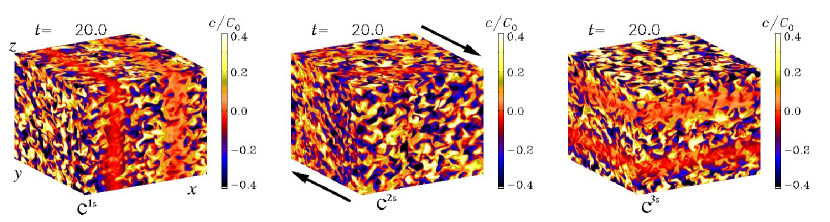
Figure 1: (Color online) Visualization of $c^{1s}$, $c^{2s}$, and $c^{3s}$ on the periphery of the computational domain after about one turnover time for a run with $k/k_{\rm f}=0.1$. In the middle panel, arrows indicate the direction of the shear flow with negative $S$, i.e. ${\rm d}{}\overline{U}_{y}/{\rm d}{}x<0$. Note the clear sinusoidal modulation in the $x$, $y$, and $z$ directions for the three panels, respectively. In the middle panel this modulation is already smeared out by the shear.

In the following we are interested in the fluxes of the passive scalar concentration, $\overline{\mbox{\boldmath${\cal F}$}}{}=\overline{\mathchoice{\mbox{\boldmath$\displaystyle u$}}{\mbox{\boldmath$\textstyle u$}}{\mbox{\boldmath$\scriptstyle u$}}{\mbox{\boldmath$\scriptscriptstyle u$}}{}c}$, where $c=C-\overline{C}$ is the fluctuation around the mean concentration and $\mathchoice{\mbox{\boldmath$\displaystyle u$}}{\mbox{\boldmath$\textstyle u$}}{\mbox{\boldmath$\scriptstyle u$}}{\mbox{\boldmath$\scriptscriptstyle u$}}{}=\mathchoice{\mbox{\boldmath$\displaystyle U$}}{\mbox{\boldmath$\textstyle U$}}{\mbox{\boldmath$\scriptstyle U$}}{\mbox{\boldmath$\scriptscriptstyle U$}}{}-\overline{\bm{U}}$ is the velocity fluctuation around the mean flow $\overline{\bm{U}}$. The test-scalar equation is obtained by subtracting the averaged passive scalar equation from the original one and applying it to a predetermined set of six different mean fields,

$$\overline{C}^{ic}=C_{0}\cos kx_{i},\quad\overline{C}^{is}=C_{0}\sin kx_{i},\\$$ (28)

where $C_{0}$ is a normalization factor. Again, the overbars denote planar averaging over the directions that are perpendicular to the direction in which the mean field varies. For each test field $\overline{C}^{pq}$ we obtain a separate evolution equation for the corresponding fluctuating component $c^{pq}$,

$${\partial c^{pq}\over\partial t}=-\mathchoice{\mbox{\boldmath$\displaystyle\nabla$}}{\mbox{\boldmath$\textstyle\nabla$}}{\mbox{\boldmath$\scriptstyle\nabla$}}{\mbox{\boldmath$\scriptscriptstyle\nabla$}}{}\cdot(\overline{\bm{U}}c^{pq}+\mathchoice{\mbox{\boldmath$\displaystyle u$}}{\mbox{\boldmath$\textstyle u$}}{\mbox{\boldmath$\scriptstyle u$}}{\mbox{\boldmath$\scriptscriptstyle u$}}{}\overline{C}^{pq}+\mathchoice{\mbox{\boldmath$\displaystyle u$}}{\mbox{\boldmath$\textstyle u$}}{\mbox{\boldmath$\scriptstyle u$}}{\mbox{\boldmath$\scriptscriptstyle u$}}{}c^{pq}-\overline{\mathchoice{\mbox{\boldmath$\displaystyle u$}}{\mbox{\boldmath$\textstyle u$}}{\mbox{\boldmath$\scriptstyle u$}}{\mbox{\boldmath$\scriptscriptstyle u$}}{}c^{pq}})+\kappa\nabla^{2}c^{pq},$$ (29)

where $p=1$, …, 3, and $q=c$ or $s$. In this way, we calculate six different fluxes, $\overline{\mbox{\boldmath${\cal F}$}}{}^{pq}=\overline{\mathchoice{\mbox{\boldmath$\displaystyle u$}}{\mbox{\boldmath$\textstyle u$}}{\mbox{\boldmath$\scriptstyle u$}}{\mbox{\boldmath$\scriptscriptstyle u$}}{}c^{pq}}$, and compute the nine relevant components of $\kappa_{ij}$,

$$\kappa_{ij}=-\langle\cos kx_{j}\overline{\cal F}_{i}^{js}-\sin kx_{j}\overline{\cal F}_{i}^{jc}\rangle/k,$$ (30)

for $i,j=1,...,3$. Here, angular brackets denote volume averages. A visualization of $c^{1s}$, $c^{2s}$, and $c^{3s}$ on the periphery of the computational domain is shown in Fig. 1 after about one turnover time for a run with $k/k_{\rm f}=0.1$, which is smaller than in most of the runs analyzed in this paper. This ratio is chosen here for visualization purposes only, because this way the large-scale modulation compared with the scale of the turbulence becomes evident.

We emphasize that Eq. (29) is an inhomogeneous equation in $c^{pq}$. The term $\mathchoice{\mbox{\boldmath$\displaystyle u$}}{\mbox{\boldmath$\textstyle u$}}{\mbox{\boldmath$\scriptstyle u$}}{\mbox{\boldmath$\scriptscriptstyle u$}}{}\overline{C}^{pq}$ can be regarded as a forcing term that guarantees that the direction of the turbulent concentration flux will not change with time.

In this paper we present the values of $\kappa_{ij}$ in non-dimensional form by normalizing with

$$\kappa_{\rm t0}=u_{\rm rms}/3k_{\rm f},$$ (31)

which is the expected value for large values of Pe. Here we have defined the root-mean-square value of the velocity fluctuation as $u_{\rm rms}=\langle\mathchoice{\mbox{\boldmath$\displaystyle u$}}{\mbox{\boldmath$\textstyle u$}}{\mbox{\boldmath$\scriptstyle u$}}{\mbox{\boldmath$\scriptscriptstyle u$}}{}^{2}\rangle^{1/2}$.

Our simulations are characterized by two important non-dimensional control parameters, the shear parameter Sh and the Peclet number Pe, defined as

$$\mbox{\rm Sh}=S/(u_{\rm rms}k_{\rm f}),\quad\mbox{\rm Pe}=u_{\rm rms}/(\kappa k_{\rm f}).$$ (32)

In addition, there is the Schmidt number $\mbox{\rm Sc}=\nu/\kappa$, but we keep it equal to unity in all cases reported below. Note also that in most cases we use negative values of $S$, so we have $\mbox{\rm Sh}<0$. The smallest wave number that fits into the computational domain is $k_{1}=2\pi/L$. In most of the cases reported below we choose the forcing wave number to be 3 times larger, i.e. $k_{\rm f}/k_{1}=3$.

The simulations have been carried out using the Pencil Code which is a high-order finite-difference code (sixth order in space and third order in time) for solving the compressible hydrodynamic equations. The test-scalar equations where already implemented into the public-domain code, but have now been generalized to determining all nine components of $\kappa_{ij}$. The numerical resolution used in the simulations depends on the Peclet number and reaches $128^{3}$ meshpoints for runs with $\mbox{\rm Pe}\approx 120$. In this paper we restrict ourselves to time spans short enough so that the so-called vorticity dynamo has no time do develop; see Refs. EKR03 ; KMB09 for details on this effect.

III Results

III.1 Dependence on the shear parameter

We begin by discussing the dependence of the coefficients in Eq. (6) on the shear parameter Sh. The result is shown in Fig. 2 for $\mbox{\rm Pe}=25$. It turns out that all five coefficients are positive. We find that $\kappa_{\rm t}/\kappa_{\rm t0}={\rm const}{}=2$ for non-helical turbulence and 3 for helical turbulence, independent of the value of shear, provided $|\mbox{\rm Sh}|<0.5$. The other coefficients show the following approximate scaling behavior:

$$\kappa_{\sf S}S/\kappa_{\rm t0}\approx 5|\mbox{\rm Sh}|,\quad\kappa_{{\sf S}{\sf S}}S^{2}\!/2\kappa_{\rm t0}\approx 30\,\mbox{\rm Sh}^{2},$$ (33)

$$\kappa_{\sf A}S/\kappa_{\rm t0}\approx 10\,|\mbox{\rm Sh}|^{3},\quad\kappa_{{\sf A}{\sf S}}S^{2}/2\kappa_{\rm t0}\approx 40\,|\mbox{\rm Sh}|^{3}.$$ (34)

The fact that $\kappa_{\sf A}$ and $\kappa_{{\sf A}{\sf S}}$ scale with the third power of Sh suggests that these are higher order effects that are not easily captured by perturbative approaches.

Figure 2: Dependence of the coefficients in Eq. (6) on Sh for $\mbox{\rm Pe}=25$. The dashed line in the first panel is for a run with maximum helicity. All runs with helicity are marked with open symbols. Filled symbols indicate runs without helicity. Solid lines represent the fits given by Eqs. (33) and (34).

A comment regarding the values of Sh is here in order. Although values of Sh larger than unity have not yet been explored, it is unlikely that the uprise of $\kappa_{\rm t}$ continues. Furthermore, one might speculate that all coefficients in Eqs. (33) and (34) should eventually decrease as $|\mbox{\rm Sh}|\to\infty$.

In Fig. 2 we have also shown results for cases where the forcing function has maximum helicity. No significant dependence can be seen, except for $\kappa_{\rm t}$ which is slightly enhanced in the helical case with weak shear. This suggests that this dependence is not connected with the presence of shear.

III.2 Dependence on Peclet number

We have performed simulations for different values of the Peclet number and have determined the coefficients in Eq. (6) for each simulation. The results are shown in Fig. 3 for fixed $\mbox{\rm Sh}=0.2$. It turns out that the first four coefficients can well be approximated by simple algebraic functions,

$${\kappa_{\rm t}\over\kappa_{\rm t0}}={2\kappa_{\rm Sh}\mbox{\rm Pe}^{2}\over\mbox{\rm Pe}_{0}^{2}+\mbox{\rm Pe}^{2}},\quad{\kappa_{\sf S}S\over\kappa_{\rm t0}}={\kappa_{\rm Sh}\mbox{\rm Pe}^{3}\over(\mbox{\rm Pe}_{0}^{2}+\mbox{\rm Pe}^{2})^{3/2}},$$ (35)

$${\kappa_{{\sf S}{\sf S}}S^{2}\over 2\kappa_{\rm t0}}={\kappa_{\rm Sh}\mbox{\rm Pe}^{4}\over(\mbox{\rm Pe}_{0}^{2}+\mbox{\rm Pe}^{2})^{2}},\quad{\kappa_{\sf A}S\over\kappa_{\rm t0}}={\kappa_{\rm Sh}\mbox{\rm Pe}^{4}\over(\mbox{\rm Pe}_{0}^{2}+\mbox{\rm Pe}^{2})^{2.4}},$$ (36)

where $\kappa_{\rm Sh}=0.95\kappa_{\rm t0}$ and $\mbox{\rm Pe}_{0}=3.8$ are fit parameters. In the case of $\kappa_{{\sf A}{\sf S}}$ the error bars are so large that no conclusive statements can be made. Likewise, the error bar on the first data point is quite large too. This is caused by the numerical time step becoming rather short at large diffusivities, so the run is short and the statistics poor.

Figure 3: Dependence of the coefficients in Eq. (6) on Pe for $\mbox{\rm Sh}=-0.2$. The symbols give the numerical results and the solid lines represent fits given by Eqs. (35) and (36).

In Fig. 4 we show the dependence of the diagonal components of $\kappa_{ij}$ on Pe. Over the range of parameters shown here, the difference between the three components is small, although there is a tendency for $\kappa_{yy}$ to be somewhat enhanced around $\mbox{\rm Pe}=20$, while $\kappa_{zz}$ is slightly smaller than $\kappa_{xx}$.

Figure 4: Dependence of the diagonal components of $\kappa_{ij}$ on Pe.

III.3 Wavenumber dependence

We consider now the dependence of the diagonal components of $\kappa_{ij}$ on the wave number $k$ of the test scalar in Eq. (28). A dependence of $\kappa_{ij}$ on $k$ reflects the fact that there is poor scale separation, i.e. $k/k_{\rm f}$ is no longer small. In such a case, the multiplication with a turbulent diffusivity in Eqs. (1) and (2) must be replaced by a convolution with an integral kernel BSV09 . In Fourier space the convolution corresponds to a multiplication. The full integral kernel can be assembled by determining the full $k$ dependence and then Fourier transforming back into real space.

Figure 5: Dependence of the diagonal components of $\kappa_{ij}$ on $k$ for $\mbox{\rm Sh}=-0.13$ at $\mbox{\rm Pe}=40$ (upper panel) and $\mbox{\rm Sh}=-0.20$ at $\mbox{\rm Pe}=60$ (lower panel).

The resulting dependence on $k$ is shown in Fig. 5 for two values of the shear parameter and Pe around 50. In agreement with earlier findings, the components of $\kappa_{ij}$ show a Lorentzian dependence on $k$, i.e.

$$\kappa_{ij}={\kappa_{ij}^{(0)}\over 1+(ak/k_{\rm f})^{2}},$$ (37)

where $a\approx 0.2$ for the $\kappa_{11}$ and $\kappa_{22}$ components, and $a\approx 0.4$ for the $\kappa_{33}$ component. Here, $\kappa_{ij}^{(0)}$ is the value for $k=0$, which is approximately equal to $\kappa_{\rm t0}$, defined in Eq. (31).

Given that the Schmidt number is always kept equal to unity, there will be a fully developed cascade in the passive scalar concentration when the Peclet number is large. The validity of Eq. (37) has only been tested for values of Pe up to 60. It is unclear whether this equation holds also for large values of Pe when contributions from the high wave number dynamics may become important in the mixing of the mean concentration.

The case of high wave numbers is interesting in view of possible applications of our results to subgrid scale modeling in large-eddy simulations of turbulence. The highest possible wave number is the Nyquist wave number, $k_{\rm Ny}=\pi/\delta x$, where $\delta x$ is the mesh scale. In the Smagorinsky model Sma63 the subgrid scale viscosity is proportional to the modulus of the rate of strain tensor times $\delta x^{2}$. For a turbulent flow where the local velocity difference $\delta u_{\ell}$ over a distance $\ell$ is proportional to $\ell^{1/3}$ we expect the subgrid scale viscosity to be effectively proportional to $\ell^{4/3}$, suggesting an asymptotic $k^{-4/3}$ scaling for $k\gg k_{\rm f}$. Here we have identified $\ell$ with $\delta x$ and thus $k$ with $k_{\rm Ny}$. Only for a smooth velocity field, where $\delta u_{\ell}$ scales linearly with the separation $\ell$, the subgrid scale viscosity would be proportional to $\ell^{2}$, justifying an asymptotic $k^{-2}$ scaling. This uncertainty warrants further studies of the validity of Eq. (37) for $k\gg k_{\rm f}$.

III.4 Effects of helicity

As discussed in the Introduction, the presence of helicity allows one in principle to construct proper tensors proportional to $\overline{W}_{i}\overline{U}_{j}$ and $\overline{W}_{j}\overline{U}_{i}$, because we have now access to a pseudoscalar given by the kinetic helicity of the turbulence. If this does indeed have an effect, one would expect finite $yz$ and $zy$ components. In Fig. 6 we present results for $\kappa_{yz}$ and $\kappa_{zy}$ using $\mbox{\rm Pe}=25$. We see that $\kappa_{yz}=\kappa_{zy}=0$ within error bars, so there is no evidence for the presence of additional terms when the turbulence is helical.

Figure 6: Plot of $\kappa_{yz}$ (dotted line) and $\kappa_{zy}$ (dashed line) versus Sh for maximally helical turbulence and $\mbox{\rm Pe}=25$. No significant dependence can be seen.

IV Expectations from the $\tau$ approximation

Passive scalar transport is closely related to the transport of a mean magnetic field. Commonly applied techniques for computing turbulent transport coefficients in mean-field electrodynamics are the first order smoothing approximation Mof78 ; KR80 and the $\tau$ approximation VK83 ; KMR96 ; RKR03 . The $\tau$ approximation consists in writing down an evolution equation for the quadratic correlations which, in the case of mean-field electrodynamics, is the mean electromotive force $\overline{\mbox{\boldmath${\cal E}$}}{}$. Its solution gives then an expression for $\overline{\mbox{\boldmath${\cal E}$}}{}$ in terms of the mean magnetic field and its derivatives. For a recent review see Ref. BS05 . This technique has also been used to compute the Reynolds and Maxwell stress in rotating shear flows Ogi03 ; GO05 ; LiljeO09 . In the present case of passive scalar transport one starts with the evolution equation for the mean flux $\overline{\mbox{\boldmath${\cal F}$}}{}=\overline{\mathchoice{\mbox{\boldmath$\displaystyle u$}}{\mbox{\boldmath$\textstyle u$}}{\mbox{\boldmath$\scriptstyle u$}}{\mbox{\boldmath$\scriptscriptstyle u$}}{}c}$, as is done in Refs. BF03 ; BKM04 . Thus, we write

$${\partial\overline{\cal F}_{i}\over\partial t}=\overline{\dot{u}_{i}c}+\overline{u_{i}\dot{c}},$$ (38)

where dots denote time derivatives that are given essentially by Eqs. (24) and (29). This results in quadratic and triple correlations. The sum of all triple correlations is substituted by a damping term of the form $-\overline{\mbox{\boldmath${\cal F}$}}{}/\tau$ on the right-hand side of the evolution equation for $\overline{\mbox{\boldmath${\cal F}$}}{}$. Here, $\tau=\mbox{\rm St}/u_{\rm rms}k_{\rm f}$ is the turnover time and St is a positive dimensionless parameter of order unity (referred to as Strouhal number). This is a closure assumption that cannot be motivated rigorously RR07 , but it has been found numerically that the triple-correlations are indeed locally and temporally proportional to the negative flux term divided by $\tau$; see Ref. BKM04 for passive scalar diffusion and Ref. BS05b for the case of mean-field electrodynamics.

As a first orientation, and in order to gain some understanding of our numerical results, we make the additional assumption that we can subsume the effects of the pressure term in our closure assumption. Since our forcing function $\textstyle f$ is $\delta$ correlated in time we have $\overline{\mathchoice{\mbox{\boldmath$\displaystyle f$}}{\mbox{\boldmath$\textstyle f$}}{\mbox{\boldmath$\scriptstyle f$}}{\mbox{\boldmath$\scriptscriptstyle f$}}{}c}=\bm{0}$ and thus obtain

$$\overline{\dot{u}_{i}c}=-S\delta_{i2}\delta_{1k}\overline{u_{k}c}+\mbox{triple correlations},$$ (39)

$$\overline{u_{i}\dot{c}}=-\overline{u_{i}u_{j}}\,\nabla_{j}\overline{C}+\mbox{triple correlations}.$$ (40)

The triple correlation terms result from the nonlinearities in the evolution equations, Eqs. (24) and (29). In the $\tau$ approximation one substitutes the sum of the triple correlations by quadratic correlations, i.e. in the present case by $-\overline{u_{i}c}/\tau$ VK83 ; KRR90 . We write the resulting equation in matrix form,

$$\tau{\partial\overline{\cal F}_{i}\over\partial t}=-{\sf L}_{ik}\overline{\cal F}_{k}-\tau\overline{u_{i}u_{j}}\,\nabla_{j}\overline{C},$$ (41)

where ${\sf L}_{ik}=\delta_{ik}+S\tau\delta_{i2}\delta_{1k}$. We solve this equation for $\overline{\mbox{\boldmath${\cal F}$}}{}$ and obtain

$$\overline{\cal F}_{i}=-(\mbox{\boldmath${\sf L}$}{}^{-1})_{ij}\left(\tau\overline{u_{j}u_{k}}\,\nabla_{k}\overline{C}+\tau{\partial\overline{\cal F}_{i}\over\partial t}\right),$$ (42)

where $(\mbox{\boldmath${\sf L}$}{}^{-1})_{ik}=\delta_{ik}-\mbox{\rm Sh}\,\delta_{i2}\delta_{1k}$ with $\mbox{\rm Sh}=S\tau$. In the presence of shear, the Reynolds stress tensor $\overline{u_{j}u_{k}}$ is no longer diagonal, but it has finite $xy$ and $yx$ components. Also the three diagonal components are no longer the same. In the following we represent $\overline{u_{j}u_{k}}$ in the form

$$\overline{\mathchoice{\mbox{\boldmath$\displaystyle u$}}{\mbox{\boldmath$\textstyle u$}}{\mbox{\boldmath$\scriptstyle u$}}{\mbox{\boldmath$\scriptscriptstyle u$}}{}\mathchoice{\mbox{\boldmath$\displaystyle u$}}{\mbox{\boldmath$\textstyle u$}}{\mbox{\boldmath$\scriptstyle u$}}{\mbox{\boldmath$\scriptscriptstyle u$}}{}}=\overline{u_{x}^{2}}\pmatrix{1&-\delta&0\cr-\delta&1+\epsilon&0\cr 0&0&1+\epsilon_{z}},$$ (43)

where $\delta=-\overline{u_{x}u_{y}}/\overline{u_{x}^{2}}$ characterizes the value of the off-diagonal components, while $\epsilon=\overline{u_{y}^{2}}/\overline{u_{x}^{2}}-1$ and $\epsilon_{z}=\overline{u_{z}^{2}}/\overline{u_{x}^{2}}-1$ characterize the change in the two lower diagonal components. The dependence of $\delta$ and $\epsilon$ on Sh is shown in Fig. 7, while $\epsilon_{z}$ is found to be small. Inserting this expression into Eq. (42), we obtain

$${{\bm{\kappa}}\over\kappa_{\rm t0}}=\pmatrix{1&-\delta&0\cr-\delta-\mbox{\rm Sh}&1+\epsilon+\delta\mbox{\rm Sh}&0\cr 0&0&1+\epsilon_{z}}.$$ (44)

In the stationary state we may ignore the time derivative and recover Eq. (3) with

$${\kappa_{\sf S}S\over\kappa_{\rm t0}}=-2\delta-\mbox{\rm Sh},\quad{\kappa_{\sf A}S\over\kappa_{\rm t0}}=-\mbox{\rm Sh},$$ (45)

$${\kappa_{\sf SS}S^{2}\!/2\over\kappa_{\rm t0}}+2\epsilon_{z}={\kappa_{\sf AS}S^{2}\!/2\over\kappa_{\rm t0}}=\epsilon-\delta\mbox{\rm Sh}.$$ (46)

We recall that Sh is negative, and that $\delta$ changes sign with Sh. Therefore we expect $\kappa_{\sf S}$ and $\kappa_{\sf A}$ to be positive, which agrees with the simulations. Furthermore, we expect $\kappa_{yy}$ to be enhanced, which also agrees with the simulations. However, the slight suppression of $\kappa_{zz}$ cannot be explained by the simple theory, because $\epsilon_{z}$ is small and perhaps even positive, suggesting at best an opposite trend.

Figure 7: Dependence of $\delta$ and $\epsilon$ on Sh for nonhelical turbulence (solid symbols) and helical turbulence (open symbols). The solid line in the second panel has a slope of 5.

V Conclusions

The present work has shown that shear introduces anisotropies in the diffusivity tensor for passive scalar diffusion. These additional components are proportional to the even and odd parts of the velocity gradient tensor, as well as products of these tensors. Those components that are connected with the antisymmetric part of the velocity gradient tensor scale with the third power of the shear parameter, suggesting that these effects cannot be captured perturbatively.

Given that $\mbox{\rm Sc}=1$ in all our runs, we always have $\mbox{\rm Re}=\mbox{\rm Pe}$, which is at most about 100, so the inertial range of the turbulence is not very big yet. It is therefore important to investigate the dependence of the various transport coefficients on the values of Re and Pe, as was done in Fig. 3. The results available so far suggest that the first three coefficients ($\kappa_{\rm t}$, $\kappa_{\sf S}$, and $\kappa_{{\sf S}{\sf S}}$) do not change with Re for $\mbox{\rm Re}>10$. If there were indications that the resulting coefficients change beyond $\mbox{\rm Re}=100$, it would be important to make an effort to increase the values of Re even further. This would require more resolution and is obviously expensive. In view of the constancy of the first three coefficients, this may not be well justified. The fourth coefficient ($\kappa_{\sf A}$) seems to tend to zero, and the fifth one ($\kappa_{{\sf A}{\sf S}}$) shows large error bars. The situation regarding these last two coefficients may not improve significantly towards larger Reynolds numbers, unless the simulations are run for long enough time.

In general, turbulent transport tends to be enhanced in the direction of the shear, i.e. $\kappa_{yy}$ tends to be larger than $\kappa_{xx}$ and $\kappa_{zz}$. Furthermore, $\kappa_{zz}$ tends to be suppressed relative to $\kappa_{xx}$. This is a result that is not reproduced by a simple analytical closure in which triple correlations are being replaced with quadratic ones. In particular, there is no evidence for a suppression of turbulent transport in the cross-stream or $x$ direction. Instead, there is a suppression in the spanwise direction out of the plane of the shear flow.

We recall that the moduli of the diagonal components of the turbulent diffusivity tensor are found to decrease with increasing wave number of the mean concentration in a Lorentzian fashion. This is in agreement with earlier findings both in the contexts of mean-field electrodynamics with and without shear BRS08 ; Mitra_etal09 , as well as passive scalar transport in the absence of shear BSV09 . The limit of high wave numbers may be of interest for subgrid scale modeling in large-eddy simulations of turbulence. However, it still needs to be clarified whether the effective diffusivity is proportional to the inverse Nyquist wave number to the second power, as suggested by our current results, or to some smaller power, $\sim k^{-4/3}$, as expected for Kolmogorov turbulence. In order to address this question, simulations at larger Peclet and Reynolds numbers are required. Such simulations do not require the presence of shear. This is however beyond the scope of the present paper.

Finally, we note that, in shear flows, the passive scalar transport properties are not affected by the presence of helicity. In other words, there is no evidence for the existence of components to the turbulent diffusivity tensor $\kappa_{ij}$ that are proportional to $\overline{W}_{i}\overline{U}_{j}$ and $\overline{W}_{j}\overline{U}_{i}$.

$Header: /var/cvs/brandenb/tex/eniko/testscalar_shear/paper.tex,v 1.32 2010-07-02 19:11:29 brandenb Exp $