The initial conditions of stellar protocluster formation

Abstract

Context. The majority of stars form in clusters. Therefore a comprehensive view of star formation requires understanding the initial conditions for cluster formation.

Aims. The goal of our study is to shed light on the physical properties of infrared dark clouds (IRDCs) and the role they play in the formation of stellar clusters. This article, the first of a series dedicated to the study of IRDCs, describes techniques developed to establish a complete catalogue of Spitzer IRDCs in the Galaxy.

Methods. We have analysed Spitzer GLIMPSE and MIPSGAL data to identify a complete sample of IRDCs in the region of Galactic longitude and latitude $10^{\circ}<|l|<65^{\circ}$ and $|b|<1^{\circ}$. From the 8$\mu$m observations we have constructed opacity maps and used a newly developed extraction algorithm to identify structures above a column density of N${}_{\rm{H_{2}}}\ga 1\times 10^{22}$ cm^-2. The 24$\mu$m data are then used to characterize the star formation activity of each extracted cloud.

Results. A total of 11303 clouds have been extracted. A comparison with the existing MSX based catalogue of IRDCs shows that 80$\%$ of these Spitzer dark clouds were previously unknown. The algorithm also extracts $\sim$ 20000 to 50000 fragments within these clouds, depending on detection threshold used. A first look at the MIPSGAL data indicates that between 20% and 68% of these IRDCs show 24$\mu$m point-like association.This new database provides an important resource for future studies aiming to understand the initial conditions of star formation in the Galaxy.

1 Introduction

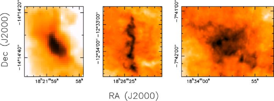
Figure 1: These images show the GLIMPSE Spitzer 8$\mu$m emission of 3 random IRDCs from our sample. These illustrate the diversity in shape and size of IRDCs.

The majority of stars form in groups from few tens to few hundreds of objects (e.g. Lada & Lada, 2003). So, understanding cluster formation is key to understanding the formation of stars. Clusters form from the gas located in the densest parts of molecular clouds, within structures called clumps (Blitz, 1993). These clumps fragment into an assembly of protostellar cores which collapse to produce stars, forming ‘protoclusters’. By definition, protoclusters are active star forming regions, with jets, flows and heating sources (e.g. Bally et al., 2006) which rapidly start to shape their surroundings. From the study of these protoclusters, it is therefore difficult to back track to the initial conditions of their formation. On the other hand, clumps which are on the verge of forming protostars, but which have not formed any yet, are structures unpolluted by star formation activity and must still reflect the initial conditions of the formation of protoclusters. Looking for, and studying such ‘pre-protoclusters’ is crucial for our understanding of star formation processes.

Only a tiny percentage of the material in any molecular cloud forms stars. These star-forming regions are traced by various signposts of star formation activity such as the presence of strong infrared sources, outflows, jets, methanol and water masers and compact HII regions. The problem with identifying pre-protoclusters is that by definition these signposts are not yet present. Other means are thus necessary to find such objects. The two infrared satellites ISO and MSX have been important tools for this purpose. Indeed, the large infrared surveys these satellites carried out identified infrared dark structures, seen in absorption from 7 to 25 $\mu$m against the background emission (Perault et al., 1996; Hennebelle et al., 2001; Egan et al., 1998; Simon et al., 2006a) . Millimeter molecular lines (e.g. Carey et al., 1998; Teyssier et al., 2002; Pillai et al., 2006) and dust continuum observations (e.g. Teyssier et al., 2002; Rathborne et al., 2006) have clearly demonstrated that these infrared dark clouds are dense, cold structures, possibly being the progenitors of protoclusters (Simon et al., 2006b). Rathborne et al. (2006) even suggested that the dust continuum “cores” observed in these IRDCs are the direct progenitors of massive stars. However, the wide range of mass and size of these IRDCs clearly suggests that they cannot all be evolving along the same evolutionary path and they must lead to the formation of a large range of different stellar contents.

So far, the study of the earliest stages of the formation of protoclusters have mostly focussed on the closest objects such as $\rho$-Oph(e.g. Motte et al., 1998; André et al., 2007), Perseus (Hatchell et al., 2005; Enoch et al., 2006), NGC2264 (e.g. Peretto et al., 2006; Teixeira et al., 2006). The results of these studies set important constraints on models of star formation, but may not be representative of the formation of stars throughout the Galaxy. The only way to define such a representative view is through studies of large unbiased samples of the precursors of stellar clusters.

In this paper we identify and characterise the IRDCs detected using the Spitzer GLIMPSE and MIPSGAL archive data. The high angular resolution of the Spitzer data provides a detailed probe of the structure of these sources while the high sensitivity of IRAC and MIPS allows us to detect previously unseen deeply embedded protostars/protoclusters. Section 2 of this paper presents the Spitzer archive data used for this study. Section 3 will discuss the construction of 8$\mu$m opacity maps for IRDCs, while Section 4 will focus on the conversion from 8$\mu$m opacity to H₂ column density. The extraction of structures within these maps will be discussed in Section 5. A comparison with the MSX catalogue of IRDCs is in Section 6 while Section 7 summarizes our initial study. The nature of these dark clouds and their star formation actively are discussed in more detail in subsequent papers (Peretto & Fuller, in preparation).

2 A large survey of infrared dark clouds: Spitzer archive data

IRDCs are seen in silhouette against the infrared background emission (see Fig. 1) and as a sample are likely to contain protoclusters and pre-protoclusters. Even when large scale (sub)millimetre surveys of the Galactic plane become available and these objects can be detected through their dust emission, IRDCs and studies of the absorption towards these sources will remain important. Not only can the IRDCs be studied at high angular resolution at infrared wavelengths, but unlike the (sub)millimetre emission, their column density can be measured from the absorption independent of the dust temperature.

The first large survey of IRDCs was undertaken by Simon et al. (2006a) using the mid-infrared data of the MSX satellite. In total, Simon et al. detected more than 10000 IRDCs, with sizes larger than (36^′′)² and flux density more than 2 MJy/sr ($>2$ times the rms noise of the MSX images) below the mid-infrared radiation field. Within these IRDCs they extracted more than 12000 IRDC “cores”. Simon et al. (2006b) performed a follow up of a sub-sample of few hundreds sources for which they were able to determine distances. They found that these IRDCs are very similar to CO molecular clumps (e.g. Blitz, 1993).

In the GLIMPSE and MIPSGAL surveys the Spitzer satellite has resurveyed a large fraction of the Galactic plane at infrared wavelengths ($10\hbox{${}^{\circ}$}<|l|<65\hbox{${}^{\circ}$},0<|b|<1\hbox{${}^{\circ}$}$). These data have both better angular resolution (2^′′  vs 20^′′ at 8$\mu$m ) and sensitivity (0.3 MJy/sr vs 1.2 MJy/sr at 8$\mu$m ) than the MSX data, as well as wider wavelength coverage.The IRAC (3.6, 4.5, 5.8, 8 $\mu$m) GLIMPSE and MIPS (24, 70, 160 $\mu$m) MIPSGAL observations provide a unique opportunity to shed light on the role of IRDCs during the earliest stages of star formation. Despite a smaller coverage of the Galactic plane by Spitzer, an initial comparison of the MSX IRDC catalogues with the Spitzer observations indicated that the Spitzer data contained IRDCs undetected by MSX in the same region of the Galaxy. Therefore an unbiased search of the Spitzer GLIMPSE data has been undertaken to identify IRDCs.

Many IRDCs can been seen in silhouette up to at least 24 $\mu$m, providing a wide wavelength range over which they can be studied in absorption. However several factors affect the choice of the optimal wavelength at which to identify and study the overall cloud properties. These include the strength and uniformity of the background emission and the number of foreground and background stars and in principle, the wavelength dependence of the dust extinction law, although recent work suggests that from 4.5 to 8$\mu$m, the three last bands observed by Spitzer/IRAC, the extinction is a relatively flat function of wavelength (Lutz et al., 1996; Indebetouw et al., 2005; Román-Zúñiga et al., 2007). The angular resolution of the observations is highest at the shortest wavelengths, but in these bands a very high density of stars is detected and high degree of structure in the relatively weak background emission makes analysis of the images at these wavelengths complex. Overall, inspection of the Spitzer data shows that the strength and relative smoothness of the background emission together with the relatively low density of stars make the IRAC 8 $\mu$m band the most suitable for this initial study of a large sample of objects.

The GLIMPSE and MIPSGAL data have been reduced and calibrated automatically to produce the so called post-Basic Calibrated Data (post BCD). The typical flux uncertainty for point-like sources is $\sim 2\%$ at 8$\mu$m (Reach et al., 2005) while the position uncertainty is less than 0.3^′′(IRAC manual V8.0: http://ssc.spitzer.caltech.edu/documents/SOM/). However, because we are not looking at point-like sources but extended objects, a calibration factor has to be applied on the PBCD 8$\mu$m images (Reach et al., 2005). This calibration factor, CF, is a function of the aperture radius, R_a, for the source under investigation (http://ssc.spitzer.caltech.edu/irac/calib/extcal/). The relation between CF and R_a in arcseconds, at 8$\mu$m is $CF=1.37\times\exp(-R_{a}^{0.33})+0.74$. Because the typical size of the structure we analyse is about one arcminute, in the analysis which follows we applied a calibration factor of 0.8 to the PBCD 8$\mu$m images. A different calibration factor would not change the opacities of the IRDCs we calculated, but would imply different related intensities (Table 1).

Figure 2: Schematic view a typical IRDC flux density profile. The variable meanings used in the rest of the text are illustrated on this figure. In this figure, $I_{\rm{fore}}$ has been set to a particular value, e.g., 38 MJy/sr, but in practice, it can be anywhere between $I_{\rm{zl}}$ and $I_{\rm{min}}$.

3 Opacity distribution of IRDCs

3.1 Principle

Infrared dark clouds are structures seen in absorption against the background emission. The strength of the absorption is directly related to the opacity along the line of sight. Following the notation of Bacmann et al. (2000), the relation between the opacity $\tau_{\lambda}$ and the intensity at wavelength at $\lambda$, emerging from the cloud $I_{\lambda}$, is given by

$$I_{8\mu\rm{m}}=I_{\rm{bg}-8\mu\rm{m}}\times\exp(-\tau_{8\mu\rm{m}})+I_{\rm{fore}-8\mu\rm{m}}$$ (1)

where $I_{\rm{bg}-8\mu\rm{m}}$ is the intensity of the background emission at 8$\mu$m, and $I_{\rm{fore}-8\mu\rm{m}}$ is the foreground emission. In the following for simplicity we drop the 8$\mu$m label on the variable names, except on the opacity. If we know the foreground and background intensities we can invert Eq. (1) and infer the spatial distribution of the opacity within an infrared dark cloud,

$$\tau_{8\mu\rm{m}}=-\ln\left(\frac{I-I_{\rm{fore}}}{I_{\rm{bg}}}\right)$$ (2)

$I_{\rm{fore}}$ and $I_{\rm{bg}}$ are related to each other by $I_{\rm{MIR}}=I_{\rm{bg}}+I_{\rm{fore}}$ where $I_{\rm{MIR}}$ is the observed mid-infrared radiation field and can be estimated directly from the $8\mu$m images (see Fig. 2). A lower limit on $I_{\rm{fore}}$ is given by the intensity of the zodiacal light, $I_{\rm{zl}}$, in the direction of the cloud, while an upper limit is given by the minimum intensity within the cloud, $I_{\rm{min}}$. However, with the extinction data only, it is impossible to find the exact value of $I_{\rm{fore}}$ for a given cloud.

The determination of $I_{\rm{fore}}$ is crucial to infer the spatial opacity distribution of a given IRDC. To illustrate this point, we computed the opacity of the cloud profile shown in Fig. 2 for three different values of $I_{\rm{fore}}$ (Fig. 3). On this figure we see that, with increasing $I_{\rm{fore}}$, the opacity increases significantly everywhere in the cloud, and even more sharply at the peak. These opacity variations are even more drastic for shallower clouds. It is therefore important to constrain $I_{\rm{fore}}$ when calculating the opacity distribution of an IRDC.

Figure 3: Calculated opacity profiles of the IRDC plotted in Fig.2 corresponding to 3 different assumptions on the foreground intensity. The solid line shows $I_{\rm{fore}}=I_{\rm{zl}}$ (i.e $I_{\rm{fore}}=0.25\times I_{\rm{min}}$), the dotted line $I_{\rm{fore}}=0.7\times I_{\rm{min}}$ and the dashed line $I_{\rm{fore}}=0.9\times I_{\rm{min}}$ .

Of course it is also possible that at least some the IRDCs are saturated and their intensity profiles become flattened. In such cases, it becomes impossible to recover the central structure of the clouds through the extinction maps. Moreover, such flattening could lead to an incorrect interpretation of the final opacity profiles of IRDCs.

Table 1: SDC properties for the first 30 out of 11303 in the catalogue. The full catalogue is available online. The columns give a running number (1), the name of the source based in its Galactic coordinates (2), the right ascension and declination (in J2000) of the cloud peak (3,4), the minimum 8$\mu$m emission towards the cloud ($I_{\rm{min}}$) (5), the background 8$\mu$m emission ($I_{\rm{MIR}}$) (6), the maximum $I_{\rm{MIR}}$ variation within the IRDC ($\delta I_{\rm{MIR}}$, Sec. 3.3) (7), the size of the cloud along its major and minor axes in arcseconds (8,9), the position angle of the major axis of the cloud in degrees East of North (10), the equivalent radius ($R_{\rm{eq}}$; Sec. 5.1) of the cloud (11), the peak and average optical depth of the cloud at 8$\mu$m (12,13), the optical depth at 8$\mu$m at which the absorption would be saturated (14), the number of fragments in the cloud identified with $\tau_{\rm{step}}=0.35$ (15; Sec. 5.2), whether there are 24$\mu$m stars in the field (16) and in the cloud (17; Sec. 5.3); and the density of stars around the cloud (18).

Number	Name	Coordinates		$I_{\rm{min}}$	$I_{\rm{MIR}}$	$\delta I_{\rm{MIR}}$	$\Delta X$	$\Delta Y$	$\alpha$	Req	$\tau_{\rm{peak}}$	$\tau_{\rm{av}}$	$\tau_{\rm{sat}}$	frag	star		$\sigma_{\rm{star}}$
		RA(J2000)	Dec(J2000)	(MJy/sr)	(MJy/sr)		(′′)	(′′)	(∘)	(′′)					Field	IRDC	(arcmin-2)
1	SDC9.22+0.169	18:05:30.40	-20:53:16.0	37.9	55.7	0.07	42.9	29.8	76	32.3	1.16	0.50	4.45	2	y	y	0.92
2	SDC9.25+0.144	18:05:39.69	-20:52:25.6	40.8	56.9	0.04	26.9	20.5	-66	23.9	0.95	0.48	4.47	1	y	n	0.95
3	SDC9.256+0.133	18:05:42.92	-20:52:27.8	41.7	56.7	0.01	13.5	10.8	-42	13.1	0.85	0.48	4.47	1	n	n	1.33
4	SDC9.301+0.126	18:05:50.01	-20:50:16.8	43.0	56.7	0.00	17.9	7.2	-89	12.6	0.75	0.45	4.47	1	n	n	1.34
5	SDC9.328+0.031	18:06:14.76	-20:51:39.7	46.2	60.8	0.02	11.4	10.0	87	11.6	0.74	0.47	4.53	1	y	n	1.14
6	SDC9.403+0.26	18:05:33.02	-20:41:00.7	33.7	44.5	0.02	11.2	7.3	-87	10.2	0.75	0.44	4.22	1	y	n	0.93
7	SDC9.432+0.163	18:05:58.31	-20:42:21.8	38.7	51.4	0.03	13.3	8.4	-50	11.8	0.76	0.44	4.37	1	n	n	1.02
8	SDC9.461+0.138	18:06:07.50	-20:41:32.8	40.0	53.0	0.03	17.8	6.9	22	12.0	0.77	0.42	4.40	1	n	n	1.08
9	SDC9.624+0.187	18:06:16.80	-20:31:35.6	37.7	53.5	1.58	321.6	203.8	-75	188.7	4.30	0.61	4.41	6	y	y	0.78
10	SDC9.629-0.061	18:07:13.25	-20:38:38.7	38.0	51.7	0.03	23.0	16.1	30	18.0	0.85	0.45	4.37	1	y	n	0.94
11	SDC9.635+0.296	18:05:53.87	-20:27:49.8	24.1	39.7	0.08	29.6	15.1	-60	21.5	1.96	0.58	4.11	1	y	n	0.76
12	SDC9.689+0.000	18:07:06.92	-20:33:41.5	39.6	52.9	0.01	24.6	11.8	57	15.9	0.79	0.46	4.40	1	n	n	1.01
13	SDC9.692-0.55	18:09:10.79	-20:49:34.6	27.2	35.3	0.02	18.6	6.8	-69	12.7	0.69	0.41	3.99	1	n	n	0.94
14	SDC9.737-0.239	18:08:06.57	-20:38:08.1	37.9	52.1	0.05	30.4	12.4	4	20.3	0.91	0.48	4.38	1	n	n	0.97
15	SDC9.762-0.567	18:09:23.29	-20:46:20.9	26.6	37.3	0.01	12.1	7.5	-48	10.7	0.98	0.51	4.05	1	y	y	0.79
16	SDC9.787-0.156	18:07:54.17	-20:33:06.8	40.1	61.2	0.06	58.7	26.3	-26	37.1	1.38	0.57	4.54	2	y	n	1.13
17	SDC9.796-0.028	18:07:26.89	-20:28:53.3	43.5	59.8	0.04	36.6	17.7	-1	25.7	0.92	0.50	4.52	1	n	n	1.25
18	SDC9.798-0.707	18:09:59.42	-20:48:32.9	29.1	40.5	0.36	63.7	45.8	2	47.5	0.90	0.47	4.13	1	y	n	0.72
19	SDC9.819-0.141	18:07:54.93	-20:31:00.7	44.8	62.2	0.02	39.0	12.5	37	20.1	0.95	0.44	4.56	1	y	n	1.25
20	SDC9.825-0.03	18:07:30.72	-20:27:26.0	41.0	58.3	0.08	78.9	19.9	78	32.7	1.02	0.47	4.49	2	y	n	1.16
21	SDC9.844+0.752	18:04:38.31	-20:03:31.4	23.1	30.8	0.05	24.1	13.6	-52	16.8	0.76	0.43	3.86	1	y	n	0.56
22	SDC9.845-0.138	18:07:57.47	-20:29:34.3	37.0	63.5	0.05	67.9	35.1	0	37.5	2.28	0.51	4.58	2	y	n	1.16
23	SDC9.852-0.034	18:07:35.07	-20:26:07.8	30.5	59.3	0.17	119.4	55.6	-73	76.5	4.95	0.87	4.51	12	y	y	1.19
24	SDC9.859-0.746	18:10:15.75	-20:46:27.5	33.1	61.3	1.94	294.5	150.3	-7	162.8	3.08	0.79	4.54	4	y	y	0.63
25	SDC9.864-0.102	18:07:51.78	-20:27:30.2	49.1	64.5	0.02	35.2	17.3	84	23.4	0.74	0.44	4.59	1	y	n	1.18
26	SDC9.872-0.767	18:10:22.02	-20:46:23.9	42.5	69.3	1.51	180.5	113.6	-66	126.3	2.29	0.79	4.67	2	y	y	0.55
27	SDC9.878-0.11	18:07:55.37	-20:26:58.8	35.5	65.7	0.07	59.2	40.9	26	49.3	4.98	0.83	4.61	4	y	y	1.18
28	SDC9.889-0.747	18:10:19.58	-20:44:56.8	61.7	99.2	0.20	26.5	23.2	-16	24.8	2.01	0.92	5.02	1	y	n	0.59
29	SDC9.895-0.749	18:10:20.74	-20:44:41.4	73.5	105.0	0.04	12.6	6.4	18	9.9	1.07	0.54	5.08	1	n	n	0.57
30	SDC9.904-0.699	18:10:10.70	-20:42:43.9	58.7	78.9	0.38	39.5	19.2	43	26.9	0.73	0.47	4.80	1	y	n	0.49

3.2 Constraining $I_{\rm{fore}}$

Comparison of the infrared extinction and millimeter emission can be used to constrain the infrared foreground emission towards an IRDC by requiring that both techniques give the same column density towards the source. For this purpose we have used the 38 IRDC 1.2mm dust continuum images Rathborne et al. (2006) obtained with the IRAM 30m telescope at 11^′′angular resolution. The 1.2mm emission can be translated into an 8$\mu$m opacity, $\tau_{\rm{em}}$, using the equation

$$\tau_{\rm{em}}=\frac{S_{\rm{peak}}\times R_{\kappa}}{B_{1.2}(T_{d})\times\Omega_{\rm{30m}}}$$ (3)

where S_peak is the 1.2mm dust continuum emission peak of the source, $R_{\kappa}$ is the specific dust opacity ratio between 8$\mu$m and 1.2mm, $B_{1.2}(T_{d})$ is the Planck function at 1.2mm for the dust temperature $T_{d}$, and $\Omega_{30m}$ is the solid angle at 1.2mm of the IRAM 30m telescope beam. The value for $R_{\kappa}$ is not well constrained: different models of dusts provide different values of $R_{\kappa}$. Given the chemical composition of the emitting/absorbing dust the value of $R_{\kappa}$ can be as large as 2000 for interstellar dust in diffuse clouds (e.g. Draine, 2003), decreasing to 750 for dense clouds (e.g. Ossenkopf & Henning, 1994; Johnstone et al., 2003). Given the dense and cold nature of IRDCs, we adopted the value $R_{\kappa}=750$, and a dust temperature of 15 K, which gives

$$\tau_{\rm{em}}=0.02\times S_{\rm{peak}}$$ (4)

with $S_{\rm{peak}}$ in mJy/beam. After smoothing the Spitzer 8$\mu$m  images of the 38 IRDCs observed by Rathborne et al. (2006) to the same resolution as the the IRAM 30m 1.2mm images, we have constructed their 8$\mu$m  opacity maps assuming $I_{\rm{fore}}=I_{\rm{zl}}$ (i.e. the lower limit on the foreground emission). A direct comparison between these opacity maps and the ones calculated from the 1.2mm dust continuum images becomes then possible. However the observations of the 8$\mu$m absorption and 1.2mm emission are not equally sensitive to all of the dust along the line of sight. Regions of low column density are more easily detected in absorption than in emission. For this reason, we selected only clear corresponding peaks in both type of images, ending up with 57 “cores” (emission peaks and absorption minima) which have been used for the comparison. Amongst these cores 11 show 24$\mu$m point-like emission. Figure 4 shows the resulting comparison for these 57 cores, the “starless” ones (those without associated 24$\mu$m  emission) are marked with open triangles while the “protostellar” ones are marked with red stars. Also shown are the three lines: $\tau_{\rm{abs}}=\tau_{\rm{em}}$ (solid line), $\tau_{\rm{abs}}=2\times\tau_{\rm{em}}$, and $\tau_{\rm{abs}}=0.5\times\tau_{\rm{em}}$ (dashed lines). In the figure there is a clear separation between the starless sources and those objects associated with a 24$\mu$m point-like source. For the sources associated with 24$\mu$m point-like emission, the values of $\tau_{\rm{em}}$ are on average higher than for the starless sources. The $\tau_{\rm{em}}/\tau_{\rm{abs}}$ ratio is on average $\sim 2.9$ for the starless sources with a dispersion of 1.1, while it is $\sim 7.2$ for the sources with stars with a dispersion of 3.8. This reflects that the latter group of sources have stronger 1.2mm emission (a factor of $\sim 2.5$ ), which translates to higher opacities for the same assumed dust temperature. This clearly shows these sources are in fact either warmer with average dust temperature greater than 15 K, or else have different dust properties. On the other hand for the starless objects, the average ratio $<\tau_{\rm{em}}/\tau_{\rm{abs}}>=2.9$ is closer, but still rather far from, unity. This suggests that the value of $I_{\rm{fore}}$ is underestimated and the assumption $I_{\rm{fore}}=I_{\rm{zl}}$ is incorrect.

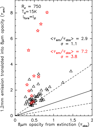
Figure 4: Plot of the 8$\mu$m opacity estimated from the 8$\mu$m Spitzer maps ($\tau_{\rm{abs}}$) and from the 1.2mm dust continuum emission ($\tau_{\rm{em}}$). The starless sources are marked with open triangles while those associated with 24$\mu$m point-like emission are marked with red open star symbols. $\tau_{\rm{abs}}$ has been calculated assuming $I_{\rm{fore}}=I_{\rm{zl}}$. The solid line marks the relationship $\tau_{\rm{abs}}=\tau_{\rm{em}}$, while the two dashed lines indicates $\tau_{\rm{abs}}=0.5\times\tau_{\rm{em}}$ and $\tau_{\rm{abs}}=2\times\tau_{\rm{em}}$

Assuming that for starless cores the true 8$\mu$m opacity is given by $\tau_{\rm{em}}$, we can invert Eq. (2) to estimate the value of I_fore in terms of $I_{\rm{MIR}}$. We did such a calculation for every starless core and plotted the results in Fig. 5, I_MIR being measured at the position of the core on the large scale emission map (Sec. 3.3). A strong correlation is seen between I_fore vs I_MIR. The best linear fit to this correlation is given by

$$I_{\rm{fore}}=0.54\times I_{\rm{MIR}}$$ (5)

with a standard deviation of 0.08, minimum and maximum values of 0.4 and 0.75, respectively. This relationship allows us to compute an average foreground emission just by estimating the mid-infrared radiation for any IRDCs. Figure 6 shows $\tau_{\rm{em}}$ versus $\tau_{\rm{abs}}$ calculated using Eq. (5), but only for the starless cores this time. Here $<\tau_{\rm{em}}/\tau_{\rm{abs}}>=1.1$ with a dispersion of only 0.5.

The relation in Eq. (5) gives us the maximum opacity (and equivalent column density) we can probe before reaching saturation. Indeed, the rms noise level of the 8$\mu$m images ($\sigma_{\rm{noise}}\sim 0.3$ MJy/sr) defines the minimum flux we can detect above the foreground emission. Below this value, the dust in the cloud is basically absorbing all the background emission and we cannot recover the true peak column density. This saturation opacity, $\tau_{\rm{sat}}$, is given by $\tau_{\rm{sat}}=-\ln(\sigma_{\rm{noise}}/I_{\rm{bg}})$, with $I_{\rm{bg}}=0.46\times I_{\rm{MIR}}$. The saturation opacity is calculated for every IRDC and given in Table 1. We also note that we have $I_{\rm{fore}}\simeq I_{\rm{bg}}$ as also observed by Johnstone et al. (2003) and this suggests that most of the foreground emission originates from the same place as the background emission and is local to the IRDC, and therefore the foreground emission is independent of distance to the IRDC.

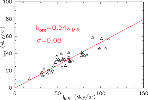
Figure 5: Plot of the 8$\mu$m foreground intensity calculated for 57 positions (see text) of the Rathborne et al. (2006) sample in function of the 8$\mu$m mid-infrared radiation field estimated around them. The best linear fit is shown as a red solid line.

Figure 6: Same as Fig. 4 but only for starless sources and with a 8$\mu$m opacity calculated with $I_{\rm{fore}}=0.54\times I_{\rm{min}}$. The solid line marks the relationship $\tau_{\rm{abs}}=\tau_{\rm{em}}$, while the two dashed lines indicate $\tau_{\rm{abs}}=0.5\times\tau_{\rm{em}}$ and $\tau_{\rm{abs}}=2\times\tau_{\rm{em}}$.

3.3 Construction of the opacity maps

To construct opacity maps of IRDCs all over the Galactic plane we mosaiced the GLIMPSE 8$\mu$m  and MIPSGAL 24$\mu$m images in blocks of $1^{\circ}$ in longitude by $2^{\circ}$ in latitude using the Montage software (http://montage.ipac.caltech.edu/). To allow the identification of IRDCs which cross the edges of these blocks and to allow the extraction of regions large enough for our analysis around clouds near the edges of these blocks, each consecutive block overlaps adjacent blocks by 0.5^∘. In principle this means our extraction could miss IRDCs larger than about $0.5^{\circ}$ in size. However the largest cloud identified by Simon et al. (2006a) is 27^′ long.

The sensitivity of the Spitzer images is such that significant numbers of stars and galaxies appear in them, even at 8$\mu$m. These need to be removed in order to produce clean mid-infrared images and opacity maps of the clouds. This has been done in two steps. First identifying the central position of stars in the field using the IDL FIND task from the Astronomy library. Second, the values in the pixels containing the star were replaced with values calculated from an average gradient plane fit to the values of the pixels surrounding the star we want to remove. While this allowed the recovery of some part of the structure of a cloud, it can also produce artifacts.

Once the 8$\mu$m stars were removed, we calculated the mid-infrared radiation field $I_{\rm{MIR}}$ by smoothing each 8$\mu$m block by a normalised Gaussian of FWHM=308^′′. This size is a compromise between several parameters: the typical size of an IRDC, the typical spatial scale of the 8$\mu$m emission of the Galactic plane and the computation time. Visual inspection of Spitzer images suggests that most of the clouds are filamentary with a minor axis which is not larger than a few arcminutes. The smoothing we have used is well matched to such clouds and our method will recover their exact structure. For clouds which are larger than the smoothing length, but which are centrally condensed, we will detect them but somewhat underestimate their opacity. On the other hand shallow large clouds will be missed (Section 5 and 6). Using a larger smoothing length would allow us to better detect these large clouds, but at the cost of additional processing time and more significantly, the introduction of spurious artificial clouds, especially where the background emission is weak. In any case, distinguishing between a feature due to a smooth lack of background emission or the presence of a large and low column density cloud requires observations of tracers in addition to the inferred mid-infrared extinction. We preferred to convolve the images with a Gaussian rather than using a median filter in order to better recover potential clouds adjacent to strong 8$\mu$m emitting structures.

Having calculated $I_{\rm{MIR}}$ we are able to compute both I_fore and I_bg images (Section 3.2). Then using Eq. (2) we can construct the 8$\mu$m opacity image, but before doing so, we smoothed the 8$\mu$m images with a 4^′′ Gaussian in order to suppress high frequency noise.

A series of artifacts, and spurious clouds may arise from our method. The first one comes from potentially interpreting every decrease in the 8$\mu$m emission on spatial scale smaller than $\sim 5\hbox{${}^{\prime}$}$ as being a potential cloud. This effect is especially important at high latitudes where the mid-infrared radiation field is low. In these regions a small decrease in the intensity will be interpreted as a stronger increase in the opacity than for a similar intensity drop in a high mid-infrared radiation field environment. Identifying such spurious clouds is difficult, and only follow-ups in other tracers in emission will give a definitive answer on the nature of these sources. However, we have attempted to minimise such objects by selecting a relatively high opacity detection threshold.

Another artifact can arise in regions with strong intensity gradients in the initial 8$\mu$m block where the smoothing may artifially produce features identified as clouds, although real clouds also exist in these environments (Deharveng et al., 2009). To help identify possible spurious objects in regions of large 8$\mu$m intensity variations, our catalogue (Table 1) lists $\delta\rm{I_{MIR}}$, the normalised maximum variation of $I_{\rm{MIR}}$ within the IRDC and defined as $\delta I_{\rm{MIR}}=(I_{\rm{MIR}}^{\rm{max}}-I_{\rm{MIR}}^{\rm{min}})/I_{\rm{MIR}}^{\rm{min}}$. Our experience suggests that clouds with $\delta I_{\rm{MIR}}>0.5$ have to be treated with caution. These clouds represent 14% of the total number of IRDCs included in our sample. Overall, after a visual inspection of every IRDC and the removal of obviously spurious IRDCs, we believe that more than 90% of the catalogued objects are true IRDCs.

The tools to automatically construct the maps were mainly constructed using IDL packages.

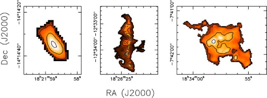
Figure 7: 8$\mu$m opacity maps for the 3 IRDCs showed in Fig. 1. The contours go from 0.4 to 0.8 in steps of 0.2 for the figures on the right and left, while for the middle figure the contours go from 0.4 to to 1.9 in steps of 0.3.

4 From 8$\mu$m opacities to column densities

The images resulting from the analysis described above provide the spatial 8$\mu$m opacity distribution towards IRDCs. However a more useful quantity is the H₂ column density distribution of these clouds. To convert 8$\mu$m opacities to H₂ column densities requires a knowledge of the properties of the absorbing dust. Depending on the line of sight and on the structures observed e.g. diffuse material or dense material, the dust chemical composition and thus, the dust properties, are different. In dense clouds like IRDCs, it is believed that dust grains are larger than in the diffuse interstellar medium due to coagulation and presence of icy mantles on the grains. This is supported by ISO (Lutz et al., 1996), and more recently Spitzer (Indebetouw et al., 2005; Román-Zúñiga et al., 2007), observations which have shown that towards dense clouds, the extinction cannot be fitted by a single power-law from the near-IR up to the mid-IR (Draine & Lee, 1984). The recent work has shown that in dense clouds the extinction decreases from the near infrared to $\sim 5\mu$m and then reaches a plateau up to the silicate absorption band around 9$\mu$m. This behavior can be reproduced with dust models having $R_{v}\simeq 5$ (Weingartner & Draine, 2001), implying larger dust grains (compared to the commonly used value $R_{v}\simeq 3$ for diffuse interstellar medium).

For the IRDCs we therefore adopt a value of $A_{8\mu\rm{m}}/A_{v}=0.045$ (Indebetouw et al., 2005; Román-Zúñiga et al., 2007). To convert to the molecular hydrogen column density, $N_{\rm{H_{2}}}$ we adopt

$$A_{v}=10^{-21}\times N_{\rm{H_{2}}}$$ (6)

from Bohlin et al. (1978), although the more recent work by Draine (2003), based on the observations of Rachford et al. (2002), suggests a 50% larger column density per magnitude of extinction. To account for this, and other uncertainties, the column densities in this (and subsequent papers), have been calculated from the 8$\mu$m optical depth adopting the relation

$$N_{\rm{H_{2}}}=\tau_{8\mu\rm{m}}\times 3[\pm 1]\times 10^{22}\rm{cm}^{-2}$$ (7)

5 Identification of sources

Once the opacity maps have been constructed, we need to extract the information on the structures lying within them. For this purpose, we have developed a new code, largely inspired by the CLUMPFIND source extraction code of Williams et al. (1994). The operation of the code is described in Appendix A. The main differences compared to CLUMPFIND are how a source is defined and its properties determined. This new method does not assume that every pixel belongs to a source, but we define the boundaries of an object by the local minimum between closest neighbours. Then to estimate the size of the source we calculate the first and second order moments of the absorption distribution, and then we diagonalise the second order moment matrix (Appendix A).

5.1 IRDCs

In our maps, the IRDCs have been defined as connected structures lying above an opacity, $\tau_{8\mu\rm{m}}$, of 0.35 with a peak above 0.7 and a diameter greater than 4^′′. Therefore, using Eq. (7), these detection thresholds correspond to $1\times 10^{22}$ cm^-2 and $2\times 10^{22}$ cm^-2, respectively. With these parameters, we have identified 11303 IRDCs (see Fig. 7). Table 1 lists the first 30 IRDCs, giving their name, coordinates, I_min in MJy/sr, I_MIR in MJy/sr, $\delta{\rm I_{MIR}}$ (see Sec. 3.3), $\Delta X$ the major axis size in arcseconds, $\Delta Y$ the minor axis size in arcseconds, $\alpha$ the position angle in degrees ( see Appendix A for an exact definition of these parameters), R_eq the equivalent radius which corresponds to the radius of a disc having the same area as the IRDC in arcseconds, $\tau_{\rm{peak}}$ the 8$\mu$m peak opacity, $\tau_{\rm{av}}$ the $8\mu$m opacity averaged over the cloud, $\tau_{\rm{sat}}$ the saturation opacity as described in Section 3.2, the number of fragments within the IRDC (Sec. 5.2), whether there is a 24$\mu$m star in the field/IRDC or not (Sec. 5.3), and $\sigma_{\rm{star}}$ the 24$\mu$m stellar density around the IRDC in number of stars per arcminute squared.

5.2 IRDC fragments

Substructures are seen in almost every IRDC map (Fig. 7). Since column density peaks likely pinpoint the sites of the formation of the next generation of stars, identifying these peaks is crucial in identifying the initial conditions of star formation in IRDCs. We call these substructures identified within the IRDCs fragments. We prefer this name, rather than for example, cores, as they have been called in other papers (e.g. Rathborne et al., 2006). The term core has often been used to identify a substructure which forms one star or a small group of stars and we do not at this stage wish to imply any physical interpretation of these structures in IRDCs. Especially since we do not know the distance of the bulk of the IRDCs, we cannot infer any physical parameters such as the sizes and masses of the fragments/IRDCs.

To extract the IRDC fragments, we apply the same extraction code used to identify the IRDCs (Appendix A). We applied different values of $\tau_{\rm{step}}$ in order to get a comprehensive picture of the fragmentation in these IRDCs. In total we identified 20000 to 50000 fragments depending on $\tau_{\rm{step}}$ (from 0.1 to 0.35). For each of these fragments we have measured their positions, sizes, peak and average opacity, and their 24$\mu$m star association. As an indication of the degree of fragmentation Table 1 includes the number of fragments extracted in each IRDC with $\tau_{\rm{step}}=0.35$. The nature of these fragments is discussed in detail in Peretto & Fuller (2009, in preparation).

Table 2: Average properties of IRDCs and fragments (extracted with $\tau_{\rm{step}}=0.35$).

Structures	Number of	Req		Aspect ratio		$\tau_{\rm{av}}$		$\tau_{\rm{peak}}$		Star association
	Objects	Average	Range	Average	Range	Average	Range	Average	Range
		(arcsec)	(arcsec)							$\%$
IRDCs	11303	31	4–374	2.2	1.0–11.6	0.15	0.01–2.35	1.15	0.70 – 8.36	20-68
Fragments	19838	19	1–205	2.0	1.0–11.6	0.75	0.01–7.88	1.63	0.70 – 8.36	6

5.3 24$\mu$m point-like sources association

In order to check for star formation activity associated with the IRDCs and fragments, we analysed the 24$\mu$m MIPSGAL data, looking for point-like sources. For this purpose we used the IDL FIND task of the IDL Astronomy Library. As an initial indication of the the star formation activity of these IRDCs, we have identified all the 24$\mu$m stars lying within a box (described as Field in Table 1 col. 16) of twice the calculated extent along the coordinate axes of each IRDC. Doing so, we find that 32$\%$ of the IRDCs do not have any 24$\mu$m point-like sources in such a box. On the other hand, 20$\%$ of the IRDCs have a 24$\mu$m source lying within their boundaries (Table 1 col. 17). Therefore, the percentage of active star forming IRDCs is likely to be between 20 and 68$\%$. A more detailed analysis of the stellar content of IRDCs will be presented in a following paper.

Concerning the fragments, between 1% and 6% have stars lying within their boundaries, depending on the parameters used to extract the fragments (Peretto & Fuller 2009, in preparation).

We have also calculated the 24$\mu$m stellar surface density around each IRDC extracted (Table 2 col. 18). This number provides an idea of the crowding in the area around the IRDC.

5.4 Uncertainties on the opacity estimates

The main source of uncertainty in the opacity maps arises from the estimate of the foreground intensity $I_{\rm{fore}}$. As explained in Section 3, we used the relation $I_{\rm{fore}}=0.54\times I_{\rm{MIR}}$ to calculate this quantity for every cloud. However, as can be seen in Fig. 5 a dispersion of $\sim 0.1$ exists on this relation with a maximum variation of $\pm 0.25$. To assess the impact of such variations on the calculated peak opacities of the clouds we have computed for every cloud the ratio, $K$, of the peak opacity inferred assuming $I_{\rm{fore}}=C_{f}\times I_{\rm{MIR}}$ where $0.25<C_{f}<0.75$ to the peak opacity calculated with the fiducial $I_{\rm{fore}}$ (Eq. 5; $C_{f}=0.54$). Figure 8 shows the median value of this ratio as a function of $C_{f}$. For each value of $C_{f}$ we also calculated the dispersion in $K$ across the entire sample of clouds. These dispersions were all $<0.1$, except for the case $C_{f}=0.75$ where the dispersion in $K$ reached 0.3. The range in $K$ shown on Fig. 8 provides an estimate of the peak opacity uncertainty related to the choice/variation of $I_{\rm{fore}}$. In most cases this uncertainty is less than a factor of 2, but can be as large as 10 for extreme cases. On the same figure we also plot the fraction of saturated clouds in function of the adopted $I_{\rm{fore}}$. Naturally, the higher $I_{\rm{fore}}$, the higher the number of saturated clouds, reaching 80$\%$ in the most extreme case, but being less than 10$\%$ for $I_{\rm{fore}}<0.6\rm{I}_{\rm{MIR}}$. In the case of $C_{f}=0.54$, the percentage of saturated cloud is $3\%$. This is consistent with a visual inspection of the 8$\mu$m intensity profiles of a sample of clouds which indicates that less than 10% of the objects show a flattening in their inner regions, a signature of possible saturation.

Another source of uncertainty is the variation of the foreground intensity relative to the background emission. Since we have shown that on average the background emission is equal to the foreground emission (Sec. 3.2), we assumed that the variations of both quantities in front and behind a cloud have the same origin, and so, the same variations. However, this assumption could be wrong. For instance one could be constant over the extent of the cloud, more likely the foreground, with the other one containing all the variations observed in the mid-infrared radiation field. The impact of such effects on the opacity estimate is similar to the one described above. Clouds with small variations in their mid-infrared radiation fields are thus better constrained than the ones with high $\delta I_{\rm{MIR}}$.

As mentioned in the previous section large clouds ($>5\hbox{${}^{\prime}$}$) have opacities which are likely to be underestimated, however this effect is minor compared with those mentioned above. Overall, considering all the factors which contribute to the uncertainty in opacity, we estimate the values derived from the Spitzer data are uncertain by a factor of no more than two. This result is consistent with the observations of a subset of clouds in the 1.2mm continuum emission from the dust (Fig. 6).

Figure 8: (top): Correction factor to apply to peak opacities in order to correct for different foreground intensities than the one we used in this study. (bottom): Fraction of saturated clouds as a function of the assumption made on the foreground intensity.

6 Comparison with the MSX IRDC catalogue

Simon et al. (2006a) undertook a systematic survey of IRDCs using MSX data. Their survey covers a larger area of the Galactic plane than ours due to the smaller coverage of GLIMPSE survey. In total, Simon et al. (2006a) have extracted 6721 clouds between $10\hbox{${}^{\circ}$}<|l|<65\hbox{${}^{\circ}$}$ and $-1\hbox{${}^{\circ}$}<b<1\hbox{${}^{\circ}$}$. For the same coverage we extracted 11303 Spitzer dark clouds, which is roughly twice as many. However, the detection limits, peak and boundary, in the two surveys are different, the simple comparison of the numbers of clouds provides only an incomplete comparison and so a more complete comparison has been performed.

As illustrated by Fig. 9, it appears that a minority of IRDCs are common to both MSX and Spitzer catalogues. Actually, only 20$\%$ of the Spitzer dark clouds appear in the MSX catalogue (corresponding to 25$\%$ of MSX clouds being associated with a Spitzer dark cloud). Based on this comparison we define 3 categories of clouds: Spitzer only, which are clouds appearing only in our catalogue; MSX only, which are clouds appearing only in Simon et al. catalogue; and both, which are clouds appearing in both catalogues. Figure 10 shows an example of an IRDC in each of these categories.

Of the Spitzer only clouds, 51% do not meet the size criteria, R${}_{eq}>20\hbox{${}^{\prime\prime}$}$, imposed by Simon et al. (2006a) to identify the MSX IRDCs, explaining why they are not in the MSX catalogue. The remaining $\sim 30\%$ of Spitzer only IRDCs are the result from the difference in the method used to estimate the background. Using a median filter of 30^′ diameter, Simon et al. (2006a) underestimated the background almost everywhere in the inner $0<|b|<0.25\hbox{${}^{\circ}$}$ of the Galactic plane. As a consequence, the inferred background reaches a similar value as the IRDC itself, and therefore, an IRDC is not detected. This artifact can be seen when ploting the source fraction as a function of the Galactic latitude (Fig. 11). We see a significant difference between the distributions of MSX and Spitzer IRDCs. The MSX IRDCs have a rather flat distribution in a central 1^∘ region whereas the Spitzer IRDC distribution has a clear central peak decreasing sharply on both sides of it. We believe than this difference arises from the difference in the background construction.

On the other hand the MSX only clouds have very low contrast (opacity peaks) and are particularly large. The detection of such clouds in the MSX data has been possible due to the large background smoothing length, and the low contrast threshold used by Simon et al. (2006a). In order to investigate this effect and see whether our method could recover these clouds when using a larger Gaussian, we smoothed the block shown in Fig 9 to 20^′, and performed the extraction of IRDCs on the resulting opacity map. Doing so, we find twice as many clouds (40%) which are in both catalogues, but in parallel 35% of Spitzer clouds which were initially detected using a smaller Gaussian are lost. The remaining MSX only clouds are just too shallow to be identified given the opacity threshold we used, 0.7. In addition, looking at their 8$\mu$m emission it is not clear whether many of these clouds are real, or just a decrease in the background of the Galactic plane.

Overall, we can say that 80% of our catalogue comprises IRDCs which were previously unknown and constitutes the most complete catalogue available of such objects with column density peaks above $1\times 10^{22}$ cm^-2.

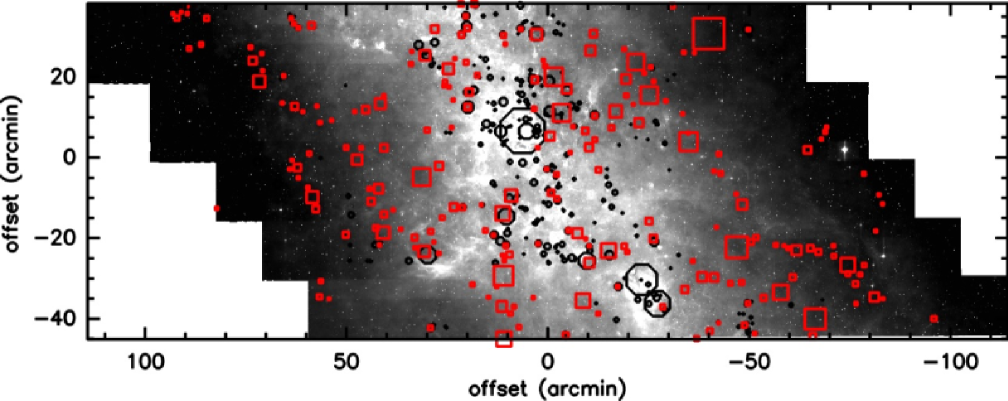
Figure 9: In grey scale is the Spitzer 8$\mu$m emission of one of the blocks we constructed around $l\simeq 30\hbox{${}^{\circ}$}$. The black circles indicate the position and size of the Spitzer IRDCs identified in this study, while the red square symbols code the position and size of the MSX IRDCs. We see on this image that the Spitzer IRDCs are more numerous where the background is stronger, while, quite surprisingly, this is not the case for the MSX IRDCs. The MSX clouds detected at $|b|>0.5\hbox{${}^{\circ}$}$, are on average the larger clouds in the Simon et al. (2006a) sample. For most of them, we do not detect any Spitzer IRDCs at these positions in our standard processing (using a 5^′ Gaussian) but some are detected when using a larger smoothing function (see text).

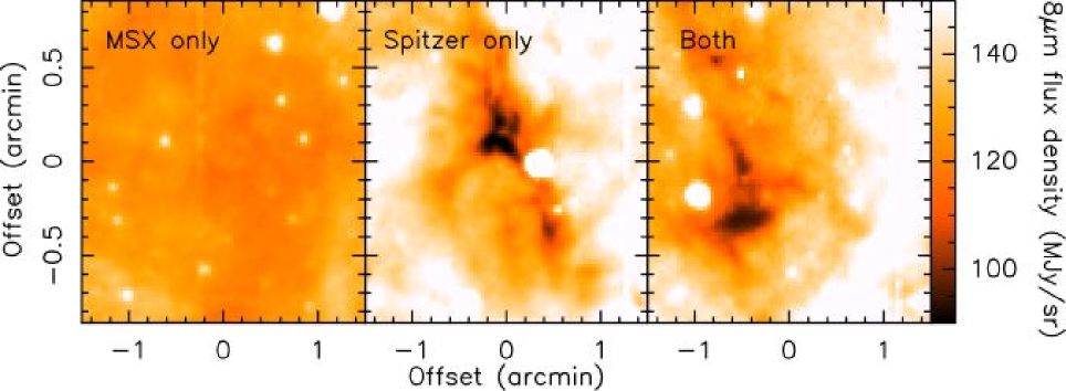
Figure 10: Comparison of three IRDCs seen with Spitzer at 8$\mu$m illustrating the 3 categories of IRDC based on their MSX and Spitzer detection. Note that the cloud detected only in the MSX catalogue (left panel) exhibits much lower extinction than the other two objects.

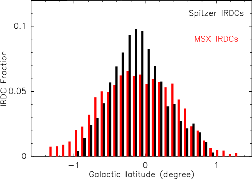
Figure 11: Comparison of the latitude distribution of Spitzer and MSX dark clouds

7 Summary

This paper, the first of a series dedicated to the study of infrared dark clouds, describes the techniques developed to establish a complete catalogue of Spitzer dark clouds. We analysed the full data set of the 8$\mu$m GLIMPSE Galactic plane to look for IRDCs. We extracted 11303 of these clouds, obtaining column density maps for each of them, and characterizing their physical properties. We also identify the substructures lying within these clouds, extracting up to $\sim 50000$ of these. Table 2 presents a summary of the average and range of properties of both the clouds and these substructures (fragments). The full table of the properties of the clouds and fragments plus images and opacity maps are available from an online database. In subsequent papers we will exploit the tremendous quantity of information concerning the initial conditions for the formation of stars in the Galaxy contained within this set of IRDC column density maps.

Appendix A Method for extracting sources

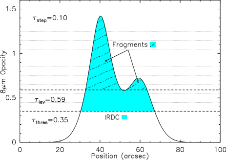
Figure 12: Illustration of our extraction method. This figure shows the opacity profile of a typical IRDC. The bottom dashed line shows the opacity threshold beneath which structures are ignored. The dotted lines show the different slices through the cloud, every slice being separated by $\tau_{\rm{step}}$. The upper dashed line shows the opacity corresponding to the local minimum , $\tau_{\rm{lev}}$, between the two local peaks shown on that plot. In such a cloud, our method would extract one IRDC (colored area) and two fragments (colored area + dashed-dotted lines) within it.

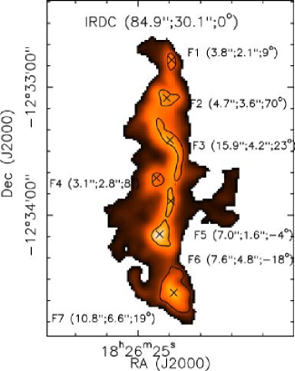
Figure 13: 8$\mu$m opacity map of the middle IRDC shown in Fig. 1. Our extraction method detected 7 fragments within this IRDCs when $\tau_{\rm{step}}=0.1$. The black contours mark the $\tau_{\rm{lev}}$ value (boundary contour) for each fragment. The sizes and position angle are also given in between brackets. We can see that these values give a reasonable description of the shape of the fragments (and IRDC)

We developed a new code to extract sources from our opacity maps. The first part of our algorithm is mainly based on the same principle as the one developed by Williams et al. (1994) for CLUMPFIND. We set two main parameters which are the lowest contour level under which we do not consider any structure, $\tau_{\rm{thres}}$, and a step in unit of the map, $\tau_{\rm{step}}$. Then we look at every local peak between two consecutive levels, up to the maximum of our image. The number of local peaks gives us the number of fragments we will extract from the image, unless the final estimated size is lower than the final angular resolution or that the amplitude between the peak of the fragment and its external boundary is less than $\tau_{\rm{step}}$. Then we have to determine the pixels we associate to each local peak. For this, for every peak, we go down, level by level, and check if the local peak we are looking at is the only one in this contour. If yes, we look at the following contour and do the same job. If there is more than one local peak within the contour we look for the local minimum between these two peaks, $\tau_{\rm{lev}}$, and the pixels lying above $\tau_{\rm{lev}}$ and associated with the considered peak define the extent of the fragment.

In order to measure the size of the clouds and fragments, we did not want to assume any particular shape for the source. So, once we have identify all the pixels associated with a given peak, we estimate first the center of gravity of the cores, $(X_{CG},Y_{CG})$, using

$$X_{CG}=\frac{\displaystyle\sum_{i=1}^{N}V_{i}\times x_{i}}{\displaystyle\sum_{i=1}^{N}V_{i}}\\ Y_{CG}=\frac{\displaystyle\sum_{i=1}^{N}V_{i}\times y_{i}}{\displaystyle\sum_{i=1}^{N}V_{i}}$$ (8)

where $V_{i}$ is the value of the $i$th pixel, $x_{i}$ and $y_{i}$ its coordinates, and N is the number of pixels. Then, we calculate the matrix of moment of inertia, I:

$$I=\left[\begin{array}[]{cc}I_{xx}&I_{xy}\\ I_{yx}&I_{yy}\\ \end{array}\right]$$ (9)

with

$$I_{xx}=\displaystyle\sum_{i=1}^{N}V_{i}(y_{i}-Y_{CG})^{2}\\$$ (10)

$$I_{yy}=-\displaystyle\sum_{i=1}^{N}V_{i}(x_{i}-X_{CG})^{2}\\$$ (11)

$$I_{xy}=I_{yx}=\displaystyle\sum_{i=1}^{N}V_{i}(x_{i}-X_{CG})(y_{i}-Y_{CG})$$ (12)

Finally, we diagonalize I in order to obtain its two eigenvalues and eigenvectors. From this we can easily calculate the position angle $\alpha$ of the major axis (given by the vector associated by the smallest eigenvalue). To estimate the sizes of the cores we calculate the following values:

$$\sigma_{X}^{2}=\displaystyle\sum_{i=1}^{N}\left(\left[x_{i}\cos(\alpha)-y_{i}\sin(\alpha)\right]-\left[X_{CG}\cos(\alpha)-Y_{CG}\sin(\alpha)\right]\right)^{2}$$ (13)

$$\sigma_{Y}^{2}=\displaystyle\sum_{i=1}^{N}\left(\left[x_{i}\sin(\alpha)+y_{i}\cos(\alpha)\right]-\left[X_{CG}\sin(\alpha)+Y_{CG}\cos(\alpha)\right]\right)^{2}$$ (14)

The sizes are then estimated by $\Delta X=2\times\sqrt{\sigma_{X}^{2}/N}$ and $\Delta Y=2\times\sqrt{\sigma_{Y}^{2}/N}$

The three values, $\Delta X$, $\Delta Y$ and $\alpha$, are given for every IRDC in Table 1.

References

- André et al. (2007) André, P., Belloche, A., Motte, F., & Peretto, N. 2007, A&A, 472, 519
- Bacmann et al. (2000) Bacmann, A., André, P., Puget, J.-L., et al. 2000, A&A, 361, 555
- Bally et al. (2006) Bally, J., Walawender, J., Luhman, K. L., & Fazio, G. 2006, AJ, 132, 1923
- Blitz (1993) Blitz, L. 1993, in Protostars and Planets III, ed. E. H. Levy & J. I. Lunine, 125–161
- Bohlin et al. (1978) Bohlin, R. C., Savage, B. D., & Drake, J. F. 1978, ApJ, 224, 132
- Carey et al. (1998) Carey, S. J., Clark, F. O., Egan, M. P., et al. 1998, ApJ, 508, 721
- Deharveng et al. (2009) Deharveng, L., Zavagno, A., Schuller, F., et al. 2009, A&A, 496, 177
- Draine (2003) Draine, B. T. 2003, ARA&A, 41, 241
- Draine & Lee (1984) Draine, B. T. & Lee, H. M. 1984, ApJ, 285, 89
- Egan et al. (1998) Egan, M. P., Shipman, R. F., Price, S. D., et al. 1998, ApJ, 494, L199+
- Enoch et al. (2006) Enoch, M. L., Young, K. E., Glenn, J., et al. 2006, ApJ, 638, 293
- Hatchell et al. (2005) Hatchell, J., Richer, J. S., Fuller, G. A., et al. 2005, A&A, 440, 151
- Hennebelle et al. (2001) Hennebelle, P., Pérault, M., Teyssier, D., & Ganesh, S. 2001, A&A, 365, 598
- Indebetouw et al. (2005) Indebetouw, R., Mathis, J. S., Babler, B. L., et al. 2005, ApJ, 619, 931
- Johnstone et al. (2003) Johnstone, D., Fiege, J. D., Redman, R. O., Feldman, P. A., & Carey, S. J. 2003, ApJ, 588, L37
- Lada & Lada (2003) Lada, C. J. & Lada, E. A. 2003, ARA&A, 41, 57
- Lutz et al. (1996) Lutz, D., Feuchtgruber, H., Genzel, R., et al. 1996, A&A, 315, L269
- Motte et al. (1998) Motte, F., Andre, P., & Neri, R. 1998, A&A, 336, 150
- Ossenkopf & Henning (1994) Ossenkopf, V. & Henning, T. 1994, A&A, 291, 943
- Perault et al. (1996) Perault, M., Omont, A., Simon, G., et al. 1996, A&A, 315, L165
- Peretto et al. (2006) Peretto, N., André, P., & Belloche, A. 2006, A&A, 445, 979
- Pillai et al. (2006) Pillai, T., Wyrowski, F., Carey, S. J., & Menten, K. M. 2006, A&A, 450, 569
- Rachford et al. (2002) Rachford, B. L., Snow, T. P., Tumlinson, J., et al. 2002, ApJ, 577, 221
- Rathborne et al. (2006) Rathborne, J. M., Jackson, J. M., & Simon, R. 2006, ApJ, 641, 389
- Reach et al. (2005) Reach, W. T., Megeath, S. T., Cohen, M., et al. 2005, PASP, 117, 978
- Román-Zúñiga et al. (2007) Román-Zúñiga, C. G., Lada, C. J., Muench, A., & Alves, J. F. 2007, ApJ, 664, 357
- Simon et al. (2006a) Simon, R., Jackson, J. M., Rathborne, J. M., & Chambers, E. T. 2006a, ApJ, 639, 227
- Simon et al. (2006b) Simon, R., Rathborne, J. M., Shah, R. Y., Jackson, J. M., & Chambers, E. T. 2006b, ApJ, 653, 1325
- Teixeira et al. (2006) Teixeira, P. S., Lada, C. J., Young, E. T., et al. 2006, ApJ, 636, L45
- Teyssier et al. (2002) Teyssier, D., Hennebelle, P., & Pérault, M. 2002, A&A, 382, 624
- Weingartner & Draine (2001) Weingartner, J. C. & Draine, B. T. 2001, ApJ, 548, 296
- Williams et al. (1994) Williams, J. P., de Geus, E. J., & Blitz, L. 1994, ApJ, 428, 693