Accuracy of direct gradient sensing by cell-surface receptors

Abstract

Chemotactic cells of eukaryotic organisms are able to accurately sense shallow chemical concentration gradients using cell-surface receptors. This sensing ability is remarkable as cells must be able to spatially resolve small fractional differences in the numbers of particles randomly arriving at cell-surface receptors by diffusion. An additional challenge and source of uncertainty is that particles, once bound and released, may rebind the same or a different receptor, which adds to noise without providing any new information about the environment. We recently derived the fundamental physical limits of gradient sensing using a simple spherical-cell model, but not including explicit particle-receptor kinetics. Here, we use a method based on the fluctuation-dissipation theorem (FDT) to calculate the accuracy of gradient sensing by realistic receptors. We derive analytical results for two receptors, as well as two coaxial rings of receptors, e.g. one at each cell pole. For realistic receptors, we find that particle rebinding lowers the accuracy of gradient sensing, in line with our previous results.

I Introduction

Cells are able to sense gradients of chemical concentration with extremely high sensitivity and accuracy. This is done either directly, by measuring spatial gradients across the cell diameter, or indirectly, by temporally sensing gradients while moving dusenbery98 . In temporal sensing, a cell modifies its swimming behavior according to whether a chemical concentration is rising or falling in time berg99 . This mode of sensing is typical of small, fast moving bacteria such as Escherichia coli, which can respond to changes in concentration as low as 3.2 nM of the attractant aspartate manson03 . In contrast, direct spatial sensing is prevalent among larger, single-celled eukaryotic organisms such as the slime mold Dictyostelium discoideum (Dicty) and the budding yeast Saccharomyces cerevisiae arkowitz99 ; manahan04 . Dicty cells are able to sense a concentration difference of only 1-5% across the cell mato75 , corresponding to a difference in receptor occupancy between front and back of only 5 receptors haastert07 . Spatial sensing is also performed by cells of the immune system including neutrophils and lymphocytes zigmond77 , as well as by growing synaptic cells and tumor cells. Interestingly, a direct spatial mode of sensing has also been demonstrated for the large oxygen-sensing bacterium Thiovulum majus thar03 , indicating that direct gradient sensing is widespread among the different kingdoms of life.

There has been great progress in understanding the limits of concentration sensing in bacteria such as E. coli, pioneered by Berg berg77 ; berg99 ; sourjik2002 , and in understanding the origins of sensitivity in the underlying signaling network, pioneered by Bray bray98 ; duke99 ; bray02 ; bray07 , and followed by others SB2004 ; mello05 ; keymer06 ; endres06 ; bialek08 ; hansen08 ; endres_MSB08 . By contrast, very little is known about what determines the accuracy of direct gradient sensing by eukaryotic cells. Recently, we derived the fundamental physical limits of direct gradient sensing, where the accuracy is limited by the random arrival of particles at the cell surface due to diffusion endres_PNAS08 . We used as models a perfectly absorbing sphere and a perfectly monitoring sphere (à la Berg and Purcell berg77 ). In these two models, gradients are inferred from the positions of particles absorbed on the surface of a sphere or the positions of freely diffusing particles inside a spherical volume, respectively. The latter case simulates rebinding of particles, as particles can enter and exit the spherical volume freely. In comparison, for the perfectly absorbing sphere, previously observed particles are never remeasured. As a result, we found that the perfectly absorbing sphere is superior to the perfectly monitoring sphere, both for concentration and gradient sensing (Table I).

The superiority of the absorbing sphere may help explain the presence at the surfaces of cells of signal degrading enzymes, such as PDE for cAMP in Dicty and BAR1 for mating factor $\alpha$ in S. cerevisiae. Those surface enzymes could reduce or eliminate rebinding (and therefore remeasurement) of the same signal molecule. Quantitatively, our theory compares favorably to recent measurements of Dicty moving up shallow cAMP gradients haastert07 , suggesting that these cells operate near the physical limits of gradient detection.

While our recent models of the absorbing and monitoring spheres allowed us to derive the fundamental limit of gradient sensing, the models neglect the details of biochemical reactions, such as particle-receptor binding and downstream signaling events, which might further increase measurement uncertainty. To study the effects of particle-receptor binding, we here extend a formalism for the uncertainty of concentration sensing recently developed by Bialek and Setayeshgar bialek05 ; bialek08 , to the case of gradient sensing. This formalism uses the fluctuation-dissipation theorem to infer the fluctuations of the receptor occupancy (and hence the accuracy of concentration sensing) from the linear response of the average receptor occupancy to changes in receptor binding free energies. The effect of particle rebinding is included by coupling particle-receptor binding to the diffusion equation bialek05 , leading to correlations in time among the receptors. We report analytical results for two receptors (Fig. 1), as well as two coaxial rings of receptors, e.g. one at each cell pole (Fig. 2). By assuming diffusion-limited particle binding to the receptors, we are able to directly compare to our previous model for the fundamental limits of gradient sensing. For realistic receptors, we find that particle rebinding lowers the accuracy of gradient sensing in line with our previous results for the absorbing and monitoring spheres (Table I).

Measurement uncertainty	Perfect absorber	Perfect monitor	Ratio absorber/monitor
Concentration: $\frac{\langle(\delta c)^{2}\rangle}{c_{0}^{2}}$	$\frac{1}{4\pi Dac_{0}T}$	$\frac{3}{5\pi Dac_{0}T}$ berg77	$\frac{12}{5}$$=2.4$
Gradient: $\frac{\langle(\delta c_{\vec{r}})^{2}\rangle}{(c_{0}/a)^{2}}$	$\frac{1}{4\pi Dac_{0}T}$	$\frac{15}{7\pi Dac_{0}T}$	$\frac{60}{7}$$\approx 8.6$

Table 1: Uncertainties in measured concentration and concentration gradient for two idealized cell models: a perfectly absorbing sphere (second column) and a perfectly monitoring sphere (third column). Also provided is the ratio of the uncertainties of the absorber and monitor. Parameters: diffusion constant $D$, radius of sphere $a$, averaging time $T$, and average chemical concentration $c_{0}$. Table reproduced from Ref. endres_PNAS08 .

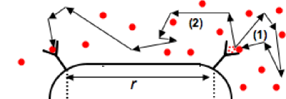
Figure 1: Model for gradient sensing by two individual cell-surface receptors. Particles diffuse through the medium and randomly bind to and unbind from receptors, e.g. see the two sample paths indicated by black arrows. Particles may rebind the same (1) or a different (2) receptor. The receptor separation is given by $r$.

II Methods

Bialek and Setayeshgar bialek05 previously presented a method based on the fluctuation-dissipation theorem (FDT) kubo66 to calculate the accuracy of measurement of chemical concentration by receptors. We extend their method to calculate the accuracy of measurement of concentration gradients, and derive analytical results for (1) two receptors and (2) two coaxial rings of receptors, e.g. one at each cell pole. We start our derivation by considering an arbitrary number $m$ of receptors.

The kinetics of the ensemble-average occupancy $n_{j}(t)$ of receptor $j$ due to binding and unbinding of chemical ligands at the local concentration $c(\vec{x}_{j},t)$ is given by

$$\frac{dn_{j}(t)}{dt}=k_{+}c(\vec{x}_{j},t)[1-n_{j}(t)]-k_{-}n_{j}(t).$$ (1)

Linearization about the mean steady-state occupancy $\bar{n}_{j}=k_{+}\bar{c}_{j}/(k_{+}\bar{c}_{j}+k_{-})$ at concentration $\bar{c}_{j}=\bar{c}(\vec{x}_{j},t)$ gives

$$\frac{d(\delta n_{j}(t))}{dt}=-(k_{+}\bar{c}_{j}+k_{-})\delta n_{j}+\bar{c}_{j}(1-\bar{n}_{j})\delta k_{+}-\bar{n}_{j}\delta k_{-}+k_{+}(1-\bar{n}_{j})\delta c_{j}.$$ (2)

By thermodynamics, the ratio of binding and unbinding rates is related to the free-energy difference $F_{j}$ between the unbound and bound states of the receptor according to

$$\frac{k_{+}\bar{c}_{j}}{k_{-}}=\exp\left(\frac{F_{j}}{k_{B}T}\right).$$ (3)

Variations of the rate constants in Eq. 2 are equivalent to a variation or external perturbation of this receptor free-energy difference

$$\frac{\delta F_{j}}{k_{B}T}=\frac{\delta k_{+}}{k_{+}}-\frac{\delta k_{-}}{k_{-}}.$$ (4)

Combining Eqs. 2 and 4, one obtains after Fourier transforming in time to obtain a frequency representation

$$-i\omega\delta\hat{n}_{j}(\omega)=-(k_{+}\bar{c}_{j}+k_{-})\delta\hat{n}_{j}(\omega)+\frac{k_{+}(1-\bar{n}_{j})\bar{c}_{j}}{k_{B}T}\delta\hat{F}_{j}(\omega)+k_{+}(1-\bar{n}_{j})\delta\hat{c}_{j}(\omega),$$ (5)

where, e.g., $\delta\hat{n}_{j}(\omega)$ describes the variations in the receptor occupancy as a function of frequency $\omega$. The dependence on $\delta\hat{c}_{j}(\omega)$ can be eliminated by using the (linearized) diffusion equation bialek05 in Eq. 5

$$\frac{\partial(\delta c(\vec{x},t))}{\partial t}=D\nabla^{2}\delta c(\vec{x},t)-\sum_{l=1}^{m}\delta(\vec{x}-\vec{x_{l}})\frac{d(\delta n_{l}(t))}{dt}.$$ (6)

Using the Fourier transforms

$$\delta c(\vec{x},t) = \int\frac{d\omega}{2\pi}\int\frac{d^{3}k}{(2\pi)^{3}}e^{i(\vec{k}\vec{x}-\omega t)}\delta\hat{c}(\omega,\vec{k})$$ (7)

$$\delta(\vec{x}-\vec{x}_{l}) = \int\frac{d^{3}k}{(2\pi)^{3}}e^{i\vec{k}(\vec{x}-\vec{x}_{l})-k/\Lambda}$$ (8)

$$\delta n_{l}(t) = \int\frac{d\omega}{2\pi}e^{-i\omega t}\delta\hat{n}_{l}(\omega),$$ (9)

where $k=|\vec{k}|$ and where we have introduced a convergence factor $\Lambda\gtrsim 0$ in Eq. 8 to regulate the $\delta$ function (effectively assigning a size scale $\sim 1/\Lambda$ to the receptor), Eq. 6 yields

$$\delta\hat{c}(\omega,\vec{k})=\frac{i\omega}{Dk^{2}-i\omega}\sum_{l=1}^{m}e^{-i\vec{k}\vec{x}_{l}-k/\Lambda}\delta\hat{n}_{l}(\omega).$$ (10)

Inverting the spatial Fourier transform back into real space, one obtains the concentration fluctuations at the locations of the receptors in terms of the occupancy fluctuations

$$\delta\hat{c}(\vec{x}_{j},\omega) = i\omega\sum_{l=1}^{m}\delta\hat{n}_{l}(\omega)\int\frac{d^{3}k}{(2\pi)^{3}}\frac{e^{i\vec{k}(\vec{x}_{j}-\vec{x}_{l})-k/\Lambda}}{Dk^{2}-i\omega}$$ (11)

$$= i\omega\left[\delta\hat{n}_{j}(\omega)\int\frac{d^{3}k}{(2\pi)^{3}}\frac{e^{-k/\Lambda}}{Dk^{2}-i\omega}+\sum_{l\neq j}^{m}\delta\hat{n}_{l}(\omega)\int\frac{d^{3}k}{(2\pi)^{3}}\frac{e^{i\vec{k}(\vec{x}_{j}-\vec{x}_{l})}}{Dk^{2}-i\omega}\right]$$ (12)

$$= \frac{i\omega}{2\pi^{2}}\left[\delta\hat{n}_{j}(\omega)\int_{0}^{\Lambda}\frac{k^{2}\,dk}{Dk^{2}-i\omega}+\sum_{l\neq j}^{m}\frac{\delta\hat{n}_{l}(\omega)}{|\vec{x}_{j}-\vec{x}_{l}|}\int_{0}^{\infty}\frac{k\sin(k|\vec{x}_{j}-\vec{x}_{l}|)}{Dk^{2}-i\omega}dk\right].$$ (13)

The cut-off $\Lambda=\pi/s$, which accounts for the physical dimensions of the receptor, is used in Eq. 13 to set an upper limit of integration bialek05 .

Following Bialek and Setayeshgar bialek05 , we imagine that the mechanism that reads out the receptor occupancy averages over a time $\tau$ long compared to the correlation time between binding and unbinding events of a receptor (see below). In this case, we can apply the low-frequency limit ($\omega<\!\!<D\Lambda^{2}$). Using the expression

$$\lim_{\omega\rightarrow 0}\frac{1}{v\mp i\omega}=\frac{P}{v}\pm i\pi\delta(0),$$ (14)

where $v$ is real and $P$ is the principal value of the associated integral, Eq. 13 becomes

$$\delta\hat{c}(\vec{x_{j}},\omega)=\frac{i\omega\Lambda}{2\pi^{2}D}\delta\hat{n}_{j}(\omega)+\frac{i\omega}{4\pi D}\sum_{l\neq j}^{m}\frac{\delta\hat{n}_{l}(\omega)}{|\vec{x}_{j}-\vec{x}_{l}|}.$$ (15)

Inserting Eq. 15 for $\delta\hat{c}_{j}(\vec{x},\omega)$ in Eq. 5 yields

$$-i\omega\delta\hat{n}_{j} = \left[k_{+}(1-\bar{n}_{j})\frac{i\omega\Lambda}{2\pi^{2}D}-(k_{+}\bar{c}_{j}+k_{-})\right]\delta\hat{n}_{j}$$ (16)

$$+k_{+}(1-\bar{n}_{j})\frac{i\omega}{4\pi D}\sum_{l\neq j}^{m}\frac{\delta\hat{n}_{l}}{|\vec{x}_{j}-\vec{x}_{l}|}+\frac{k_{+}(1-\bar{n}_{j})\bar{c}_{j}}{k_{B}T}\delta\hat{F}_{j},$$

which depends only on the $\delta\hat{n}_{j}(\omega)$ and their conjugate variables $\delta\hat{F}_{j}(\omega)$. These $m$ equations describe how deterministic frequency-dependent changes in the free-energy differences $\delta\hat{F}_{j}(\omega)$ affect the frequency-dependent occupancies $\delta\hat{n}_{j}(\omega)$ of all the receptors.

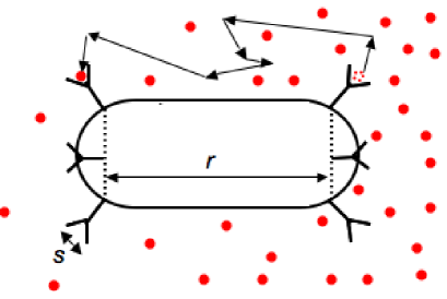
Figure 2: Model for gradient sensing by two polar rings of surface receptors. Particles diffuse through the medium and randomly bind to and unbind from receptors. Particles may rebind the same or different receptors (e.g., path of black arrows). Rings of receptors are separated by distance $r$. Also shown is receptor dimension $s$.

Two receptors
We first consider two identical receptors (Fig. 1) for which Eq. 16 simplifies to two coupled linear equations

$$-i\omega\delta\hat{n}_{1} = \left[k_{+}(1-\bar{n}_{1})\frac{i\omega\Lambda}{2\pi^{2}D}-(k_{+}\bar{c}_{1}+k_{-})\right]\delta\hat{n}_{1}$$ (17)

$$+k_{+}(1-\bar{n}_{1})\frac{i\omega}{4\pi D}\frac{\delta\hat{n}_{2}}{|\vec{x}_{1}-\vec{x}_{2}|}+\frac{k_{+}(1-\bar{n}_{1})\bar{c}_{1}}{k_{B}T}\delta\hat{F}_{1}$$

$$-i\omega\delta\hat{n}_{2} = \left[k_{+}(1-\bar{n}_{2})\frac{i\omega\Lambda}{2\pi^{2}D}-(k_{+}\bar{c}_{2}+k_{-})\right]\delta\hat{n}_{2}$$ (18)

$$+k_{+}(1-\bar{n}_{2})\frac{i\omega}{4\pi D}\frac{\delta\hat{n}_{1}}{|\vec{x}_{1}-\vec{x}_{2}|}+\frac{k_{+}(1-\bar{n}_{2})\bar{c}_{2}}{k_{B}T}\delta\hat{F}_{2},$$

In matrix form these equations can be written in terms of a complex susceptibility $\chi$ as

$$\begin{pmatrix}\delta\hat{F}_{1}\\ \delta\hat{F}_{2}\end{pmatrix}=\chi\cdot\begin{pmatrix}\delta\hat{n}_{1}\\ \delta\hat{n}_{2}\end{pmatrix}=k_{B}T\begin{pmatrix}\frac{k_{+}\bar{c}_{1}+k_{-}-i\omega(1+\Sigma_{1})}{k_{+}(1-\bar{n}_{1})\bar{c}_{1}}&\frac{-i\omega}{4\pi Dr\bar{c}_{1}}\\ \frac{-i\omega}{4\pi Dr\bar{c}_{2}}&\frac{k_{+}\bar{c}_{2}+k_{-}-i\omega(1+\Sigma_{2})}{k_{+}(1-\bar{n}_{2})\bar{c}_{2}}\end{pmatrix}\cdot\begin{pmatrix}\delta\hat{n}_{1}\\ \delta\hat{n}_{2}\end{pmatrix},$$ (19)

where $r=|\vec{x}_{1}-\vec{x}_{2}|$ and $\Sigma_{i}=\frac{k_{+}(1-\bar{n}_{i})}{2\pi Ds}$. The inverse susceptibility $\chi^{-1}$ relates changes in $\delta\hat{F}_{i}$ to changes in the occupancies $\delta\hat{n}_{i}$, i.e.

$$\begin{pmatrix}\delta\hat{n}_{1}\\ \delta\hat{n}_{2}\end{pmatrix}=\chi^{-1}\cdot\begin{pmatrix}\delta\hat{F}_{1}\\ \delta\hat{F}_{2}\end{pmatrix}=\begin{pmatrix}\frac{\partial\hat{n}_{1}}{\partial\hat{F}_{1}}&\frac{\partial\hat{n}_{1}}{\partial\hat{F}_{2}}\\ \frac{\partial\hat{n}_{2}}{\partial\hat{F}_{1}}&\frac{\partial\hat{n}_{2}}{\partial\hat{F}_{2}}\end{pmatrix}\cdot\begin{pmatrix}\delta\hat{F}_{1}\\ \delta\hat{F}_{2}\end{pmatrix}.$$ (20)

According to the fluctuation-dissipation theorem bialek05 , the noise power spectra of the occupancies $S_{n_{j}n_{l}}(\omega)=\langle\delta\hat{n}_{j}(\omega)\delta\hat{n}_{l}^{*}(\omega)\rangle$ can be calculated in the low-frequency limit from the above deterministic response functions, obtained by inverting the matrix $\chi$ in Eq. 19,

$$S_{n_{1}n_{1}}(\omega\rightarrow 0)=\lim_{\omega\rightarrow 0}\frac{2k_{B}T}{\omega}\text{Im}\left(\frac{\partial\hat{n}_{1}}{\partial\hat{F}_{1}}\right) = \frac{2k_{+}(1-\bar{n}_{1})\bar{c}_{1}(1+\Sigma_{1})}{(k_{+}\bar{c}_{1}+k_{-})^{2}}$$ (21)

$$= 2\langle(\delta n_{1})^{2}\rangle_{\text{tot}}\tau_{c_{1}}(1+\Sigma_{1})$$

$$S_{n_{2}n_{2}}(\omega\rightarrow 0)=\lim_{\omega\rightarrow 0}\frac{2k_{B}T}{\omega}\text{Im}\left(\frac{\partial\hat{n}_{2}}{\partial\hat{F}_{2}}\right) = \frac{2k_{+}(1-\bar{n}_{2})\bar{c}_{2}(1+\Sigma_{2})}{(k_{+}\bar{c}_{2}+k_{-})^{2}}$$ (22)

$$= 2\langle(\delta n_{2})^{2}\rangle_{\text{tot}}\tau_{c_{2}}(1+\Sigma_{2})$$

$$S_{n_{1}n_{2}}(\omega\rightarrow 0)=\lim_{\omega\rightarrow 0}\frac{2k_{B}T}{\omega}\text{Im}\left(\frac{\partial\hat{n}_{1}}{\partial\hat{F}_{2}}\right) = \frac{k_{+}^{2}(1-\bar{n}_{1})(1-\bar{n}_{2})\bar{c}_{2}}{2\pi Dr(k_{+}\bar{c}_{1}+k_{-})(k_{+}\bar{c}_{2}+k_{-})}$$ (23)

$$= \frac{\langle(\delta n_{1})^{2}\rangle_{\text{tot}}\langle(\delta n_{2})^{2}\rangle_{\text{tot}}}{2\pi Dr\bar{c}_{1}}$$

$$S_{n_{2}n_{1}}(\omega\rightarrow 0)=\lim_{\omega\rightarrow 0}\frac{2k_{B}T}{\omega}\text{Im}\left(\frac{\partial\hat{n}_{2}}{\partial\hat{F}_{1}}\right) = \frac{k_{+}^{2}(1-\bar{n}_{1})(1-\bar{n}_{2})\bar{c}_{1}}{2\pi Dr(k_{+}\bar{c}_{1}+k_{-})(k_{+}\bar{c}_{2}+k_{-})}$$ (24)

$$= \frac{\langle(\delta n_{1})^{2}\rangle_{\text{tot}}\langle(\delta n_{2})^{2}\rangle_{\text{tot}}}{2\pi Dr\bar{c}_{2}},$$

where $\langle(\delta n_{j})^{2}\rangle_{\text{tot}}=\bar{n}_{j}(1-\bar{n}_{j})$ is the total variance in each occupancy and $\tau_{c_{j}}=(k_{+}\bar{c}_{j}+k_{-})^{-1}$ is the correlation time for receptor occupancy in the absence of rebinding. The correlation time $\tau_{c_{j}}$ is modified when rebinding is included via coupling to particle diffusion so that the effective correlation time for receptor occupancy increases to $\tau_{c_{j}}(1+\Sigma_{j})$ as shown by the above equations. For an equilibrium system with time-reversal symmetry, the power spectra are necessarily symmetric in the zero-frequency limit, i.e. $S_{n_{1}n_{2}}(0)=S_{n_{2}n_{1}}(0)$. However, $S_{n_{1}n_{2}}(0)$ (Eq. 23) and $S_{n_{2}n_{1}}(0)$ (Eq. 24) are different depending on $\bar{c}_{1}$ and $\bar{c}_{2}$, respectively. Hence, our approach based on the fluctuation-dissipation theorem is only valid for shallow gradients with $\bar{c}_{1}\approx\bar{c}_{2}$.

To determine the uncertainty of gradient sensing, we need to know the uncertainty in measuring a concentration difference. This uncertainty can be obtained from the noise power spectra for ligand binding and unbinding (Eqs. 21-24). Starting with the expression $\bar{n}=\bar{c}/(\bar{c}+K_{D})$ for the average occupancy in terms of the average concentration, where $K_{D}=k_{-}/k_{+}$, we obtain the following relation

$$\delta c_{j}=\frac{(\bar{c}_{j}+K_{D})^{2}}{K_{D}}\delta n_{j}=\frac{K_{D}}{(1-\bar{n}_{j})^{2}}\delta n_{j}=\frac{k_{-}}{k_{+}(1-\bar{n}_{j})^{2}}\delta n_{j},$$ (25)

which expresses how a fluctuation in the occupancy of receptor $j$ affects the cell’s best estimate of the local concentration. To obtain the uncertainty of the gradient measurement, we require the variance of the estimated concentration difference $\langle[\delta(c_{1}-c_{2})]^{2}\rangle$, which we calculate using Eq. 25 and substituting the previously calculated noise power spectra $S_{n_{j}n_{l}}(0)$. For an averaging time $\tau$, we obtain for the variance of the inferred concentration difference between two receptors separated by a distance $r$:

$$\langle[\delta(c_{1}-c_{2})]_{\tau}^{2}\rangle = \frac{(\bar{c}_{1}+K_{D})^{4}}{K_{D}^{2}\tau}S_{n_{1}n_{1}}(0)+\frac{(\bar{c}_{2}+K_{D})^{4}}{K_{D}^{2}\tau}S_{n_{2}n_{2}}(0)$$

$$- \frac{(\bar{c}_{1}+K_{D})^{2}(\bar{c}_{2}+K_{D})^{2}}{K_{D}^{2}\tau}[S_{n_{1}n_{2}}(0)+S_{n_{2}n_{1}}(0)]$$

$$= \frac{2\bar{c}_{1}}{k_{+}(1-n_{1})\tau}+\frac{2\bar{c}_{2}}{k_{+}(1-n_{2})\tau}+\frac{\bar{c}_{1}+\bar{c}_{2}}{\pi D\tau}\left(\frac{1}{s}-\frac{1}{2r}\right).$$ (27)

Assuming that the true gradient is shallow, $\bar{c}_{1}\approx\bar{c}_{2}$, to estimate the variance in Eq. 27 we set $\bar{c}_{1}=\bar{c}_{2}=c_{0}$ and $\bar{n}_{1}=\bar{n}_{2}=n$ for identical receptors in equilibrium, and obtain

$$\langle[\delta(c_{1}-c_{2})]_{\tau}^{2}\rangle=\frac{4c_{0}}{k_{+}(1-n)\tau}+\frac{2c_{0}}{\pi D\tau}\left(\frac{1}{s}-\frac{1}{2r}\right).$$ (28)

Two rings of receptors
Following Bialek and Setayeshgar bialek05 , we next consider the case where a cell is equipped with two rings of $m$ receptors, one at each pole. We further assume that the cell length is large enough so each receptor in Ring 1 is at nearly the same distance $r$ from each receptor in Ring 2 (Fig. 2). The equation governing receptor $j$ in Ring 1 is

$$-i\omega\delta\hat{n}_{j}^{(1)}(\omega) = \left[k_{+}(1-\bar{n}_{1})\frac{i\omega\Lambda}{2\pi Ds}-(k_{+}\bar{c}_{1}+k_{-})\right]\delta\hat{n}_{j}^{(1)}(\omega)$$ (31)

$$+k_{+}(1-\bar{n}_{1})\frac{i\omega}{4\pi D}\left[\sum_{l\neq j}^{\text{Ring}\,1}\frac{\delta\hat{n}_{l}^{(1)}(\omega)}{|\vec{x}_{j}-\vec{x}_{l}|}+\sum_{l=1}^{\text{Ring}\,2}\frac{\delta\hat{n}_{l}^{(2)}(\omega)}{r}\right]$$

$$+\frac{k_{+}(1-\bar{n}_{1})\bar{c}_{1}}{k_{B}T}\delta\hat{F}_{j}^{(1)}(\omega).$$

Summing over all receptors of Ring 1, and using the notation $m\delta N^{(1)}=\sum_{j=1}^{m}\delta n_{j}^{(1)}(\omega)$ and $\delta F^{(1)}=\sum_{j=1}^{m}\delta F_{j}^{(1)}(\omega)$, we obtain for Ring 1

$$\frac{mk_{B}T}{k_{+}(1-\bar{n}_{1})\bar{c}_{1}}\left\{k_{+}\bar{c}_{1}+k_{-}-i\omega[1+\Sigma_{1}+\frac{k_{+}(1-\bar{n}_{1})}{4\pi D}\Phi^{(1)}]\right\}\delta N^{(1)}-\frac{i\omega mk_{B}T}{4\pi Dr}\delta N^{(2)}=\delta F^{(1)},$$ (32)

where $\Phi^{(1)}=\sum_{j\neq 1}^{m}\frac{1}{|\vec{x}_{1}-\vec{x}_{j}|}$, with a similar expression for Ring 2. These equations can be solved for the uncertainty in measuring the concentration difference between the rings in a similar manner to the two-receptor case. For an averaging time $\tau$ and $\Phi=\Phi^{(1)}=\Phi^{(2)}$, one obtains for the uncertainty in measuring a gradient using two rings of $m$ receptors each

$$\langle[\delta(c_{1}-c_{2})]_{\tau}^{2}\rangle=\frac{2\bar{c}_{1}}{mk_{+}(1-\bar{n}_{1})\tau}+\frac{2\bar{c}_{2}}{mk_{+}(1-\bar{n}_{2})\tau}+\frac{\bar{c}_{1}+\bar{c}_{2}}{m\pi D\tau}\left(\frac{1}{s}+\frac{\Phi}{2}-\frac{1}{2r}\right).$$ (33)

Assuming again that the true gradient is shallow, $\bar{c}_{1}\approx\bar{c}_{2}$, to estimate the variance in Eq. 33 we set $\bar{c}_{1}=\bar{c}_{2}=c_{0}$ and $\bar{n}_{1}=\bar{n}_{2}=n$ for identical receptors in equilibrium, which results in

$$\langle[\delta(c_{1}-c_{2})]_{\tau}^{2}\rangle=\frac{4c_{0}}{mk_{+}(1-n)\tau}+\frac{2c_{0}}{m\pi D\tau}\left(\frac{1}{s}+\frac{\Phi}{2}-\frac{1}{2r}\right).$$ (34)

III Results and Discussion

Many types of cells are known to measure spatial chemical gradients directly with high accuracy. In particular, Dictyostelium discoideum is known to measure extremely shallow gradients of cAMP important for fruiting body formation arkowitz99 ; mato75 ; haastert07 and Saccharomyces cerevisiae (budding yeast) detects shallow gradients of $\alpha$ mating pheromone segall93 . Direct spatial sensing of gradients is also performed by cells of the immune system including neutrophils and lymphocytes zigmond77 , as well as by the large marine bacterium Thiovulum majus thar03 . The question arises what are the limits of the accuracy of gradient sensing set by chemical diffusion? Recently, we derived fundamental physical limits for gradient sensing endres_PNAS08 using as model cells a perfectly absorbing sphere and a perfectly monitoring sphere berg77 . We found that a perfectly absorbing sphere is superior to a perfectly monitoring sphere for both concentration and gradient sensing since the perfectly absorbing sphere avoids the noise due to remeasuring previously detected particles (Table I). Consequently, our results for the perfectly absorbing sphere represent the true fundamental limits of both concentration and gradient sensing by cells.

Our models of the absorbing and the monitoring spheres neglect all biochemical reactions, such as particle-receptor binding and downstream signaling events, which might further increase measurement uncertainty. To study the effects of particle-receptor binding, we extended a formalism for the uncertainty of concentration sensing, recently developed by Bialek and Setayeshgar bialek05 , to gradient sensing. This formalism uses the fluctuation-dissipation theorem to infer the fluctuations of the receptor occupancy (and hence the accuracy of concentration sensing) from the linear response of the average receptor occupancy to changes in receptor binding free energies. The effect of particle rebinding is included by coupling particle-receptor binding to the diffusion equation bialek05 , leading to correlations in time among the receptors.

Single receptor for concentration sensing
It is instructive to first review the result for a single receptor without and with coupling to particle diffusion (corresponding, respectively, to preventing and allowing rebinding of already measured particles) bialek05 . The uncertainty of sensing concentration $c_{0}$ without rebinding (i.e. assuming that upon unbinding the particle is removed from the system) is given by

$$\langle(\delta c)_{\tau}^{2}\rangle=\frac{2c_{0}}{k_{+}(1-n)\tau}\rightarrow\frac{c_{0}}{2\pi Ds\tau},$$ (35)

where $k_{+}$ is the rate constant for binding, $n$ is the average receptor occupancy, and $\tau$ is the averaging time. The right hand side of Eq. 35 is obtained for diffusion-limited binding, in which case $k_{+}(1-n)\rightarrow 4\pi Ds$ with $D$ the diffusion constant and $s$ the receptor dimension. This is the well-known fundamental limit derived by Berg and Purcell berg77 . In contrast, the uncertainty of concentration sensing including particle diffusion and possible rebinding is given by Bialek and Setayeshgar as bialek05

$$\langle(\delta c)_{\tau}^{2}\rangle=\frac{2(1+\Sigma)c_{0}}{k_{+}(1-n)\tau}=\frac{2c_{0}}{k_{+}(1-n)\tau}+\frac{c_{0}}{\pi Ds\tau}\rightarrow\frac{3c_{0}}{2\pi Ds\tau},$$ (36)

where $\Sigma=k_{+}(1-n)/(2\pi Ds)$. Comparison of Eq. 35 and Eq. 36 shows that the uncertainty of concentration sensing by a single receptor is larger by the term $c_{0}/(\pi Ds\tau)$ when allowing for rebinding of already measured particles. For the minimum uncertainty case set by diffusion-limited binding, and given by the right hand side of Eq. 36, this additional term simply leads to a factor of 3 increase to the fundamental limit derived by Berg and Purcell (Eq. 35).

Two receptors for gradient sensing
As derived in Methods (see Eq. 28), we find that the uncertainty of gradient measurement is given by

$$\langle[\delta(c_{1}-c_{2})]_{\tau}^{2}\rangle/r^{2}=\frac{4c_{0}}{k_{+}(1-n)r^{2}\tau}+\frac{2c_{0}}{\pi Dr^{2}\tau}\left(\frac{1}{s}-\frac{1}{2r}\right).$$ (37)

As expected, the larger the receptor-receptor separation $r$, the smaller the uncertainty in the gradient, because of the larger “lever arm” between receptors. Note that the result in Eq. 37 for the uncertainty in the gradient is independent of the magnitude of the actual gradient, including the case when there is no real gradient present. For comparison, the uncertainty of mean concentration measurement is bialek05

$$\langle[\delta(c_{1}+c_{2})/2]_{\tau}^{2}\rangle=\frac{c_{0}}{k_{+}(1-n)\tau}+\frac{c_{0}}{2\pi D\tau}\left(\frac{1}{s}+\frac{1}{2r}\right).$$ (38)

Analogous to the single receptor case, Eq. 36, the first term in Eqs. 37 and 38 arises from particle-receptor binding kinetics, whereas the second term is due to diffusion and includes the effects of possible rebinding of already measured particles. Due to the proximity of the receptors, separated by distance $r$, a particle can unbind one receptor and subsequently rebind the other receptor because of diffusion (see Fig. 1, trajectory 2). Hence, there is an additional noise component, which actually improves the accuracy of gradient measurement (term $\sim-1/(2r)$) due to cancellation with the noise due to rebinding to the same receptor, but degrades the accuracy of mean concentration measurement (term $\sim+1/(2r)$) since rebinding to the other receptor can only increase noise in the estimate of the mean concentration. This correlated noise was recently also investigated with Monte Carlo simulations herbie08 .

Two rings of receptors for gradient sensing
We next consider two rings of receptors, parallel to one another at opposite cell ends a distance $r$ apart (Fig. 2). As derived in Methods (see Eq. 34), we find that the uncertainty of gradient measurement is given by

$$\langle[\delta(c_{1}-c_{2})]_{\tau}^{2}\rangle/r^{2}=\frac{4c_{0}}{mk_{+}(1-n)r^{2}\tau}+\frac{2c_{0}}{m\pi Dr^{2}\tau}\left(\frac{1}{s}+\frac{\Phi}{2}-\frac{1}{2r}\right),$$ (39)

where $m$ is the number of receptors per ring and $\Phi$ is a geometric factor close to unity. For comparison, the uncertainty of mean concentration measurement is bialek05

$$\langle[\delta(c_{1}+c_{2})/2]_{\tau}^{2}\rangle=\frac{c_{0}}{mk_{+}(1-n)\tau}+\frac{c_{0}}{2m\pi D\tau}\left(\frac{1}{s}+\frac{\Phi}{2}+\frac{1}{2r}\right).$$ (40)

The factor $1/m$ in Eqs. 39 and 40 reflects signal averaging by multiple receptors, which reduces the measurement uncertainty with respect to the case of two receptors. The possibility of rebinding to other receptors within the same ring leads to correlations among the signals, which are reflected in the extra term $\Phi/2$ in the rebinding noise.

Comparison with the perfect monitor and the perfect absorber models
To make comparison to our results for the perfectly absorbing and monitoring spheres (Table I), which do not include particle-receptor kinetics, we replace $k_{+}(1-n)c_{0}$ by $4\pi Dsc_{0}$ for the minimum uncertainty case set by diffusion-limited binding. To specifically compare with the perfectly absorbing sphere, we neglect the second term in Eqs. 39 and 40 (thereby neglecting rebinding of particles) and obtain for gradient and concentration sensing

$$\frac{\langle[\delta(c_{1}-c_{2})]_{\tau}^{2}\rangle/r^{2}}{(c_{0}/r)^{2}} = \frac{1}{\pi Da^{\prime}c_{0}\tau}$$ (41)

$$\frac{\langle[\delta(c_{1}+c_{2})/2]_{\tau}^{2}\rangle}{c_{0}^{2}} = \frac{1}{4\pi Da^{\prime}c_{0}\tau}$$ (42)

respectively. To specifically compare with the perfectly monitoring sphere we keep both terms in Eqs. 39 and 40 and obtain for gradient and concentration sensing

$$\frac{\langle[\delta(c_{1}-c_{2})]_{\tau}^{2}\rangle/r^{2}}{(c_{0}/r)^{2}} = \frac{1}{\pi Da^{\prime}c_{0}\tau}\left[3+s\left(\Phi-\frac{1}{r}\right)\right]$$ (43)

$$\frac{\langle[\delta(c_{1}+c_{2})/2]_{\tau}^{2}\rangle}{c_{0}^{2}} = \frac{1}{4\pi Da^{\prime}c_{0}\tau}\left[3+s\left(\Phi+\frac{1}{r}\right)\right].$$ (44)

The parameter $a^{\prime}=ms$ is the combined receptor dimension, ultimately limited by the cell dimension. Note that in Eqs. 41 and 43 for gradient sensing we normalized by $(c_{0}/r)^{2}$, and in Eqs. 42 and 44 for concentration sensing we normalized by $c_{0}^{2}$ in order to use the same notation as Table I and Ref. endres_PNAS08 .

As a result, for $r\geq s$, i.e. receptor separation larger than receptor size, the measurement uncertainty with rebinding (Eqs. 43 and 44) is always larger than the measurement uncertainty without rebinding (Eqs. 41 and 42) for both gradient and concentration sensing. Hence, the absorber is superior to the monitor even when receptor binding kinetics are explicitly included in line with our previous finding (Table I). Specifically, for diffusion-limited binding, the dominant effect of particle rebinding (Eqs. 43 and 44) is simply an increased numerical prefactor, also in line with our results for the perfect absorber and perfect monitor models.

In conclusion, we found that the accuracy of concentration and gradient measurement without ligand rebinding is higher than the accuracy with rebinding, confirming the superiority of the absorber over the monitor endres_PNAS08 . Our model of two coaxial rings qualitatively resembles the polar clusters found abundantly in bacteria and archaea gestwicki00 . Hence, our model may be directly suitable for describing the concentration sensing by these organisms and possibly also for oxygen-gradient sensing by the bacterium Thiovulum majus thar03 . Furthermore, a number of mechanistic models for gradient sensing and chemotaxis by eukaryotic cells have addressed the important questions of cell polarization, signal amplification, and adaptation meinhardt99 ; skupsky05 ; narang05 ; levine06 ; krishnan07 ; onsum07 ; otsuji07 , cell movement of individual cells dawes06 ; dawes07 , cell aggregation palsson97 , as well as sensing of fluctuating concentrations bialek05 ; goodhill99 ; wylie06 ; herbie08 . Our results on the accuracy of gradient sensing complement these models, and may ultimately help lead to a comprehensive description of eukaryotic chemotaxis iglesias08 .

- (1) Dusenbery, D.B., 1998. Spatial sensing of stimulus gradients can be superior to temporal sensing for free-swimming bacteria. Biophys. J. 74, 2272-2277.
- (2) Berg, H.C., 1999. Motile behavior of bacteria. Physics Today 53, 24-29.
- (3) Mao, H., Cremer, P.S., Manson, M.D., 2003. A sensitive versatile microfluidic assay for bacterial chemotaxis. Proc. Natl. Acad. Sci. USA 100, 5449-5454.
- (4) Arkowitz, R.A., 1999. Responding to attraction: chemotaxis and chemotropism in Dictyostelium and yeast. Trends Cell Biol. 9, 20-37.
- (5) Manahan, C.L., Iglesias, P.A., Long, Y., Devreotes, P.N., 2004. Chemoattractant signaling in Dictyostelium discoideum. Annu. Rev. Cell Dev. Biol. 20, 223-53.
- (6) Mato, J.M., Losada, A., Nanjundiah, V., Konijn, T.M., 1975. Signal input for a chemotactic response in the cellular slime mold Dictyostelium discoideum. Proc. Natl. Acad. Sci. USA 72, 4991-4993.
- (7) van Haastert, P.J.M., Postma, M., 2007. Biased random walk by stochastic fluctuations of chemoattractant-receptor interactions at the lower limit of detection. Biophys. J. 93, 1787-1796.
- (8) Zigmond, S.H., 1977. Ability of polymorphonuclear leukocytes to orient in gradients of chemotactic factors. J. Cell Biol. 75, 606-616.
- (9) Thar, R., Kühl, 2003. Bacteria are not too small for spatial sensing of chemical gradients: an experimental evidence. Proc. Natl. Acad. Sci. USA 100, 5748-5753.
- (10) Sourjik, V., Berg, H.C., 2002. Receptor sensitivity in bacterial chemotaxis. Proc. Natl. Acad. Sci. USA 99, 123-127.
- (11) Berg, H.C., Purcell, E.M., 1977. Physics of chemoreception. Biophys. J. 20, 193-219.
- (12) Bray, D., Levin, M.D., Morton-Firth, C.J., 1998. Receptor clustering as a cellular mechanism to control sensitivity. Nature 393, 85-88.
- (13) Duke, T.A., Bray, D., 1999. Heightened sensitivity of a lattice of membrane receptors. Proc. Natl. Acad. Sci. USA 96, 10104-10108.
- (14) Bray, D., 2002. Bacterial chemotaxis and the question of gain. Proc. Natl. Acad. Sci. USA 99, 7-9.
- (15) Bray, D., Levin, M.D., Lipkow, K., 2007. The chemotactic behavior of computer-based surrogate bacteria. Curr. Biol. 17, 12-19.
- (16) Sourjik, V., Berg, H.C., 2004. Functional interactions between receptors in bacterial chemotaxis. Nature 428, 437-41.
- (17) Mello, B.A., Tu, Y., 2005. An allosteric model for heterogeneous receptor complexes: understanding bacterial chemotaxis responses to multiple stimuli. Proc. Natl. Acad. Sci. USA 102, 17354-17359.
- (18) Keymer, J.E., Endres, R.G., Skoge, M., Meir, Y., Wingreen, N.S., 2006. Chemosensing in Escherichia coli: two regimes of two-state receptors. Proc. Natl. Acad. Sci. USA 103, 1786-1791.
- (19) Endres, R.G., Wingreen, N.S., 2006. Precise adaptation in bacterial chemotaxis through ”assistance neighborhoods”. Proc. Natl. Acad. Sci. USA 103, 13040-13044.
- (20) Hansen, C.H., Endres, R.G., Wingreen, N.S., 2008. Chemotaxis in Escherichia coli: a molecular model for robust precise adaptation. PLoS Comput. Biol. 4, e1.
- (21) Endres, R.G., Oleksiuk, O., Hansen, C.H., Meir, Y., Sourjik, V., Wingreen, N.S., 2008. Variable sizes of Escherichia coli chemoreceptor signaling teams. Mol. Syst. Biol. 4, 211.
- (22) Bialek, W., Setayeshgar, S., 2008. Cooperativity, sensitivity, and noise in biochemical signaling. Phys. Rev. Lett. 100, 258101.
- (23) Endres, R.G., Wingreen, N.S., 2008. Accuracy of direct gradient sensing by single cells. Proc. Natl. Acad. Sci. USA 105, 15749-15754.
- (24) Bialek, W., Setayeshgar, S., 2005. Physical limits to biochemical signaling. Proc. Natl. Acad. Sci. USA 102, 10040-10045.
- (25) Kubo, R., 1966. The fluctuation-dissipation theorem. Rep. Prog. Phys. 29, 255-284.
- (26) Segall, J.E., 1993. Polarization of yeast cells in spatial gradients of mating factor. Proc. Natl. Acad. Sci. USA 90, 8332-8336.
- (27) Rappel, W.-J., Levine H., 2008. Receptor noise and directional sensing in eukaryotic chemotaxis. Phys. Rev. Lett. 100, 228101.
- (28) Gestwicki, J.E., Lamanna, A.C., Harshey, R.M., McCarter, L.L. Kiessling, L.L., Adler, A., 2000. Evolutionary conservation of methyl-accepting chemotaxis protein location in Bacteria and Archaea. J. Bacteriol. 182, 6499-6502.
- (29) Meinhardt, H., 1999. Orientation of chemotactic cells and growth cones: models and mechanisms. J. Cell Sci. 112, 2867-2874.
- (30) Skupsky, R., Losert, W., Nossal, R.J., 2005. Distinguishing modes of eukaryotic gradient sensing. Biophys. J. 89, 2806-2823.
- (31) Narang, A., 2006. Spontaneous polarization in eukaryotic gradient sensing: a mathematical model based on mutual inhibition of frontness and backness pathways. J. Theor. Biol. 240, 538-553.
- (32) Levine, H., Kessler, D.A., Rappel, W.J., 2006. Directional sensing in eukaryotic chemotaxis: a balanced inactivation model. Proc. Natl. Acad. Sci. USA 103, 9761-9766.
- (33) Krishnan, J., Iglesias, P.A., 2007. Receptor-mediated and intrinsic polarization and their interaction in chemotaxing cells. Biophys. J. 92, 816-830.
- (34) Onsum, M., Rao, C.V., 2007. A mathematical model for neutrophil gradient sensing and polarization. PLoS Comput. Biol. 3: e36.
- (35) Otsuji, M., Ishihara, S., Co, C., Kaibuchi, K., Mochizuki, A., Kuroda, S., 2007. A mass conserved reaction-diffusion system captures properties of cell polarity. PLoS Comput. Biol. 3, e108.
- (36) Dawes, A.T., Bard Ermentrout, G., Cytrynbaum, E.N., Edelstein-Keshet, L., 2006. Actin filament branching and protrusion velocity in a simple 1D model of a motile cell. J. Theor. Biol. 242, 265-279.
- (37) Dawes, A.T., Edelstein-Keshet, L., 2007. Phosphoinositides and Rho proteins spatially regulate actin polymerization to initiate and maintain directed movement in a one-dimensional model of a motile cell. Biophys. J. 92, 744-768.
- (38) P·lsson, E., Lee, K.J., Goldstein, R.E., Franke, J., Kessin, R.H., Cox, E.C., 1997. Selection for spiral waves in the social amoebae Dictyostelium. Proc. Natl. Acad. Sci. USA 94, 13719-13723.
- (39) Goodhill, G.J., Urbach, J.S., 1999. Theoretical analysis of gradient detection by growth cones. J. Neurobiol. 41, 230-241.
- (40) Wylie, C.S., Levine, H., Kessler, D.A., 2006. Fluctuation-induced instabilities in front propagation up a comoving reaction gradient in two dimensions. Phys. Rev. E 74, 016119.
- (41) Iglesias, P.A., Devreotes, P.N., 2008. Navigating through models of chemotaxis. Curr. Opin. Cell Biol. 20, 35-40.