Statistical Inference from Imperfect Photon Detection

Abstract

We consider the statistical properties of photon detection with imperfect detectors that exhibit dark counts and less than unit efficiency, in the context of tomographic reconstruction. In this context, the detectors are used to implement certain POVMs that would allow to reconstruct the quantum state or quantum process under consideration. Here we look at the intermediate step of inferring outcome probabilities from measured outcome frequencies, and show how this inference can be performed in a statistically sound way in the presence of detector imperfections. Merging outcome probabilities for different sets of POVMs into a consistent quantum state picture has been treated elsewhere [K.M.R. Audenaert and S. Scheel, New J. Phys. 11, 023028 (2009)]. Single-photon pulsed measurements as well as continuous wave measurements are covered.

I Introduction

Estimating quantum states and processes plays an increasingly important role in quantum engineering as it allows for an unambiguous verification of the generation and manipulation procedures applied to a quantum system. Amongst the plethora of reconstruction methods, only few are capable of specifying error bars associated with the reconstruction process itself. We have recently developed a Kalman filtering approach to quantum tomographic reconstruction kalman1 based on Bayesian analysis employing a linear Gaussian noise model.

In Ref. kalman1 we have dealt with quantum state and process reconstruction from tomographic data obtained by perfect measurements. In optical tomography, for example, this corresponds to the assumption that detectors are perfect and detector counts represent photon counts faithfully. In reality, however, optical detectors are not perfect and exhibit dark counts and losses (less than unit efficiency). In addition, mode mismatch in the detector connection may lead to further losses.

In the context of tomographic reconstruction these imperfections have important consequences. The detectors form part of an implementation of a POVM $\{\Pi^{(1)},\Pi^{(2)},\ldots,\Pi^{(k)}\}$, with which one endeavours to estimate, say, a quantum state $\rho$. The measurements consist of frequencies $\bm{g}=(g_{1},g_{2},\ldots,g_{K})$ for each outcome $i=1,2,\ldots,K$. Each of these frequencies corresponds to a probability $p_{i}=\mathop{\rm Tr}\nolimits\rho\Pi^{(i)}$. To estimate $\rho$, one essentially first estimates the probabilities $\bm{p}=(p_{1},p_{2},\ldots,p_{K})$ from the frequencies $\bm{g}$. In the context of Bayesian inference, the estimation procedure yields a probability distribution for $\bm{p}$ given the measured $\bm{g}$. Indeed, only in the limit of an infinite number $N$ of measurements do the relative frequencies $\bm{g}/N$ tend to the probabilities $\bm{p}$. For finite $N$, $\bm{p}$ cannot be known with perfect certainty, and, hence, must be described as a random variable with a certain distribution. Bayesian inference tells us what this distribution should be.

In Ref. kalman1 we have shown how knowledge of this distribution can ultimately lead to a reconstruction of the state in terms of a probability distribution over state space; one thus obtains a confidence region, rather than a single point in state space, as in maximum-likelihood methods. The basic tool for this reconstruction is the Kalman filter equation. It requires as input the first and second moments of the distribution of $\bm{p}$ inferred from $\bm{g}$, for the various POVMs used in the tomography.

Detector imperfections are important in this respect because they have an impact on the inferred distribution of $\bm{p}$. The measurement mean $\bm{z}$ taken in by the Kalman filter has to reflect losses and dark counts. Equally important is that imperfections lead to additional measurement fluctuations which have to be accounted for in the measurement covariance matrix $\bm{\Theta}$.

In this article we present a statistically sound method for incorporating detector imperfections in the reconstruction scheme. One of the main design goals is practicality, and speed, without sacrificing statistical accuracy too much. In particular, we want to avoid lengthy numerical calculations at all costs, excluding any method that reeks of Monte Carlo. To this purpose we aim at finding exact formulas for the required quantities, or if that is impossible, we introduce several approximation methods to reduce the computational complexity of finding the quantities numerically.

The article is organised as follows. We present a mathematical model for an imperfect detector in Sec. II. In Sec. III we treat the first case of optical detectors used in a setup where the optical beam consists of timed single-photon pulses. The continuous wave setup is treated in Sec. V. We also study, in Sec. IV, how one can incorporate imprecisions in the parameters that describe the detector imperfections, dark count rate and efficiency. We conclude with a brief overview of the main results obtained, in Sec. VI. Appendix A is devoted to a numerical method for calculating certain integrals that are needed for the calculation of the moments of the distribution of $\bm{p}$. In appendix B, we gather the necessary definitions for a number of special functions and special distributions that are used extensively in the paper. A number of implementation notes are also given.

II Modelling the photon detection process

In this section we present a physical model for an imperfect photon detector and review how the statistical properties of such a detector comes about, for further reference. We assume throughout that the detector operates in Geiger mode, so that photon detection consists of single-detection events, as opposed to linear mode where an opto-electrical current is produced.

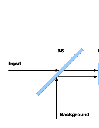
Figure 1: Model of an imperfect detector.

In the theory of quantum detection, an imperfect detector exhibiting dark counts is modeled by a compound detector, consisting of a perfect detector set in one of the outgoing arms of a beam splitter. This beam splitter mixes incoming light fields with a background radiation field (see Fig. 1). The efficiency $\eta$ of the actual detector is modeled by the transmission coefficient $|T|^{2}$ of the beam splitter. The background radiation field is assumed to be coupled to a thermal bath, and is best described as a multi-mode field.

Under the additional and well-justified assumption that the number of modes in the background field is much larger than the number of photons, coupling between background modes and incoming modes can be ignored (see, e.g. Refs. semenov and mandel p. 681). Under this assumption, the background photon distribution is approximately Poissonian. We will assume that the mean value of the number of dark counts per measurement interval is known, a value denoted by $\alpha$. Thus, the number of dark counts per measurement interval is a random variable $R\sim{\mathbb{P}}(\alpha)$.

Given this physical model, the detection statistics can be derived as follows. The conditional probability that the detector produces $m$ counts given that $n$ photons are present in the incoming field and $r$ photons in the background field is given by hong

$$f_{M|N,R}(m|n,r) = f_{M|N,R}(m-r|n,0)$$ (1)

$$= {n\choose m-r}\eta^{m-r}(1-\eta)^{n-m+r},$$

where the binomial coefficient is taken to be 0 whenever $r>m$ or $m-r>n$. Since under the given assumption the background photon distribution is approximately Poissonian, we set $R\sim{\mathbb{P}}(\alpha)$ and obtain

$$f_{M|N}(m|n)=e^{-\alpha}\sum_{r=0}^{m}\frac{1}{r!}{n\choose m-r}\alpha^{r}\eta^{m-r}(1-\eta)^{n-m+r}.$$ (2)

For a given photon number distribution of the incoming light field, $f_{N}(n)$, the distribution of the photon counts is

$$f_{M}(m)=\sum_{n=0}^{\infty}f_{M|N}(m|n)\,f_{N}(n).$$ (3)

One verifies easily that if the incoming light field is Poissonian, $N\sim{\mathbb{P}}(\nu)$, with $f_{N}(n)=\exp(-\nu)\nu^{n}/n!$, the distribution of $M$ is Poissonian also, $M\sim{\mathbb{P}}(\alpha+\eta\nu)$, as expected.

If the incoming light field is in a Fock state, with either $n=0$ or $n=1$, the formulas reduce to

$$f_{M|N}(m,0)=e^{-\alpha}\frac{\alpha^{m}}{m!}$$ (4)

for $n=0$ (no input photon), and

$$f_{M|N}(m,1)=e^{-\alpha}\left[(1-\eta)\frac{\alpha^{m}}{m!}+\eta\frac{\alpha^{m-1}}{(m-1)!}\right]$$ (5)

for $n=1$ (single input photon). With short laser pulses, one usually only wants to discriminate between $m=0$ and $m\neq 0$ (let alone that further discrimination is at all possible). Hence one is only interested in

$$f_{M|N}(0,0)=e^{-\alpha},$$ (6)

(no click, no input photon), and

$$f_{M|N}(0,1)=e^{-\alpha}(1-\eta),$$ (7)

(no click, 1 input photon), and their complementary values. Usually, $\alpha$ is rather small, and one can set $e^{-\alpha}\approx 1-\alpha$.

III Single Photon Pulses

In this section we treat the case of a pulsed laser beam, where each pulse consists of a single photon. The statistics of the detection events are governed by the binomial or multinomial distribution. We treat three different setups. First, a 2-outcome POVM where only one detector is used; the second detector, for the second outcome, is left out on the assumption that the total number of detection events should be equal to the number of pulses anyway. For perfect detectors, this assumption is correct, while in the presence of detector imperfections this is only an approximation. We will study how this affects the detection statistics. Next, we treat a 2-outcome POVM with both detectors in use and compare it with the previous case. Finally, a $K$-outcome POVM is considered, generalising the $K=2$ case.

III.1 Single Detector

We first consider the most simple case of a 2-outcome POVM where only one detector is used. The tomographic apparatus, apart from the detectors, is hereby treated as a black box with $2$ output terminals, one for each POVM element, and we assume that in each of the $N$ runs, for a fixed setting of the POVM, a single photon appears at one of the output terminals. Losses in the tomographic apparatus itself are disregarded, because that is inessential for the derivation of the detector model. The tomography black box can thus be modeled by a $2$-dimensional probability distribution $\bm{p}=(p,1-p)$, where $p$ represents the probability that the photon appears at terminal $1$ (see Fig. 2).

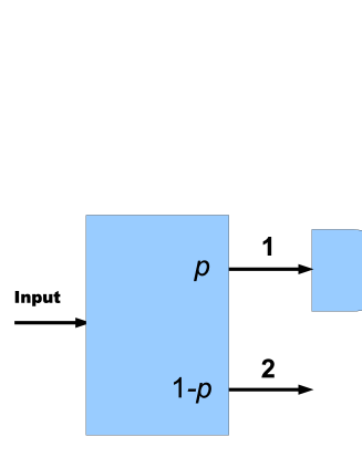
Figure 2: Model of a 2-outcome POVM where only one detector is used.

Terminal 1 is then connected to a detector with dark count rate $\alpha$ and efficiency $\eta$, while terminal 2 is left open; this corresponds to the cheapest implementation of a 2-outcome detector. The record of an $N$-run experiment consists of the number of times $g$ the detector has clicked.

III.1.1 Statistical model

We first derive the statistical properties of the random variable $G$, whose observations are the recorded photon count $g$. Its distribution is conditional on $P$ and depends on the parameters $\alpha$ and $\eta$. The standard procedure is to first derive the conditional probabilities of a detector clicking or not clicking conditional on a photon coming in or not. These are given by (cf. Sec. II):

$$\mbox{Pr}(1|0) = \mbox{Pr}(\text{click}|\text{no photon})=\alpha,$$

$$\mbox{Pr}(0|0) = \mbox{Pr}(\text{no click}|\text{no photon})=1-\alpha,$$

$$\mbox{Pr}(0|1) = \mbox{Pr}(\text{no click}|\text{photon})=\beta,$$

$$\mbox{Pr}(1|1) = \mbox{Pr}(\text{click}|\text{photon})=1-\beta.$$ (8)

Here we have introduced the attenuation factor $\beta$ as

$$\beta:=(1-\alpha)(1-\eta).$$ (9)

Using these conditional probabilities we can calculate the probability $q$ that the detector clicks:

$$q := \mbox{Pr}(\text{click})$$

$$= \mbox{Pr}(\text{click}|\text{no photon})\mbox{Pr}(\text{no photon})$$

$$\mbox{}+\mbox{Pr}(\text{click}|\text{photon})\mbox{Pr}(\text{photon})$$

$$= \alpha(1-p)+(1-\beta)p$$

$$= \alpha+(1-\alpha-\beta)p$$

$$= \alpha+\gamma p,$$

where in the last line we defined $\gamma$ as the slope of the $q$ versus $p$ curve, $\gamma:=1-\alpha-\beta=(1-\alpha)\eta$.

From this probability, one directly obtains the probability that in $N$ runs $g$ clicks are counted given the probability $p$ of an incoming photon. Obviously, $g$ should be an integer between 0 and $N$. The conditional probability distribution of the count $G$, conditional on $P$, is just the binomial distribution $\text{Bin}(N;q)$ with probability distribution function (PDF)

$$f_{G|P}(g|p)={N\choose g}\,q^{g}(1-q)^{N-g}.$$ (10)

III.1.2 Statistical Inference

From the general formula (10) describing the statistical behaviour of an imperfect detector we can derive the likelihood function $L_{P|G}$ that is needed for the Bayesian inference procedure. It is immediately clear from Eq. (10) that the likelihood function of $\alpha+(1-\alpha-\beta)P$ will be proportional to the PDF of a beta-distribution with parameters $a=g+1$ and $b=N-g+1$. To that we can add some prior information: $P$ is restricted to the interval $[0,1]$. This implies that the beta-distribution of $\alpha+\gamma P$ will have to be truncated to the interval $[\alpha,1-\beta]$.

The moments of this truncated beta-distribution are given by (with ${\mathbb{E}}[X]$ denoting the expectation value of a random variable $X$)

$$m_{1} := {\mathbb{E}}[\alpha+\gamma P]$$ (11)

$$= \frac{B(\alpha,1-\beta,g+2,N-g+1)}{B(\alpha,1-\beta,g+1,N-g+1)},$$

$$m_{2} := {\mathbb{E}}[(\alpha+\gamma P)^{2}]$$ (12)

$$= \frac{B(\alpha,1-\beta,g+3,N-g+1)}{B(\alpha,1-\beta,g+1,N-g+1)}.$$

Here, $B(x_{0},x_{1},a,b)$ is the generalised incomplete beta function. In actual numerical computations, it is better to use the regularised incomplete beta function $I_{x_{0},x_{1}}(a,b)$. Exploiting the relation $B(a+1,b)/B(a,b)=a/(a+b)$, we then get

$$m_{1} = \frac{I_{\alpha,1-\beta}(g+2,N-g+1)}{I_{\alpha,1-\beta}(g+1,N-g+1)}\,\,m_{1,0},$$ (13)

$$m_{2} = \frac{I_{\alpha,1-\beta}(g+3,N-g+1)}{I_{\alpha,1-\beta}(g+1,N-g+1)}\,\,m_{2,0},$$ (14)

$$m_{1,0} = \frac{g+1}{N+2},$$ (15)

$$m_{2,0} = \frac{(g+1)(g+2)}{(N+2)(N+3)},$$ (16)

where the first factor in Eqs. (13) and (14) is a correction term that goes to 1 when $\alpha$ and $\beta$ tend to 0, that is, for ideal detectors. From these expressions, the central moments of $P$ can then be calculated as

$$\mu(P|G=g) = \frac{m_{1}-\alpha}{1-\alpha-\beta},$$ (17)

$$\sigma^{2}(P|G=g) = \frac{m_{2}-m_{1}^{2}}{(1-\alpha-\beta)^{2}}.$$ (18)

Figure 3 shows a plot of $\mu$ [Eq. (17)] as a function of $g/N$ for a few values of $N$. As could be expected, for sufficiently large $N$, the curve for $\mu$ approaches a piecewise linear curve with $\mu=0$ for $0\leq g/N\leq\alpha$, and $\mu=1$ for $1-\beta\leq g/N\leq 1$.

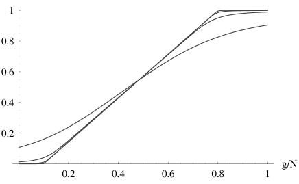
Figure 3: Plot of $\mu(P|G=g)$ [Eq. (17)] as a function of $g/N$ for $N=10$, $100$, $1000$, and $10000$, and values of $\alpha=0.1$ and $\beta=0.2$.

Figure 4 singles out the case $N=100$ and depicts the values of the first and second central moments, $\mu$ and $\sigma$.

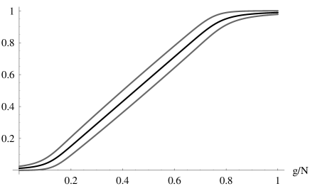
Figure 4: Plot of $\mu(P|G=g)$ [Eq. (17)] (black, central curve) and $\sigma(P|G=g)$ [Eq. (18)] (depicted as the grey curves $\mu\pm\sigma$) as a function of $g/N$ for $N=100$ and values of $\alpha=0.1$ and $\beta=0.2$.

III.1.3 Discussion

A common way to deal with dark counts and non-unit detector efficiency is to subtract the dark count rate $\alpha$ from the relative count frequencies $g/N$, replacing negative numbers by 0 if necessary, and then divide by $1-\alpha-\beta$, replacing numbers higher than 1 by 1, if necessary. In other words, one would use formula (17) with $g/N$ in place of $m_{1}$, and truncate the outcome to the interval $[0,1]$.

We argue that there are two distinct problems with this approach. First, as we have already argued in Ref. kalman1 , for given $g$, the inferred distribution of $P$ is a beta (Dirichlet) distribution, not a binomial (multinomial) distribution. Considering the extremal case $g/N\leq\alpha$, the above method would assign 0 to the probability $P$, which amounts to claiming that the outcome can never happen (except for dark counts). Of course, never having seen an event does not imply that the event is impossible. Indeed, the correct approach, using the beta distribution, assigns non-zero mean and variance to $P$. Second, as can be seen from Figs. 3 and 4, the actual behaviour of the statistically correct inferences for $P$ vary smoothly with $g$ and the truncation mentioned above is only correct in the $N\to\infty$ limit.

III.2 A $2$-outcome experiment with $2$ detectors

In this Section, we consider the situation where a single photon can take one of two paths (with probability $p$ and $1-p$, respectively), and subsequently impinges on one of two detectors, each set along one path (Fig. 5).

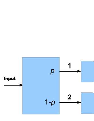
Figure 5: Model of a 2-outcome POVM where 2 detectors are used.

III.2.1 Statistical Model

Let detector $i$ be characterised by a dark rate $\alpha_{i}$ and an attenuation factor $\beta_{i}$. Concerning the presence of the photon at the detectors, there are two exclusive events: event $10$, where the photon is at detector $1$ and not at detector $2$, or event $01$, where the photon is at detector 2 instead. Concerning the detectors clicking, there are 4 events: $00$, $10$, $01$ and $11$, corresponding to no detector clicking, only detector 1 clicks, only detector 2 clicks, or both detectors are clicking. We stress again that we are considering single-photon experiments, hence the latter case of both detectors clicking would typically correspond to one detector detecting the photon just mentioned while the other detector is producing a dark count. With perfect detectors such an event would not occur.

The corresponding conditional probabilities are easily calculated. Let $\mbox{Pr}(ij|kl)$ denote this conditional probability, where $i=1$ iff detector 1 clicks, $j=1$ iff detector 2 clicks, $k=1$ iff a photon is at detector 1, and $l=1$ iff a photon is at detector 2; hence, $k+l=1$. Because the two detectors are independent, we have $\mbox{Pr}(ij|kl)=\mbox{Pr}(i|k)\,\mbox{Pr}(j|l)$, where $\mbox{Pr}(\cdot|\cdot)$ is the single-detector conditional probability (8) of the previous section.

Combined with the probability of the photon events $10$ and $01$ being $\mbox{Pr}(k=1)=p$ and $\mbox{Pr}(l=1)=1-p$, this gives the probabilities of the click events:

$$q_{00} = p\beta_{1}(1-\alpha_{2})+(1-p)(1-\alpha_{1})\beta_{2},$$ (19)

$$q_{01} = p\beta_{1}\alpha_{2}+(1-p)(1-\alpha_{1})(1-\beta_{2}),$$ (20)

$$q_{10} = p(1-\beta_{1})(1-\alpha_{2})+(1-p)\alpha_{1}\beta_{2},$$ (21)

$$q_{11} = p(1-\beta_{1})\alpha_{2}+(1-p)\alpha_{1}(1-\beta_{2}).$$ (22)

The probabilities of the corresponding event frequencies $g_{00}$, $g_{01}$, $g_{10}$ and $g_{11}$, counting over $N$ runs, is given by the multinomial distribution

$$f_{\bm{G}|P}={N\choose g_{00},g_{01},g_{10},g_{11}}q_{00}^{g_{00}}q_{01}^{g_{01}}q_{10}^{g_{10}}q_{11}^{g_{11}}.$$ (23)

Note that if one does not distinguish between single click events and two-click events, one is capturing the sums $g_{01}+g_{11}$ and $g_{10}+g_{11}$, in which the 2-click events are counted twice. This causes mathematical difficulties in the statistical inference process that are best avoided.

One may actually discard the multiple-click events altogether, and only record the single-click events $g_{1}:=g_{10}$ and $g_{2}:=g_{01}$. This means that one makes no distinction between $g_{00}$ and $g_{11}$. The corresponding distribution is again multinomial, but now given by

$$f_{G_{1},G_{2}|P}={N\choose g_{1},g_{2},g_{0}}q_{10}^{g_{1}}q_{01}^{g_{2}}(q_{00}+q_{11})^{g_{0}}.$$ (24)

with $g_{0}=N-g_{1}-g_{2}$.

In the special case that both detectors are identical, i.e. when they have the same dark count rates and attenuation factors, $\alpha_{1}=\alpha_{2}=\alpha$, and $\beta_{1}=\beta_{2}=\beta$, we find that the third factor $q_{00}+q_{11}$ reduces to the constant $\beta(1-\alpha)+\alpha(1-\beta)$, independent of $p$. Then, considered as a function of $p$, $f_{G_{1},G_{2}|P}$ is proportional to the binomial PDF ${g_{1}+g_{2}\choose g_{1}}q_{10}^{g_{1}}q_{01}^{g_{2}}$, with

$$q_{10} = (1-p)\alpha\beta+p(1-\alpha)(1-\beta),$$ (25)

$$q_{01} = p\alpha\beta+(1-p)(1-\alpha)(1-\beta).$$ (26)

Defining

$$a_{1} := \alpha\beta,$$ (27)

$$a_{2} := (1-\alpha)(1-\beta),$$ (28)

we have $q_{10}=a_{1}+(a_{2}-a_{1})p$ and $q_{01}=a_{2}-(a_{2}-a_{1})p$. Furthermore, by defining

$$a:=\frac{a_{1}}{a_{1}+a_{2}},$$ (29)

we find that $q_{10}=(a_{1}+a_{2})[a+(1-2a)p]$ and $q_{01}=(a_{1}+a_{2})[a+(1-2a)(1-p)]$.

Thus, the PDF $f_{G_{1},G_{2}|P}$ is proportional to the truncated binomial PDF:

$$f_{G_{1},G_{2}|P}\propto{g_{1}+g_{2}\choose g_{1}}[a+(1-2a)p]^{g_{1}}[a+(1-2a)(1-p)]^{g_{2}}.$$ (30)

This PDF is essentially identical to the PDF (10) obtained in the previous section, apart from the fact that the dark count rate $\alpha$ and the attenuation factor $\beta$ only enter in the PDF via the single constant $a$. This constant assumes the role of an effective dark count rate and is given by

$$a=\frac{a_{1}}{a_{1}+a_{2}}=\frac{\alpha\beta}{(1-\alpha)(1-\beta)+\alpha\beta}.$$ (31)

One sees that $a$ is of the order of $\alpha\beta$, which is a smaller number than $\alpha$ and $\beta$. More precisely, we have $\alpha\beta\leq a\leq 2\alpha\beta$.

III.2.2 Statistical Inference

In general, the statistical inference formulas become quite complicated, because in the expression for $f_{G_{1},G_{2}|P}$ more than 2 factors appear that have a dependence on $p$. The subsequent integrals over $p$ can no longer be expressed as (incomplete) beta functions. In this section we treat the easiest case of all detectors being equal, and use the PDF (30), which only has two factors. As this PDF is essentially identical to the PDF (10) obtained in the previous section, the same results therefore hold for the statistical inference.

We can therefore use formulas (13)–(18), provided we perform the substitutions $g\to g_{1}$, $N\to g_{1}+g_{2}$, $\alpha\to a$ and $\beta\to a$. This gives

$$m_{1}(a) = \frac{I_{a,1-a}(g_{1}+2,g_{2}+1)}{I_{a,1-a}(g_{1}+1,g_{2}+1)}\,\,m_{1,0},$$ (32)

$$m_{2}(a) = \frac{I_{a,1-a}(g_{1}+3,g_{2}+1)}{I_{a,1-a}(g_{1}+1,g_{2}+1)}\,\,m_{2,0},$$ (33)

$$m_{1,0} = \frac{g_{1}+1}{g_{1}+g_{2}+2},$$ (34)

$$m_{2,0} = \frac{(g_{1}+1)(g_{1}+2)}{(g_{1}+g_{2}+2)(g_{1}+g_{2}+3)}$$ (35)

and

$$\mu(P|G=(g_{1},g_{2})) = \frac{m_{1}-a}{1-2a},$$ (36)

$$\sigma^{2}(P|G=(g_{1},g_{2})) = \frac{m_{2}-m_{1}^{2}}{(1-2a)^{2}}.$$ (37)

The main difference between Eqs. (32)–(37) and Eqs. (13)–(18) for the single-detector case is the replacement of $\alpha$ and $1-\beta$ as limits of the incomplete beta functions by $a$ and $1-a$, where $a$ is the effective dark count rate given by Eq. (31).

III.2.3 Discussion

We can compare the performance of the two setups, one detector or two detectors, by comparing the average value of $\sigma$ of the reconstructed distribution of $p$, for a given value of the actual $p$. In the 1-detector case, $G$ is distributed according to Eq. (10). For given actual $p$, one calculates the average of $\sigma$ as given by Eq. (18) over this distribution. In the 2-detector case, $G_{1},G_{2}$ are distributed according to Eq. (30), and one similarly calculates the average of $\sigma$ as given by Eq. (37). Taking, as in Fig. 3, $\alpha=0.1$, $\beta=0.2$ and $N=100$, we find, for various settings of the actual $p$, the values collected in Tab. 1.

$p$	$\sigma$(1-detector)	$\sigma$(2-detectors)
0	0.033	0.044
0.5	0.070	0.088
1	0.04	0.044

Table 1: Average values for $\sigma$ for various settings of $p$, comparing the 1-detector and 2-detector cases.

It emerges that the one-detector case performs slightly better on average. Presumably, this is because for the 2-detector case we only used single click events to keep the inference procedure simple. That is, the sum $g_{1}+g_{2}$ is always less than $N$. With the given parameter settings, the average value of $g_{1}+g_{2}$ is 50 (for any $p$). However, if one makes more measurement runs for the 2-detector case, stopping when $g_{1}+g_{2}$ is equal to the number of runs for the 1-detector case, the 2-detector setup performs better (Tab. 2).

$p$	$\sigma$(1-detector)	$\sigma$(2-detectors)
0	0.033	0.017
0.5	0.070	0.052
1	0.04	0.017

Table 2: Average values for $\sigma$ in the 1-detector and 2-detector protocols under the additional constraint that $g_{1}+g_{2}$ equals the number of runs for the 1-detector case.

In Figs. 6 and 7 we show what happens to Figs. 3 and 4 for the 2-detector setup (under the constraint $g_{1}+g_{2}=100$). The plateaus around $\mu=0$ and $\mu=1$ are indeed much shorter. In addition, the error bars (quantified by $\sigma$) are smaller by a factor of roughly $1/\sqrt{2}$ (corresponding to an on average increase of $N$ by a factor of 2).

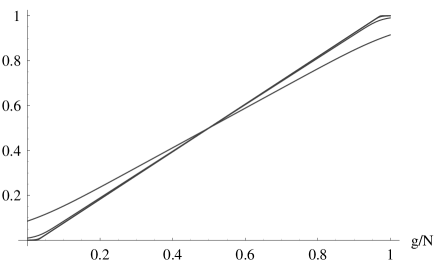
Figure 6: Plot of $\mu(P|G=(g,N-g))$ as a function of $g/N$ for $N=10$, $100$, $1000$, and $10000$, and values of $\alpha=0.1$ and $\beta=0.2$.

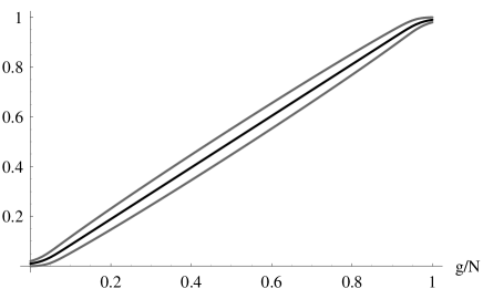
Figure 7: Plot of $\mu(P|G=(g,N-g))$ and $\sigma(P|G=(g,N-g))$ (depicted as the grey curves $\mu\pm\sigma$) as a function of $g/N$ for $N=100$ and values of $\alpha=0.1$ and $\beta=0.2$.

III.2.4 Unequal Detectors

In the more realistic case that detector parameters are not equal, we need to calculate integrals of the form

$$J(\bm{g};\bm{a},\bm{b})=\int_{0}^{1}dp\,\prod_{i}(a_{i}+b_{i}p)^{g_{i}},$$

with more than 2 factors. Indeed, the mean of $P$ can be calculated from

$$J_{1}={\mathbb{E}}[a_{1}+b_{1}P]=\frac{J(\bm{g}+\bm{e}^{1};\bm{a},\bm{b})}{J(\bm{g};\bm{a},\bm{b})},$$

and its variance from

$$J_{2}={\mathbb{E}}[(a_{1}+b_{1}P)^{2}]=\frac{J(\bm{g}+2\bm{e}^{1};\bm{a},\bm{b})}{J(\bm{g};\bm{a},\bm{b})},$$

where $\bm{e}^{i}$ denotes the unit vector along the $i$-th dimension, $\bm{e}^{i}=(0,\ldots,1,\ldots,0)$. Hence,

$$\mu_{P} = (J_{1}-a_{1})/b_{1},$$

$$\sigma^{2}_{P} = (J_{2}-a_{1}^{2}-2a_{1}b_{1}\mu_{P})/b_{1}^{2}-\mu_{P}^{2}.$$

The actual integrations can be performed numerically using standard quadrature methods (e.g. Matlab’s built-in quadl routine).

To enhance numerical robustness for higher values of $N=\sum_{i}g_{i}$, for which the integrand is sharply peaked, it is advisable to reduce the integration interval and only integrate over that subinterval of $[0,1]$ where the integrand is higher than, say, $10^{-6}$ times its maximal value. This refinement allows the quadrature algorithm to better place its quadrature points.

III.3 A $K$-outcome POVM with $K$ Detectors

Here, we generalise the results of Sec. III.2 to the case where there are $K$ detectors, each one corresponding to one of the outcomes. No detector is missing. The tomographic apparatus is now treated as a black box with $K$ output terminals, one for each POVM element. To keep the calculations for the statistical inference transparent, we restrict ourselves to the case of identical detectors throughout.

III.3.1 Statistical Model

Again we assume that in each of the $N$ runs, for a fixed setting of the POVM, a single photon appears at one of the output terminals. The tomography black box is now modeled by a $K$-dimensional probability distribution $\bm{p}=(p_{k})_{k=1}^{K}$, where $p_{k}$ represents the probability that the photon appears at terminal $k$.

Each terminal is then connected to a detector with dark count rate $\alpha$, efficiency $\eta$, and attenuation factor $\beta$. The record of an $N$-run experiment consists of the frequencies $g_{k}$, $k=1,\ldots,K$, the number of times the $k$-th detector has clicked and none of the others has. As discussed before, we leave out events where more than one detector clicked, in order not to increase the mathematical complexity.

We now derive the statistical properties of the vector $\bm{G}=(G_{k})_{k=1}^{K}$, whose observations are the recorded photon counts $\bm{g}$. Its distribution is conditional on the probability vector $\bm{p}$ and depends on the parameters $\alpha$ and $\beta$.

Let $q_{k}$ denote the probability of the event $E_{k}$ that detector $k$ clicks and no other. We again first calculate the conditional probabilities of $E_{k}$, conditional on the photon appearing at terminal $j$. For $j=k$, this conditional probability is $(1-\alpha)^{K-1}(1-\beta)$; for $j\neq k$ it is $\alpha\beta(1-\alpha)^{K-2}$.

The probability of event $E_{k}$ is then given by

$$q_{k} = (1-\alpha)^{K-2}[(1-\alpha)(1-\beta)p_{k}+\alpha\beta(1-p_{k})]$$ (38)

$$= \frac{a_{1}+(a_{2}-a_{1})p_{k}}{(K-1)a_{1}+a_{2}}$$

$$= a+(1-Ka)p_{k},$$

where $a_{1}$ and $a_{2}$ are defined as before, and the effective dark count rate $a$ is defined as

$$a:=\frac{a_{1}}{(K-1)a_{1}+a_{2}}.$$ (39)

For the $N$-run experiment, the probability of the vector of frequencies $\bm{g}=(g_{1},g_{2},\ldots,g_{K})$ is therefore proportional to the truncated multinomial distribution

$$f_{\bm{G}|\bm{P}}(\bm{g}|\bm{p})\propto{\sum_{k}g_{k}\choose g_{1},\ldots,g_{K}}\prod_{i=1}^{K}[a+(1-Ka)p_{i}]^{g_{i}}.$$ (40)

III.3.2 Statistical Inference

From the general formula (40) describing the statistical behaviour of a bank of imperfect detectors we immediately derive that the likelihood function $L_{\bm{P}|\bm{G}}$ is given by

$$L_{\bm{P}|\bm{G}}=\frac{1}{{\mathcal{N}}}\,\prod_{i=1}^{K}[a+(1-Ka)p_{i}]^{g_{i}},$$ (41)

where ${\mathcal{N}}$ is the normalisation integral, given by the integral of $[a+(1-Ka)p_{1}]^{g_{1}}\ldots[a+(1-Ka)p_{K}]^{g_{K}}$ over the probability simplex $p_{k}\geq 0$, $\sum_{k}p_{k}=1$. This integral is quite hard to calculate, and so are the integrals that are required to calculate the moments of $L_{\bm{P}|\bm{G}}$. Denoting

$$r_{k}:=a+(1-Ka)p_{k},$$ (42)

we get that the random vector $\bm{R}=(R_{1},\ldots,R_{K})$ is distributed according to a truncated Dirichlet distribution, where $R_{k}$ is subject to the condition $R_{k}\geq a$.

No analytic expression is known for the integrals involved; among the numerical methods to calculate them are numerical integration, the Gibbs sampling method (a Monte Carlo method) boyer07 , and saddle-point approximations walrus . Since for neither method commonly available software seems to exist, we give some more details about the latter method in Appendix A, where we calculate the normalisation integral of the truncated Dirichlet distribution

$$J(\bm{\alpha};a):=P(\bm{R}\geq a)=\int_{\genfrac{}{}{0.0pt}{}{r_{i}\geq a}{\sum_{i}r_{i}=1}}d\bm{r}f_{\bm{R}}(\bm{r}),$$

for $\bm{R}\sim\mbox{Dir}(\bm{\alpha})$, where as usual $\bm{\alpha}=\bm{g}+1$. The first and second order moments about the origin of $\bm{R}$ can be expressed in terms of this integral as

$${\mathbb{E}}[R_{i}] = \frac{J(\bm{\alpha}+\bm{e}^{i};a)}{J(\bm{\alpha};a)}\,\frac{\alpha_{i}}{\alpha_{0}}$$ (43)

$${\mathbb{E}}[R_{i}^{2}] = \frac{J(\bm{\alpha}+2\bm{e}^{i};a)}{J(\bm{\alpha};a)}\,\frac{\alpha_{i}(\alpha_{i}+1)}{\alpha_{0}(\alpha_{0}+1)}$$ (44)

$${\mathbb{E}}[R_{i}R_{j}] = \frac{J(\bm{\alpha}+\bm{e}^{i}+\bm{e}^{j};a)}{J(\bm{\alpha};a)}\,\frac{\alpha_{i}\alpha_{j}}{\alpha_{0}(\alpha_{0}+1)}.$$ (45)

The moments of $\bm{P}$ then follow easily from Eq. (42).

Note, however, that this calculation requires $K+1+K(K+1)/2$ separate integrations, which can be computationally very expensive for larger values of $K$. For relatively small values of $a$, say $a<0.1$, the following provides a moderately good approximation:

$$J(\bm{\alpha};a)\approx\prod_{i=1}^{K}I_{1-a}(\alpha_{0}-\alpha_{i},\alpha_{i})$$ (46)

with $I_{1-a}(\alpha_{0}-\alpha_{i},\alpha_{i})$ the regularised incomplete beta function [see Eq. (79)]. Numerical experiments indicate that this approximation is good enough for the calculation of the second order moments of $\bm{R}$ for values of $a$ as large as $0.1$. This has been checked for $K=3$; with $a=0.1$, the approximated second order moment differs less than 5% from its actual value. Similarly, the first order moments are accurate to within $0.1\sigma$ for $a\leq 0.05$.

The worst case figures appear for extremal values of $\bm{G}$, i.e. all $g_{i}=0$ bar one. Although the relative error for these extremal values increases with $N$, in practice however, these extremal values will hardly ever occur, exactly because of the presence of dark counts, as indicated by $a$. Therefore, given $a$ and $N$, we first find the minimal value of the $g_{i}$ that can sensibly occur and then calculate the relative error for that point. Since $\bm{G}$ is distributed as a truncated multinomial one should take $g_{i}\geq Na-2\sqrt{Na(1-a)}$. The relative error for points within these boundaries is then less than $0.1\sigma$, independently of $N$.

We have compared the speed of three methods to calculate/approximate the moments of $\bm{P}$. The calculations have been done in Matlab, with the routines for the incomplete beta and incomplete gamma function replaced by proprietary C implementations (available from extra ). Method 1 is the saddle-point method combined with one numerical integration (see appendix), method 2 is the saddle-point method combined with analytical integration of a Taylor series approximation (see appendix), and method 3 uses approximation (46). For $K=3$, $a=0.1$ and $\bm{\alpha}=[10,10,50]$, method 1 took 142ms, method 2 10ms, and method 3 1.7ms, on an Intel Core2 duo T7250 CPU running at 2GHz. Method 1 is the most accurate, and method 3 the least.

IV Dealing with Parameter Imprecision

In the previous section we have assumed that the two main parameters $\alpha$ and $\beta$ (dark count rate and attenuation factor) are known exactly. In realistic situations, however, $\alpha$ and $\beta$ are also of a statistical nature, for a variety of possible reasons, including instability of the parameter (drift), imprecision of the measurement of the parameter, or plain infeasibility of direct measurement. The second best thing to an accurate value for a parameter is then a statistical description in terms of a PDF or, at the very least, in terms of its mean and central moments (variance, and maybe even the skewness).

In this section we show how this statistical uncertainty about the parameters can be included in the inference process. For simplicity of the exposition, we will assume that only one parameter exhibits imprecision. The general case follows easily.

Suppose, as usual, that we want to obtain an estimate of the random variable $P$ and of its variance from measurements of $\bm{G}$, using the likelihood function $L_{P|\bm{G},Y}(p|\bm{g},y)$, where $y$ is a parameter that is described by a random variable $Y$, with given mean $\mu$, variance $\sigma^{2}$ and possibly higher order moments.

We will assume that the PDF of $Y$ is close to normal, namely continuous, single mode, small skewness and kurtosis close to the normal value of 3. Almost all of the probability mass of $Y$ is then contained in the interval $[\mu-3\sigma,\mu+3\sigma]$. PDFs of this kind can be well approximated by a so-called Edgeworth expansion hall ; blinnikov . A second order Edgeworth PDF is just the normal PDF with the given mean and variance:

$$f_{Y,2}(y)=\frac{1}{\sqrt{2\pi}\sigma}\,\exp[-(y-\mu)^{2}/2\sigma^{2}].$$

A third order Edgeworth PDF adds another term, which contains the skewness $\gamma$. For a standardised random variable (zero-mean and unit variance) this PDF reads

$$f_{Y,3}(y)=\phi(y)-\frac{\gamma}{6}\phi^{\prime\prime\prime}(y)=[1-\gamma(3-y^{2})y/6]\phi(y),$$

where $\phi$ is the standardised normal PDF $\phi(y)=\exp(-y^{2}/2)/\sqrt{2\pi}$.

Recall that if $Y$ were known perfectly, we would need to calculate only the following:

$${\mathbb{E}}[P] = \frac{\int_{0}^{1}\,\mathrm{d}p\,\,p\,\,L_{P|\bm{G}}(p|\bm{g},y)}{\int_{0}^{1}\,\mathrm{d}p\,L_{P|\bm{G}}(p|\bm{g},y)},$$

$${\mathbb{E}}[P^{2}] = \frac{\int_{0}^{1}\,\mathrm{d}p\,\,p^{2}\,\,L_{P|\bm{G}}(p|\bm{g},y)}{\int_{0}^{1}\,\mathrm{d}p\,L_{P|\bm{G}}(p|\bm{g},y)},$$

i.e. 3 integrals in total. Since, however, $Y$ enters as a nuisance parameter, we must also integrate out $Y$, taking into account the PDF of $Y$. Hence we need three double integrals, which we would like to avoid for efficiency reasons.

The method we will employ to simplify these calculations is to first perform the integration over $p$ (analytically or numerically, depending on what is possible), then approximate each such integral by a polynomial of low degree (3 or 4) in $y$, (this is the idea behind the Newton-Cotes integration formulas) and finally perform the integration over $Y$ analytically, with a low-order Edgeworth PDF substituted for the PDF of $Y$.

To obtain a polynomial approximation we will use Lagrange interpolation. Let $y_{i}$ be $m$ equidistant points within the interval $[\mu-3\sigma,\mu+3\sigma]$ (with $m$ equal to 3 or 4), say $y_{i}=i\delta$, with $i=-1,0,1$ or $i=-3/2,-1/2,1/2,3/2$. Then any function $h(y)$ can be approximated by a polynomial $\hat{h}(y)$ given by Lagrange’s interpolation formula

$$\hat{h}(y)=\sum_{k}h(y_{k})\,\prod_{i,i\neq k}\frac{y-y_{i}}{y_{k}-y_{i}}.$$

The integration over $Y$ can now be done analytically, provided we choose a low-order Edgeworth PDF for $Y$. For $m=3$ (degree-3 interpolation) and choosing a normal PDF for $Y$ yields

$$\int\,\mathrm{d}y\,\,f_{Y}(y)\,\hat{h}(y)$$

$$=\frac{\sigma^{2}}{2\delta^{2}}h(y_{-1})+(1-\frac{\sigma^{2}}{\delta^{2}})h(y_{0})+\frac{\sigma^{2}}{2\delta^{2}}h(y_{1}).$$

Hence, if we set $\delta=\sigma$, this formula simplifies to

$$\int\,\mathrm{d}y\,\,f_{Y}(y)\,\hat{h}(y)=[h(\mu-\sigma)+h(\mu+\sigma)]/2.$$ (47)

Hence, only two evaluations of $h$ are needed, i.e. two integrations over $p$. As this has to be done for the numerator and denominator of ${\mathbb{E}}[P]$ and of ${\mathbb{E}}[P^{2}]$, this gives a total of 6 integrations. For example, the formula for $\mu_{P}$ becomes

$${\mathbb{E}}[P]=\frac{\int_{0}^{1}\,\mathrm{d}p\,\,p\,\,L(p|\bm{g},\mu-\sigma)+\int_{0}^{1}\,\mathrm{d}p\,\,p\,\,L(p|\bm{g},\mu+\sigma)}{\int_{0}^{1}\,\mathrm{d}p\,\,L(p|\bm{g},\mu-\sigma)+\int_{0}^{1}\,\mathrm{d}p\,\,L(p|\bm{g},\mu+\sigma)}.$$

For $m=4$ we can include the skewness $\gamma$ of $Y$ – it cancels out for $m=3$ – by choosing a third-order Edgeworth PDF for $Y$. When we put $\delta=2\sigma$, so that the whole $\pm 3\sigma$ interval is covered, we get in a similar way as before

$$\int\,\mathrm{d}y\,\,f_{Y}(y)\,\hat{h}(y)$$ (48)

$$= -\frac{\gamma}{48}h(\mu-3\sigma)+(\frac{1}{2}+\frac{\gamma}{16})h(\mu-\sigma)$$

$$+(\frac{1}{2}-\frac{\gamma}{16})h(\mu+\sigma)+\frac{\gamma}{48}h(\mu+3\sigma).$$

This now involves 4 evaluations of $h$, hence 4 integrals over $p$.

As a final remark, note that one can place bounds on the values of a parameter from the measurement statistics. To illustrate this, consider a run of $N$ 2-outcome pulsed experiments, with unknown dark count rate, where the number $g$ of outcomes ‘1’ is very low compared to $N$. Intuition has it that the dark count rate must be small accordingly. The likelihood function for $P$ is (see Sec. III.2)

$$L_{P}={N\choose g}[a+(1-2a)p]^{g}[a+(1-2a)(1-p)]^{N-g},$$

with effective dark count rate $a$. Since $g$ is small, this places an upper bound on the value of $a$. In effect, $a$ has to be described by a random variable, and $L_{P}$ contains that random variable. By integrating out $P$ from $L_{P}$, we obtain a distribution for $a$. The exact result is that the PDF of $a$ is proportional to

$$f(a) \propto \int_{0}^{1}\,\mathrm{d}p\,[a+(1-2a)p]^{g}[a+(1-2a)(1-p)]^{N-g}$$

$$= \frac{1}{1-2a}\int_{a}^{1-a}\,\mathrm{d}x\,x^{g}(1-x)^{N-g}$$

$$= \frac{B(a,1-a,g+1,N-g+1)}{1-2a}.$$

Rather than using the exact result here, one notes that the integrand of the second integral is proportional to the PDF of a beta distribution and therefore $f(a)$ is essentially the cumulative distribution function (CDF) of the complementary beta distribution, a function decreasing with $a$. The PDF has mean value $\mu=(g+1)/(N+2)$ and variance $\sigma^{2}=(g+1)(N+1-g)/(N+2)^{2}(N+3)$. Thus, $f(a)$ will be significant only for values of $a$ below $\mu+3\sigma$. For small $g$ and large $N$, we therefore get the promised upper bound on $a$:

$$a\leq(g+1+3\sqrt{g+1})/N.$$ (49)

V Poissonian case

In Sec. III we have treated a class of tomography experiments based on single-photon optical pulses, where the statistics of the recorded photon counts is governed by the binomial/multinomial distribution. In this section we treat continuous wave (CW) experiments. Here, the input laser beam is turned on for a fixed time $T$. The detectors are still operating in Geiger mode, and the intensity of the laser beam is such that individual photons can still be discerned. Photon counts are recorded during that same time interval $T$. The statistics are now governed by the Poisson distribution.

Note that the Poisson distribution is the limiting case of the binomial distribution for the number of runs $N$ going to infinity, while the total duration $T$ and the photon rate (average number of photons expected during $T$) are kept constant. Therefore, in principle, there should be no essential difference between the statistics of this kind of experiment and those of the single-photon experiments. However, in CW experiments, the intensity of the laser beam enters as a parameter, requiring determination. While this determination is possible by performing independent measurements, a less time-consuming approach is to use the actual measurements one is interested in. This approach will be described in this section.

We will assume again that the dark count rate $\alpha$ is known exactly. The detector attenuation factor $\beta$ will not show up explicitly as it is assumed to be absorbed into the (unknown) laser beam intensity.

V.1 Statistical Model

We consider a CW experiment consisting of $K$ runs of equal time duration $T$, and constant but unknown laser intensity. In each run a different 2-outcome POVM $\{\Pi^{(i)},\mathrm{\leavevmode\hbox{\small 1\normalsize\kern-3.30002pt1}}-\Pi^{(i)}\}$ is applied, but only the counts $g_{i}$ corresponding to $\Pi^{(i)}$ are recorded, as was the case in Sec. III.1. We assume that $\sum_{i}\Pi^{(i)}=b\mathrm{\leavevmode\hbox{\small 1\normalsize\kern-3.30002pt1}}$. The general case, in which $\sum_{i}\Pi^{(i)}$ is not a multiple of 11, has been treated (without dark counts) in Ref. kalman1 . The purpose of this section is only to show how dark counts can be added to the statistical model. Non-unit detector efficiency has already been incorporated in the treatment of Ref. kalman1 implicitly, by absorbing $\eta$ in the beam intensity $A$.

As stated in Sec. II, for Poissonian input and background fields, the counts are Poissonian too, with mean value $\mu=\alpha+\eta\nu$, where $\alpha$ is the dark count rate and $\nu$ the input photon rate. For beam intensity $A$, and POVM element $\Pi^{(i)}$, we have $\nu=Ap_{i}$, thus $\mu_{i}=\alpha+\eta Ap_{i}$. Henceforth, we absorb $\eta$ into $A$, thus $\mu_{i}=\alpha+Ap_{i}$. In addition, since $\sum_{i}\Pi^{(i)}=b\mathrm{\leavevmode\hbox{\small 1\normalsize\kern-3.30002pt1}}$, we have $\sum_{i}p_{i}=b$.

As the counts $g_{i}$ are independent, and each is Poissonian with mean $\mu_{i}$, the PDF of the sequence of counts $\bm{G}=(G_{1},G_{2},\ldots,G_{K})$ is given by

$$f_{\bm{G}}(\bm{g})=\prod_{i=1}^{K}e^{-\mu_{i}}\frac{\mu_{i}^{g_{i}}}{g_{i}!}\propto e^{-Ab}\prod_{i=1}^{K}(\alpha+Ap_{i})^{g_{i}},$$

where factors have been left out that are independent of $p_{i}$ and $A$. In order to formally turn the quantities $\alpha+Ap_{i}$ into a probability distribution, we divide by their sum $\sum_{i=1}^{K}(\alpha+Ap_{i})=K\alpha+Ab$, and define

$$\frac{\alpha+Ap_{i}}{K\alpha+Ab} = y+(1-Ky)p_{i}/b,$$ (50)

$$y := \alpha/x,$$ (51)

$$x := K\alpha+Ab.$$ (52)

Then the PDF of $\bm{G}$ is proportional to

$$f_{\bm{G}}(\bm{g})\propto\frac{e^{-x}x^{N}}{\Gamma(N+1,K\alpha)}\,\,\prod_{i=1}^{K}(y+(1-Ky)p_{i}/b)^{g_{i}},$$ (53)

with $N:=\sum_{i}g_{i}$. The factor $1/\Gamma(N+1,K\alpha)$ has been included to normalise the factor $e^{-x}x^{N}$ over the interval $x\geq K\alpha$. The first factor is, indeed, the PDF of a truncated gamma distribution.

The second factor is essentially the PDF for the single-photon case, with $y$ assuming the role of the effective dark count rate. The main difference is that $y$ is now a random variable. Indeed, as the variable $A$ is an unknown, so are $x$ and $y$. In Bayesian terminology, $A$ is a nuisance parameter, and the standard Bayesian treatment is to integrate it out. That is, $f_{\bm{G}}(\bm{g})$ is multiplied by a suitable prior for $A$, and is then integrated over $A\in[0,\infty]$. The problem with this approach is that the integral cannot be carried out analytically.

In what follows, we approximate the integral, based on the assumption that the number of total counts $N=\sum_{i}g_{i}$ should be much larger than the expected total number of dark counts $K\alpha$, i.e. that the signal-to-noise ratio of the experimental data is large enough. This assumption is very reasonable given that one actually wants to obtain useful information from the data.

The main benefit of this assumption is that the truncation of $x$ can be disregarded. Indeed, as has been noted in Sec. B, the normalisation factor $\Gamma(N+1,K\alpha)$ is well approximated by $\Gamma(N+1)$ when $N\geq 1+K\alpha+3\sqrt{K\alpha}$, and similar statements hold regarding the moments of the distribution. Thus the PDF of $\bm{G}$ is proportional to

$$f_{\bm{G}}(\bm{g})\propto\frac{e^{-x}x^{N}}{N!}\,\,\prod_{i=1}^{K}[y+(1-Ky)p_{i}/b]^{g_{i}},$$ (54)

where we now allow the random variable $X$ to assume all values down to 0. The upshot is that to very good approximation, $X$ has a gamma distribution with mean (and variance) $N+1$. The integral of $f_{\bm{G}}(\bm{g})$ over $x$ is thus a convolution of ${\mathcal{L}}(\bm{g}):=\prod_{i=1}^{K}[y+(1-Ky)p_{i}/b]^{g_{i}}$, which depends on $x$ via $y=\alpha/x$, with the gamma PDF of $X$. Note also the resemblance of Eq. (54) to the corresponding Eq. (40) for the $K$-detector single photon case, which is not all too surprising.

A short calculation using the properties of $X$ reveals that the variable $Y=\alpha/X$ has mean value $\mu_{Y}=\alpha/N$ and variance $\sigma_{Y}^{2}=\alpha^{2}/N^{2}(N-1)$. As the PDF of $Y$ shows small but noticeable deviations from a normal distribution, we also need the skewness of $Y$, which turns out to be $\gamma_{Y}=4\sqrt{N-1}/(N-2)$. Recall that the skewness is defined as the third central moment of $Y$ divided by the third power of $\sigma_{Y}$; for this distribution the skewness is roughly equal to two times Pearson’s mode skewness, and can therefore be interpreted as how much the mean differs from the mode, expressed in halves of a standard deviation. For this distribution the mode of $Y$ is $\alpha/(N+2)$.

V.2 Statistical Inference

We can now invoke the methods of Secs. III.3 and IV to perform the statistical inversion of ${\mathcal{L}}(\bm{g})$ with $Y$ as an imprecise parameter with the moments just mentioned, which depend on the dark count rate $\alpha$ (assumed to be known here) and on $N=\sum_{i}g_{i}$. As regards the additional factor $1/b$ in Eq. (54), this can be taken into account by multiplying the obtained mean of $\bm{P}$, ${\mathbb{E}}[P_{i}]$, by $b$ and the second order moments about the origin, ${\mathbb{E}}[P_{i}P_{j}]$, by $b^{2}$.

Finally, we can also treat the case where the POVM elements do not add up to a multiple of the identity, i.e. when the assumption $\sum_{i}\Pi^{(i)}=b\mathrm{\leavevmode\hbox{\small 1\normalsize\kern-3.30002pt1}}$ is not satisfied. This could occur because of inaccuracies in the implementations of the POVM elements, or simply because of the choice of elements – before Ref. kalman1 it was not known that failure to meet the condition $\sum_{i}\Pi^{(i)}=b\mathrm{\leavevmode\hbox{\small 1\normalsize\kern-3.30002pt1}}$ had a severely negative impact on the ease with which statistical inferences could be made. The consequence is that the probabilities $p_{i}$ do not add up to a constant. Their sum $p_{0}:=\sum_{i=1}^{K}p_{i}$ is now a random variable, too, and has to be treated as an additional nuisance parameter. This case has been treated, for the case without dark counts, in Ref. kalman1 , Sec. 3.2.5, under the assumption that the deviation of $\sum_{i}\Pi^{(i)}$ from a scalar matrix is small. For larger deviations no accurate methods are known to us other than Monte-Carlo methods.

The formulas obtained in Ref. kalman1 carry over easily to the case with dark counts, because $b$ simply enters as a factor in the formulas for the moments of $\bm{P}$. Let $M$ and $m$ be the largest and smallest eigenvalue of $\sum_{i}\Pi^{(i)}$. The multiplication factors for ${\mathbb{E}}[P_{i}]$ and ${\mathbb{E}}[P_{i}P_{j}]$ (the moments about the origin) are now, instead of $b$ and $b^{2}$, $M\phi_{1}$ and $M\phi_{2}$, respectively, with

$$\phi_{1} = \frac{K}{K+1}\,\frac{1-(m/M)^{K+1}}{1-(m/M)^{K}},$$ (55)

$$\phi_{2} = \frac{K}{K+2}\,\frac{1-(m/M)^{K+2}}{1-(m/M)^{K}}.$$ (56)

VI Conclusion

In this paper, we have studied the statistical properties of photon detection using imperfect detectors, exhibiting dark counts and less than unit detection efficiency, in the context of implementations of general $K$-element POVMs. We have derived a Bayesian inference procedure for obtaining distributions over outcome probabilities from detection frequencies in a variety of setups. We also obtained formulas and/or algorithms for efficiently calculating the first and second order moments of these distributions, effectively obtaining estimates and corresponding error bars for the outcome probabilities.

For experiments using single-photon laser pulses we have considered $K$-element POVMs constructed with $K$ detectors (with special emphasis on the case $K=2$). We found that by far the easiest inference procedure occurred when only taking single-detection events into account (i.e. only counting events where just one out of $K$ detector clicked). In that case, the outcome probabilities $\bm{p}$ are drawn from a truncated Dirichlet distribution $\propto\prod_{i=1}^{K}[a+(1-Ka)p_{i}]^{g_{i}}$ where $g_{i}$ are the detection frequencies and $a$ is an effective dark count rate, which can be calculated from the actual dark count rate and the detection efficiency. For $K=2$ the moments of this truncated Dirichlet can be calculated extremely rapidly using incomplete beta functions. For larger $K$ we have devised a number of numerical algorithms for doing so, offering the user a trade-off between accuracy and speed. For $K=2$ we also considered a setup with just a single detector, and found slightly different formulas for the distribution and its moments.

While in the above one needs to supply values for dark count rate and detector efficiency, we have also devised a method for dealing with the case when these parameters are not accurately known. This method is particularly useful to deal with the final setup we have considered, namely when the experiments are done with continuous wave laser beams. In that case, the detection statistics is Poissonian and the inferred outcome probabilities are again drawn from a truncated Dirichlet, but now with the effective dark count rate being a random variate itself, due to the inaccurately unknown laser beam intensity.

Finally, we also briefly considered how one can obtain an upper bound on the effective dark count rate, from the value of the minimal frequency of an outcome in any given run (or in a combination of runs).

Appendix A Integrals of truncated Dirichlet distributions

In order to calculate the moments of the truncated Dirichlet distribution, one must be able to accurately calculate the distribution’s normalisation integrals. In this Appendix, we describe an approximation method due to Butler and Sutton walrus .

Let $\bm{X}\sim\mbox{Dir}(\bm{\alpha})$ be a Dirichlet distributed $K$-dimensional random variable, with parameters $\bm{\alpha}=(\alpha_{1},\ldots,\alpha_{K})$. This assumes that $X_{i}\geq 0$ and $\sum_{i=1}^{K}X_{i}=1$ hold. We will use the common notation $\alpha_{0}=\sum_{i}\alpha_{i}$.

Let us now truncate $\bm{X}$, by imposing the condition $X_{i}\geq a$, where $0\leq a\leq 1/K$. The goal is to calculate the new integration constant given by the probability $\mbox{Pr}(\bm{X}\geq a)$. We will denote this probability integral by $J$:

$$J(\bm{\alpha};a)=\int_{\genfrac{}{}{0.0pt}{}{x_{i}\geq a}{\sum_{i}x_{i}=1}}d\bm{x}\,\,\Gamma(\alpha_{0})\,\,\prod_{i=1}^{K}\frac{x_{i}^{\alpha_{i}-1}}{\Gamma(\alpha_{i})}.$$ (57)

Note that for $K=2$, this integral is given by the regularised incomplete beta function $I_{a,1-a}(a_{1},a_{2})$.

The method proposed by Butler and Sutton consists of two basic ideas. The first idea is to use a conditional characterisation of $\bm{X}$. Namely, one defines $K$ new, independent random variables $Z_{i}$ such that $\bm{X}$ and $\bm{Z}|\sum_{i}Z_{i}=1$ have the same distribution. It is known that one obtains the required Dirichlet distribution if $Z_{i}$ has a gamma distribution, $Z_{i}\sim\mbox{Gamma}(\alpha_{i},1)$. For the purposes of the method, the value of the scale parameter $\theta$ does not matter, and we set $\theta=1$. The PDF is therefore given by

$$f_{Z_{i}}(z)=\frac{z^{\alpha_{i}-1}e^{-z}}{\Gamma(\alpha_{i})}.$$

Now the required probability $\mbox{Pr}(\bm{X}\geq a)$ can be expressed, using Bayes’ rule, as

$$\mbox{Pr}(\bm{X}\geq a)=\mbox{Pr}(\bm{Z}\geq a|\sum_{i}Z_{i}=1)$$

$$= \mbox{Pr}(\sum_{i}Z_{i}=1|\bm{Z}\geq a)\prod_{i}\mbox{Pr}(Z_{i}\geq a)\frac{1}{\mbox{Pr}(\sum_{i}Z_{i}=1)}.$$

The factors $\mbox{Pr}(Z_{i}\geq a)$ are easily calculated in terms of the CDF of the gamma distribution, giving

$$\mbox{Pr}(Z_{i}\geq a)=Q(\alpha_{i},a),$$ (59)

with $Q(\alpha_{i},a)$ the regularised incomplete gamma function.

Since the $Z_{i}$ are independently gamma-distributed, $Z_{i}\sim\mbox{Gamma}(\alpha_{i},1)$, their sum is also gamma-distributed: $\sum_{i}Z_{i}\sim\mbox{Gamma}(\alpha_{0},1)$. The factor $\mbox{Pr}(\sum_{i}Z_{i}=1)$ is therefore given by the value of the PDF of $\mbox{Gamma}(\alpha_{0},1)$ in 1, which gives:

$$1/\mbox{Pr}\left(\sum_{i}Z_{i}=1\right)=e\,\Gamma(\alpha_{0}).$$ (60)

The first factor in Eq. (LABEL:eq:A1), the truncated PDF $\mbox{Pr}(\sum_{i}Z_{i}=1|\bm{Z}\geq a)$, is the hardest to calculate, because it is a multi-dimensional integral, and the second idea in Butler and Sutton’s method is to convert it to an inverse Laplace integral of a univariate function, and then approximate the latter integral using a saddle-point method, as first proposed by Daniels daniels .

The method starts from the moment generating function (MGF) of the truncated random variable $T=\sum_{i}Z_{i}|Z\geq a$, defined as $M_{T}(s)={\mathbb{E}}_{T}[e^{st}]$. Since the $Z_{i}$ are independent, we have

$$M_{T}(s)=\prod_{i}{\mathbb{E}}_{T_{i}}[e^{st}],$$ (61)

where $T_{i}:=Z_{i}|Z_{i}\geq a$. A simple calculation gives

$${\mathbb{E}}_{T_{i}}[e^{st}] = \frac{\int_{a}^{\infty}dt\,\,e^{st}t^{\alpha_{i}-1}e^{-t}}{\int_{a}^{\infty}dt\,\,t^{\alpha_{i}-1}e^{-t}}$$ (62)

$$= (1-s)^{-\alpha_{i}}\frac{Q(\alpha_{i},(1-s)a)}{Q(\alpha_{i},a)},$$

which is valid for $\Re s<1$ (and we do need complex $s$). The denominators cancel with the factors $\mbox{Pr}(Z_{i}\geq a)=Q(\alpha_{i},a)$.

Since the MGF $M_{T}(-s)$ is the two-sided Laplace transform of the PDF, the PDF can be recovered from the MGF by an inverse Laplace transform:

$$f_{T}(t)=\frac{1}{2\pi i}\int_{\gamma-i\infty}^{\gamma+i\infty}M_{T}(s)e^{-st}ds,$$

where, in our case, we only need to evaluate the PDF at the point $t=1$. By expressing the MGF as the exponential of the cumulant generating function (CGF) $K_{T}(s):=\log M_{T}(s)$, the path of integration can be brought in a form that readily invites the saddle-point method for its approximate evaluation:

$$f_{T}(t)=\frac{1}{2\pi i}\int_{\gamma-i\infty}^{\gamma+i\infty}e^{K_{T}(s)-st}ds.$$ (63)

The path of integration is hereby chosen to pass through a saddle-point of the integrand, in such a way that the integrand is negligible outside its immediate neighbourhood. Daniels shows that in this case the path should be a straight line parallel to the imaginary axis and passing through the saddle-point $\hat{s}$, which is that value of $s$ for which the derivative of $K_{T}(s)-st$ w.r.t. $s$ vanishes:

$$K^{\prime}_{T}(\hat{s})=t.$$ (64)

Daniels showed that, under very general conditions, $\hat{s}$ is real. Hence, in Eq. (63), one takes $\gamma=\hat{s}$, and the path of integration is along points $s=\hat{s}+iy$.

An explicit formula for $K^{\prime}_{T}(s)$ is

$$K^{\prime}_{T}(s)=\frac{a}{u}\left[\alpha_{0}+\sum_{i}g(\alpha_{i},u)\right],$$ (65)

with $u=a(1-s)$ and $g(\alpha,u)=e^{-u}u^{\alpha_{i}}/\Gamma(\alpha_{i},u)$. One shows that $g(\alpha,u)$ is roughly approximated by $\max[0,u-(\alpha-1)]$; moreover, $g(\alpha,u)\geq\max[0,u-(\alpha-1)]$. An approximate value of $\hat{s}=1-\hat{u}/a$ is thus given by the solution of

$$\frac{u}{a}=\alpha_{0}+\sum_{i}\max[0,u-(\alpha_{i}-1)].$$ (66)

As the right-hand side is a piecewise linear function of $u$, the solution of this equation is easily found. This approximate solution can then be used as a starting value for numerically solving the exact equation

$$\frac{u}{a}=\alpha_{0}+\sum_{i}g(\alpha_{i},u).$$

Once the optimal value $\hat{s}$ has been obtained, one can go about performing the integration in Eq. (63), i.e. of

$$f_{T}(1)=\frac{1}{\pi}\int_{0}^{\infty}\Re[M_{T}(\hat{s}+iy)e^{-(\hat{s}+iy)}]dy,$$ (67)

where we have exploited the fact that the real part of the integrand is even in $y$. To obtain the highest accuracy, the integration has to be done using a numerical quadrature (e.g. using Matlab’s built-in quadl routine). The upper integration limit can be replaced by a finite value, equal to a fixed number times the approximate width of the function graph, which is roughly $1/\sqrt{K^{\prime\prime}_{T}(\hat{s})}$, where

$$K^{\prime\prime}_{T}(s)=\sum_{i}\frac{\alpha_{i}}{(1-s)^{2}\Gamma(\alpha_{i},a(1-s))^{2}}.$$

If speed is at a premium, while somewhat less precision is acceptable, one can use a finite-term Taylor expansion of $K_{T}(s)-s$, and integrate each of the resulting terms analytically. The saddle-point approximation is obtained by writing $K_{T}(s)-s$ as a Taylor series around $s=\hat{s}$:

$$K_{T}(s)-s=K_{T}(\hat{s})-\hat{s}+\sum_{j=2}^{\infty}\frac{1}{j!}K^{(j)}_{T}(\hat{s})(iy)^{j},$$

and expanding the integrand as

$$e^{K_{T}(s)-s} = e^{K_{T}(\hat{s})-\hat{s}}\,\,e^{-K^{\prime\prime}_{T}y^{2}/2}\exp\left[\sum_{j=3}^{\infty}\frac{1}{j!}K^{(j)}_{T}(iy)^{j}\right]$$

$$= e^{K_{T}(\hat{s})-\hat{s}}\,\,e^{-K^{\prime\prime}_{T}y^{2}/2}$$

$$\times\Bigg{\{}1-i\frac{K^{(3)}_{T}}{6}y^{3}+\frac{K^{(4)}_{T}}{24}y^{4}+i\frac{K^{(5)}_{T}}{120}y^{5}$$

$$+\left[-\frac{(K^{(3)}_{T})^{2}}{72}-\frac{K^{(6)}_{T}}{720}\right]y^{6}+\ldots\Bigg{\}}.$$

with each of the derivatives of $K_{T}$ evaluated in $\hat{s}$.

Figure 8: Plot of $J(\alpha_{1},\alpha_{2};0.1)$ as calculated using the second-order saddle-point method (blue, solid curve), and the absolute error, in units of $10^{-4}$ (red, dashed curve), as compared to the exact result $I_{0.1,0.9}(\alpha_{1},\alpha_{2})$. The sum $\alpha_{0}=\alpha_{1}+\alpha_{2}$ is held constant at a value of 50. The maximal absolute error here is $2.4571\times 10^{-5}$ and the maximal relative error is $2.5189\times 10^{-5}$.

Upon performing the integral $\int_{-\infty}^{+\infty}dy$ the terms with odd powers of $y$ vanish. After substituting $K^{\prime\prime}_{T}y^{2}/2=v^{2}$, and using

$$\int_{-\infty}^{+\infty}e^{-v^{2}}v^{2k}dv=\Gamma(k+1/2),$$

with $\Gamma(1/2)=\sqrt{\pi}$, $\Gamma(2+1/2)=3\sqrt{\pi}/4$ and $\Gamma(3+1/2)=15\sqrt{\pi}/8$, the even powers yield

$$f_{T}(1)=\frac{e^{K_{T}(\hat{s})-\hat{s}}}{\sqrt{2\pi K^{\prime\prime}_{T}}}\left(1+\frac{1}{8}\,\frac{K^{(4)}_{T}}{(K^{\prime\prime}_{T})^{2}}-\frac{5}{24}\,\frac{(K^{(3)}_{T})^{2}}{(K^{\prime\prime}_{T})^{3}}+\ldots\right),$$ (68)

(note that in the corresponding formula (7) in Ref. walrus a minus sign is missing).

In Fig. 8 we give an example of the 2-dimensional integral $J(\alpha_{1},\alpha_{2};a)$ calculated using this method and compare it to the exact result, which for $K=2$ is known to be the regularised incomplete beta function $I_{a,1-a}(\alpha_{1},\alpha_{2})$. The Matlab routines used to perform these calculations are available from extra .

Appendix B Mathematical compendium

In this appendix we gather a few mathematical preliminaries that are necessary to understand the statistical models developed in Secs. II–V.

B.1 Special functions

We start by collecting some important results on special functions and their implementations in various computer algebra software.

B.1.1 Gamma function

The gamma function $\Gamma(\alpha)$ is defined as the integral

$$\Gamma(\alpha)=\int_{0}^{\infty}\,\mathrm{d}t\,t^{\alpha-1}e^{-t}$$ (69)

with $\Gamma(k)=(k-1)!$ for integer arguments. Since for large values of its argument, the gamma function becomes extremely large, numerical packages usually contain implementations of the natural logarithm of the gamma function too (gammaln in Matlab, and LogGamma in Mathematica). We will need this as well.

The gamma integral leads to two incomplete integrals, the lower incomplete gamma function $\gamma(\alpha,x)$ and the upper incomplete gamma function $\Gamma(\alpha,x)$:

$$\gamma(\alpha,x) = \int_{0}^{x}\,\mathrm{d}t\,t^{\alpha-1}e^{-t},$$ (70)

$$\Gamma(\alpha,x) = \int_{x}^{\infty}\,\mathrm{d}t\,t^{\alpha-1}e^{-t}.$$ (71)

Obviously, one has $\gamma(\alpha,x)+\Gamma(\alpha,x)=\Gamma(\alpha)$. By dividing these incomplete gamma functions by the corresponding complete gamma, one obtains the regularised incomplete gamma functions:

$$P(\alpha,x) = \gamma(\alpha,x)/\Gamma(\alpha),$$ (72)

$$Q(\alpha,x) = \Gamma(\alpha,x)/\Gamma(\alpha),$$ (73)

with $P+Q=1$.

In Mathematica, Gamma[$\alpha$,x] is the upper incomplete gamma function $\Gamma(\alpha,x)$, while Gamma[$\alpha$,$x_{0}$,$x_{1}$] is the generalized incomplete gamma function, so that $\gamma(\alpha,x)=$ Gamma[$\alpha$,0,x]. The regularised incomplete gamma functions are implemented as $Q(\alpha,x)=$ GammaRegularized[$\alpha$,x] and $P(\alpha,x)=$ GammaRegularized[$\alpha$,0,x].

In Matlab, $P(\alpha,x)$ has been implemented as gammainc(x,$\alpha$) (note the reversal of the arguments). Except in older versions, $Q$ has been implemented too, as gammainc(x,$\alpha$,’upper’).

The two basic expansions that are used in these calculations are the series expansion (see, e.g. Ref. as , formula 6.5.29)

$$P(\alpha,x)=e^{-x}\,\sum_{k=0}^{\infty}\frac{x^{\alpha+k}}{\Gamma(\alpha+k+1)},$$

for $x<\alpha+1$, and the continued fraction expansion (see, e.g. Ref. as , formula 6.5.31)

$$Q(\alpha,x)=\frac{e^{-x}x^{\alpha}}{\Gamma(\alpha)}\left(\frac{1}{x+}\,\,\frac{1-\alpha}{1+}\,\,\frac{1}{x+}\,\,\frac{2-\alpha}{1+}\,\,\frac{2}{x+}\ldots\right),$$

for $x\geq\alpha+1$. Here we used the typographical notation for continued fractions: $\left(\frac{a}{b+}c\right)=\frac{a}{b+c}$, where $c$ stands for everything that follows. For the other regimes one can use the formula $P+Q=1$. If high accuracy is needed for extremely small values of $P$ or $Q$, one should calculate the logarithm.

B.1.2 Beta function

The beta function $B(a,b)$, a generalization of the gamma function, is defined as

$$B(a,b)=\int_{0}^{1}\,\mathrm{d}t\,t^{a-1}(1-t)^{b-1}.$$ (74)

It is related to the gamma function via

$$B(a,b)=\frac{\Gamma(a)\Gamma(b)}{\Gamma(a+b)}.$$ (75)

This leads to the relation

$$B(a+1,b)/B(a,b)=a/(a+b),$$ (76)

For integer arguments, one sees that $B(a,b)$ is related to the binomial coefficient as

$$B(a,b)=\frac{(a-1)!(b-1)!}{(a+b-1)!}=\frac{a+b}{ab{a+b\choose a}}.$$

Since, again, the natural logarithm of the beta function is usually implemented directly [in Matlab: betaln(a,b)], this formula allows evaluation of the binomial coefficients for larger values of the arguments than allowed by direct calculation.

Just as in the case of the gamma function, replacing the integration limits yields the incomplete beta function $B(x,a,b)$ and the generalised incomplete beta function $B(x_{0},x_{1},a,b)$

$$B(x,a,b) = \int_{0}^{x}\,\mathrm{d}x\,x^{a-1}(1-x)^{b-1}$$ (77)

$$B(x_{0},x_{1},a,b) = \int_{x_{0}}^{x_{1}}\,\mathrm{d}x\,x^{a-1}(1-x)^{b-1}.$$ (78)

Dividing by the complete beta function also gives the regularised incomplete beta function and the generalised regularised incomplete beta function

$$I_{x}(a,b) = B(x,a,b)/B(a,b),$$ (79)

$$I_{x_{0},x_{1}}(a,b) = B(x_{0},x_{1},a,b)/B(a,b).$$ (80)

In Matlab, only $I_{x}(a,b)=I_{0,x}(a,b)$ and $I_{x,1}(a,b)=1-I_{x}(a,b)$ are implemented, as betainc(x,a,b) and betainc(x,a,b,’upper’), the latter only in more recent versions, while in Mathematica all four functions exist, under the names Beta[x,a,b], Beta[x0,x1,a,b], BetaRegularized[x,a,b] and BetaRegularized[x0,x1,a,b]. Just as for the incomplete gamma functions one may need a logarithmic version of $I_{x}$ to cover cases with extremely small function values.

Calculations are based on the continued fraction expansion of $I_{x}$, which is valid for $x$ smaller than $(a-1)/(a+b-2)$ (see, e.g. Ref. as , formula 26.5.8):

$$I_{x}(a,b)\approx\frac{x^{a}(1-x)^{b}}{aB(a,b)}\left(\frac{1}{1+}\,\,\frac{d_{1}}{1+}\,\,\frac{d_{2}}{1+}\ldots\right)$$ (81)

with

$$d_{2m+1} = -\frac{(a+m)(a+b+m)}{(a+2m)(a+2m+1)}\,\,x,$$

$$d_{2m} = \frac{m(b-m)}{(a+2m-1)(a+2m)}\,\,x.$$

For larger $x$, one uses the relation $I_{1-x}(b,a)=1-I_{x}(a,b)$, where the left hand side is numerically more accurate for small function values. In case the continued fraction expansion fails, one can still use certain approximations (see, e.g. Ref. as , formulas 26.5.20 and 21).

B.2 Poisson, Gamma, Beta and Dirichlet Distributions

The probability distribution function (PDF) of a discrete random variable $K$ that is distributed according to the Poisson distribution, $K\sim{\mathbb{P}}(\lambda)$, is

$$f_{K}(k)=\frac{\lambda^{k}e^{-\lambda}}{k!}.$$ (82)

Its mean and variance are both equal to $\lambda$.

We also recall a number of basic facts about several continuous distributions jkb94 ; kbj . The gamma distribution is directly related to the gamma function. The PDF of a random variable $X$ that is distributed according to the gamma distribution $X\sim\mbox{Gamma}(\alpha,\theta)$, with $\alpha$ the shape parameter and $\theta$ the scale parameter, is given by

$$f_{X}(x)=\frac{e^{-x/\theta}x^{\alpha-1}}{\theta^{\alpha}\Gamma(\alpha)}.$$

We will not need the extra freedom offered by $\theta$, and we will always put $\theta=1$, giving

$$f_{X}(x)=\frac{e^{-x}x^{\alpha-1}}{\Gamma(\alpha)}.$$ (83)

For $x=\lambda$ and $\alpha=k+1$, this PDF looks formally the same as the Poisson PDF. However, in the latter $K$ is the random variable, rather than $X$. In effect, the gamma distribution and Poisson distribution are each other’s conjugate.

The cumulative distribution function (CDF) of $X$ is the regularised lower incomplete gamma function $P$:

$$\mbox{Pr}(X\geq x)=P(\alpha,x),$$ (84)

and its moments are given by

$$\mu_{X}=\sigma_{X}^{2}=\alpha.$$ (85)

For not too small values of $\alpha$, the bulk of the probability mass of the gamma distribution is roughly contained within the interval $[\mu-3\sigma,\mu+3\sigma]=[\alpha-3\sqrt{\alpha},\alpha+3\sqrt{\alpha}]$. This explains why $P(\alpha,x)$ is very close to 0 for $x\leq\alpha-3\sqrt{\alpha}$ and very close to 1 for (roughly) $x\geq\alpha+3\sqrt{\alpha}$. A more accurate statement is that for $x\geq\alpha+2.8+3.09\sqrt{\alpha}$, or $\alpha\leq x+1.9-3.09\sqrt{x-0.41}$, $P(\alpha,x)\geq 0.999$.

The Dirichlet distribution is the higher-dimensional generalisation of the beta distribution. The importance of this distribution stems from the fact that it is the conjugate distribution of the multinomial distribution: if $\bm{F}\sim\mbox{Mtn}(N,\bm{p})$ is the distribution of $\bm{F}$ conditional on $\bm{P}=\bm{p}$, then using Bayesian inversion (starting with a uniform prior for $\bm{P}$) $\bm{P}$ conditional on $\bm{F}=\bm{f}$ is Dirichlet distributed with parameter $\bm{f}$. Formally, the two distributions only differ by their normalisation. The multinomial distribution is normalised by summing over all integer non-negative $\bm{f}$ summing up to $N$, while the Dirichlet distribution is normalised by integrating over the simplex of non-negative $\bm{p}$ summing to 1.

The general form of the PDF of a $d$-dimensional Dirichlet distribution with parameters $\alpha_{i}$ is (see, e.g. Ref. kbj , Chapter 49)

$$f_{\bm{P}}(\bm{p})=\Gamma(\alpha_{0})\prod_{i=1}^{d}\frac{p_{i}^{\alpha_{i}-1}}{\Gamma(\alpha_{i})},$$

where $\alpha_{0}$ is defined as

$$\alpha_{0}:=\sum_{i=1}^{d}\alpha_{i}.$$ (86)

The range of $\bm{P}$ is the simplex $p_{i}\geq 0,\sum p_{i}=1$.

The mean values of the Dirichlet distribution are

$$\mu_{i}=\frac{\alpha_{i}}{\alpha_{0}},$$ (87)

and the elements of its covariance matrix are

$$\sigma_{ij}^{2}=\left\{\begin{array}[]{ll}\frac{\alpha_{i}(\alpha_{0}-\alpha_{i})}{\alpha_{0}^{2}(\alpha_{0}+1)},&i=j\\[5.69054pt] \frac{-\alpha_{i}\alpha_{j}}{\alpha_{0}^{2}(\alpha_{0}+1)},&i\neq j\end{array}\right..$$ (88)

The beta distribution is the special case of a Dirichlet distribution with $d=2$. The normalisation factor is then the beta function $B(\alpha_{1},\alpha_{2})$, from which the distribution got its name.

References

- (1) K.M.R. Audenaert and S. Scheel, New J. Phys. 11, 023028 (2009).
- (2) N.L. Johnson, S. Kotz, and N. Balakrishnan, Continuous Univariate Distributions, Volume 1, 2nd ed. (Wiley, New York, 1994).
- (3) S. Kotz, N. Balakrishnan, and N.L. Johnson, Continuous Multivariate Distributions, Volume 1: Models and Applications, 2nd ed. (Wiley, New York, 2000).
- (4) J.G. Boyer, PhD thesis, North-Carolina State University (2007).
- (5) R.W. Butler and R.K. Sutton, J. Am. Stat. Assoc. 93(442), Theory and Methods, 596–604 (1998).
- (6) H.E. Daniels, Ann. Math. Stat. 25, 631–650 (1954).
- (7) L. Mandel and E. Wolf, Optical Coherence and Quantum Optics (Cambridge University Press, Cambridge, 1995).
- (8) C.K. Hong and L. Mandel, Phys. Rev. Lett. 56, 58 (1986).
- (9) A.A. Semenov, A.V. Turchin and H.V. Gomonay, Phys. Rev. A 78, 055803 (2008).
- (10) Extra material available at the definitive resource page for quantum tomographic reconstruction using Kalman filtering: http://personal.rhul.ac.uk/usah/080/Kalman.htm. Accept no substitutes.
- (11) P. Hall, The Bootstrap and Edgeworth Expansion (Springer, New York, 1992).
- (12) S. Blinnikov and R. Moessner, Astron. Astrophys. Suppl. Ser. 130, 193–205 (1998).
- (13) M. Abramowitz and I.A. Stegun, Handbook of Mathematical Functions (Dover, New York, 1972).