Bifurcation Diagram
of the Generalized 4th Appelrot Class

UDC 531.38

The article continues the author’s publication in [Mech. Tverd. Tela, No. 34, 2004], in which the generalizations of the Appelrot classes of the Kowalevski top motions are found for the case of the double force field. We consider the analogue of the 4th Appelrot class. The trajectories of this family fill the surface which is four-dimensional in the neighborhood of its generic points. The complete system of two integrals is pointed out. For these integrals the bifurcation diagram is established and the admissible region for the corresponding constants is found.

1 Introduction

Consider a rigid body with a fixed point $O$. Let the principal moments of inertia at $O$ satisfy the ratio $2:2:1$. Suppose that the moment of external forces with respect to $O$ has the form

$${\bf{e}}_{1}\times{\boldsymbol{\alpha}}+{\bf{e}}_{2}\times{\boldsymbol{\beta}},$$

where the vectors ${\bf{e}}_{1},{\bf{e}}_{2}$ are fixed in the body and parallel to the equatorial plane of the inertia ellipsoid, and ${\boldsymbol{\alpha}},{\boldsymbol{\beta}}$ are the vectors constant in the inertial space.

It is shown in the work [5] that without loss of generality one can consider ${\bf{e}}_{1},{\bf{e}}_{2}$ to form the orthonormal pair (in particular, to be the principal inertia unit vectors), and ${\boldsymbol{\alpha}},{\boldsymbol{\beta}}$ to be mutually orthogonal. Let ${\bf e}_{3}={\bf e}_{1}\times{\bf e}_{2}$. Choose $O{\bf e}_{1}{\bf e}_{2}{\bf e}_{3}$ as the moving frame. Denote by ${\boldsymbol{\omega}}$ the angular velocity vector. In the dimension less variables the rotation of the body is described by the Euler–Poisson equations

$$\begin{array}[]{c}2\dot{\omega}_{1}=\omega_{2}\omega_{3}+\beta_{3},\;\quad 2\dot{\omega}_{2}=-\omega_{1}\omega_{3}-\alpha_{3},\;\quad\dot{\omega}_{3}=\alpha_{2}-\beta_{1},\\[5.69054pt] \dot{\alpha}_{1}=\alpha_{2}\omega_{3}-\alpha_{3}\omega_{2},\;\quad\dot{\beta}_{1}=\beta_{2}\omega_{3}-\beta_{3}\omega_{2}\qquad(123)\ .\end{array}$$ (1)

The (123) symbol means that the remaining equations of the Poisson group are obtained by the cyclic substitution of the indexes.

The phase space $P^{6}$ of system (1) is defined in ${\bf{R}}^{9}({\boldsymbol{\omega}},{\boldsymbol{\alpha}},{\boldsymbol{\beta}})$ by the geometric integrals

$$\alpha_{1}^{2}+\alpha_{2}^{2}+\alpha_{3}^{2}=a^{2},\quad\beta_{1}^{2}+\beta_{2}^{2}+\beta_{3}^{2}=b^{2},\quad\alpha_{1}\beta_{1}+\alpha_{2}\beta_{2}+\alpha_{3}\beta_{3}=0.$$ (2)

We suppose that

$$a>b>0.$$ (3)

Then system (1), (2) does not have any cyclic integrals and is not reducible, by the standard procedure, to a Hamiltonian system with two degrees of freedom. Nevertheless, it is completely integrable due to the existence of the first integrals in involution

$$\begin{array}[]{l}H=\omega_{1}^{2}+\omega_{2}^{2}+{1\over 2}\omega_{3}^{2}-(\alpha_{1}+\beta_{2}),\\[5.69054pt] K=(\omega_{1}^{2}-\omega_{2}^{2}+\alpha_{1}-\beta_{2})^{2}+(2\omega_{1}\omega_{2}+\alpha_{2}+\beta_{1})^{2},\\[5.69054pt] G=(\alpha_{1}\omega_{1}+\alpha_{2}\omega_{2}+{1\over 2}\alpha_{3}\omega_{3})^{2}+(\beta_{1}\omega_{1}+\beta_{2}\omega_{2}+{1\over 2}\beta_{3}\omega_{3})^{2}+\\[5.69054pt] \qquad{}+\omega_{3}(\gamma_{1}\omega_{1}+\gamma_{2}\omega_{2}+{1\over 2}\gamma_{3}\omega_{3})-\alpha_{1}b^{2}-\beta_{2}a^{2}\end{array}$$ (4)

(here $\gamma_{i}$ stand for the components of the vector ${\boldsymbol{\alpha}}\times{\boldsymbol{\beta}}$ immovable in space).

The integral $K$ was first shown by O.I. Bogoyavlensky [2], and the integral $G$ (in more general form for a gyrostat) was found by A.G. Reyman and M.A. Semenov-Tian-Shansky [4].

In the work [5] the set of critical points is found for the integral map

$$H\times K\times G:P^{6}\to{\bf{R}}^{3}.$$ (5)

It is shown that this set is the union of three sets $\mathfrak{M},\mathfrak{N},\mathfrak{O}$, which are almost everywhere the smooth four-dimensional submanifolds in $P^{6}$ and in the neighborhood of the generic points are defined by two invariant relations.

The first critical set $\mathfrak{M}$ was found in the work [2]. It coincides with the zero level of the integral $K$ and generalizes the $1^{\mathrm{st}}$ Appelrot class in the Kowalevski problem [1]. The phase topology of the dynamical system induced on $\mathfrak{M}$ was studied by D.B. Zotev [9].

The motions on the manifold $\mathfrak{N}$ found in [6] are investigated in [7, 8]. It is shown that this family of motions is the generalization of the so-called especially remarkable motions of the $2^{\mathrm{nd}}$ and $3^{\mathrm{rd}}$ Appelrot classes. The bifurcation diagram for the pair of almost everywhere independent first integrals on $\mathfrak{N}$ is constructed in [8], the equations on $\mathfrak{N}$ are separated, the bifurcations of the Liouville tori are studied in [7].

The present work is devoted to the investigation of some properties of system (1) restricted to the invariant subset $\mathfrak{O}$ given in $P^{6}$ by the system of the invariant relations [5]

$$R_{1}=0,\;R_{2}=0,$$ (6)

where

$$\begin{array}[]{l}R_{1}=(\alpha_{3}\omega_{2}-\beta_{3}\omega_{1})\omega_{3}-2\beta_{1}\omega_{1}^{2}+2(\alpha_{1}-\beta_{2})\omega_{1}\omega_{2}+2\alpha_{2}\omega_{2}^{2},\\[5.69054pt] R_{2}=(\alpha_{3}\omega_{1}+\beta_{3}\omega_{2})\omega_{3}^{2}+[\alpha_{3}^{2}+\beta_{3}^{2}+2\alpha_{1}\omega_{1}^{2}+2(\alpha_{2}+\beta_{1})\omega_{1}\omega_{2}+2\beta_{2}\omega_{2}^{2}]\omega_{3}+\\[5.69054pt] \qquad{}+2\alpha_{3}[(\alpha_{1}-\beta_{2})\omega_{1}+(\alpha_{2}+\beta_{1})\omega_{2}]+2\beta_{3}[(\alpha_{2}+\beta_{1})\omega_{1}-(\alpha_{1}-\beta_{2})\omega_{2}].\end{array}$$

2 Partial integrals

Note that at the points

$$\omega_{1}=\omega_{2}=0,\quad\alpha_{3}=\beta_{3}=0$$ (7)

equations (6) are dependent on $\mathfrak{O}$. If we assume that equations (7) hold during some time interval (and then identically in $t$ along the whole trajectory), then we come to the family of pendulum type motions

$$\begin{array}[]{c}{\boldsymbol{\alpha}}=a({\bf{e}}_{1}\cos\theta-{\bf{e}}_{2}\sin\theta),\quad{\boldsymbol{\beta}}=\pm b({\bf{e}}_{1}\sin\theta+{\bf{e}}_{2}\cos\theta),\quad{\boldsymbol{\alpha}}\times{\boldsymbol{\beta}}\equiv\pm ab{\bf{e}}_{3},\\[5.69054pt] {\boldsymbol{\omega}}=\dot{\theta}{\bf{e}}_{3},\quad\ddot{\theta}=-(a\pm b)\sin\theta\end{array}$$ (8)

noticed in the work [5]. The constants of integrals (4) at such trajectories satisfy one of the following:

$$g=abh,\quad k=(a-b)^{2},\quad h\geqslant-(a+b)$$ (9)

or

$$g=-abh,\quad k=(a+b)^{2},\quad h\geqslant-(a-b).$$ (10)

Denote by $\Omega$ the set of points belonging to trajectories (8). Let $\mathfrak{O}^{*}=\mathfrak{O}\backslash\Omega$.

Recall that in the classical case of S. Kowalevski (${\boldsymbol{\beta}}=0$) there exists the area integral. Traditionally it is represented with the one-half multiplier

$$L=\frac{1}{2}{\bf I}{\boldsymbol{\omega}}{\boldsymbol{\cdot}}{\boldsymbol{\alpha}}.$$ (11)

Then provided that ${\boldsymbol{\beta}}=0$ the integral $G$ turns into $L^{2}$.

Let $\ell$ be the constant of integral (11). According to G.G. Appelrot’s classification the $4^{\mathrm{th}}$ class of the especially remarkable motions is defined by the following conditions:

1) the second polynomial of Kowalevski has a multiple root, one of the Kowalevski variables remains constant and equal to the multiple root $s$ of the corresponding Euler resolvent defined as ${\varphi(s)=s(s-h)^{2}+(a^{2}-k)s-2\ell^{2}}$:

$$\varphi(s)=0,\quad\varphi^{\prime}(s)=0;$$ (12)

2) the first two components of the angular velocity are constant and equal to

$$\omega_{1}=-{\ell\over s},\quad\omega_{2}=0.$$ (13)

The next statement establishes the analogue of conditions (13) for the generalized top.

Theorem 1.

For any trajectory in the set $\mathfrak{O}^{*}$ the values $\displaystyle{\frac{{\bf I}{\boldsymbol{\omega}}{\boldsymbol{\cdot}}{\boldsymbol{\alpha}}}{{\bf I}{\boldsymbol{\omega}}{\boldsymbol{\cdot}}{\bf e}_{1}}}$ and $\displaystyle{\frac{{\bf I}{\boldsymbol{\omega}}{\boldsymbol{\cdot}}{\boldsymbol{\beta}}}{{\bf I}{\boldsymbol{\omega}}{\boldsymbol{\cdot}}{\bf e}_{2}}}$ are equal to each other and constant.

Proof.

Denote

$$\begin{array}[]{c}{\bf{M}}={\bf{I}\boldsymbol{\omega}},\\[2.84526pt] M_{1}={\bf{I}\boldsymbol{\omega}}{\boldsymbol{\cdot}}{\bf{e}}_{1}=2\omega_{1},\quad M_{2}={\bf{I}\boldsymbol{\omega}}{\boldsymbol{\cdot}}{\bf{e}}_{2}=2\omega_{2},\\[2.84526pt] M_{\alpha}={\bf{I}\boldsymbol{\omega}}{\boldsymbol{\cdot}}{\boldsymbol{\alpha}}=2\alpha_{1}\omega_{1}+2\alpha_{2}\omega_{2}+\alpha_{3}\omega_{3},\quad M_{\beta}={\bf{I}\boldsymbol{\omega}}{\boldsymbol{\cdot}}{\boldsymbol{\beta}}=2\beta_{1}\omega_{1}+2\beta_{2}\omega_{2}+\beta_{3}\omega_{3}.\end{array}$$

The first equation (6) becomes

$${{M_{\alpha}}\over{M_{1}}}-{{M_{\beta}}\over{M_{2}}}=0.$$ (14)

Introduce the function

$$S=-{{M_{\alpha}M_{1}+M_{\beta}M_{2}}\over{M_{1}^{2}+M_{2}^{2}}}.$$

Its derivative in virtue of equations (1) is

$${{dS}\over{dt}}={1\over{4(M_{1}^{2}+M_{2}^{2})^{2}}}[(M_{1}^{2}+M_{2}^{2})\omega_{3}+4\alpha_{3}M_{1}+4\beta_{3}M_{2}](M_{\beta}M_{1}-M_{\alpha}M_{2}).$$

Then (14) implies that the right hand part vanishes identically. Therefore, $S$ is the partial integral on the set $\mathfrak{O}^{*}$ . Let $s$ stand for the constant of this integral,

$${{M_{\alpha}M_{1}+M_{\beta}M_{2}}\over{M_{1}^{2}+M_{2}^{2}}}=-s.$$ (15)

From (14), (15) we obtain that $M_{\alpha}=-sM_{1}$, $M_{\beta}=-sM_{2}$ with the constant value $s$. ∎

Remark 1. In virtue of condition (14) the function $S$ can be also written in the form

$$S=-{1\over 2}({{M_{\alpha}}\over{M_{1}}}+{{M_{\beta}}\over{M_{2}}}).$$ (16)

Remark 2. Note the interesting geometric feature of the kinetic momentum vector motion on the trajectories considered. Introduce the immovable orthonormal basis in the $O{\boldsymbol{\alpha\beta}}$-plane

$${\boldsymbol{\nu}}_{1}={{\boldsymbol{\alpha}}\over a},\quad{\boldsymbol{\nu}}_{2}={{\boldsymbol{\beta}}\over b}.$$

Let $m_{1}={\bf{M}}{\boldsymbol{\cdot}}{\boldsymbol{\nu}}_{1},\;m_{2}={\bf{M}}{\boldsymbol{\cdot}}{\boldsymbol{\nu}}_{2}$. Then $M_{\alpha}=am_{1},\;M_{\beta}=bm_{2}$, and condition (14) yields

$${{M_{2}}\over{M_{1}}}={b\over a}\,{{m_{2}}\over{m_{1}}},$$

or

$$\mathop{\rm tg}\nolimits\vartheta={b\over a}\,\mathop{\rm tg}\nolimits\vartheta_{0},$$

where $\vartheta,\vartheta_{0}$ are the polar angles of the projections of the vector ${\bf{M}}$, respectively, onto the equatorial plane of the body and onto the plane of the direction vectors of the forces fields.

Theorem 2.

On the set $\mathfrak{O}$ system $(\ref{kh1})$ has the partial integral

$$\begin{array}[]{l}{\rm T}=(\alpha_{3}\omega_{1}+\beta_{3}\omega_{2})\omega_{3}+2\alpha_{1}\omega_{1}^{2}+2(\alpha_{2}+\beta_{1})\omega_{1}\omega_{2}+2\beta_{2}\omega_{2}^{2}-\\[5.69054pt] \qquad{}-2(\alpha_{1}\beta_{2}-\alpha_{2}\beta_{1})+a^{2}+b^{2}.\end{array}$$ (17)

Proof.

The derivative of (17) in virtue of system (1) is

$${{d{\rm T}}\over{dt}}={1\over 4}\omega_{3}R_{1},$$

and vanishes identically on $\mathfrak{O}$. ∎

Denote by $\tau$ the constant of the integral ${\rm T}$.

In the work [5] equations (6) are obtained from the condition that the function with Lagrange’s multipliers $s,\tau$

$$2G+(\tau-p^{2})H+sK$$

has a critical point. Comparing (16), (17) with the expressions for $s,\tau$ in [5], we see that these multipliers are the constants of the above given integrals $S,{\rm T}$.

According to (3) introduce the positive parameters $p,r$ as follows

$$p^{2}=a^{2}+b^{2},\quad r^{2}=a^{2}-b^{2}.$$

Let $h,k,g$ be the constants of the general integrals (4). Then equations (50) of the work [5] give the following relations on the set $\mathfrak{O}^{*}$,

$$h=s+\frac{p^{2}-\tau}{2s},\;k=\tau+\frac{\tau^{2}-2p^{2}\tau+r^{4}}{4s^{2}},\;g=\frac{1}{2}(p^{2}-\tau)s+\frac{p^{4}-r^{4}}{4s}.$$ (18)

These relations also can be considered as the parametric equations of the sheet of the bifurcation diagram of the map (5). Eliminating of $\tau$ leads to the equations

$$\psi(s)=0,\quad\psi^{\prime}(s)=0,$$ (19)

where

$$\psi(s)=s^{2}(s-h)^{2}+(p^{2}-k)s^{2}-2gs+{{p^{4}-r^{4}}\over 4}.$$

Under the condition ${\boldsymbol{\beta}}=0$ ($p^{2}=r^{2}=a^{2}$) we have $\psi(s)=s\varphi(s)$. Thus, relations (19) are similar to conditions (12). Therefore, the family of trajectories on the set $\mathfrak{O}^{*}$ generalizes the family of the especially remarkable motions of the $4^{\mathrm{th}}$ Appelrot class.

3 The equations of integral manifolds

According to (18) the finctions $S,{\rm T}$ form the complete set of the first integrals on $\mathfrak{O}^{*}$. In particular, the system of equations defining any integral manifold $\{\zeta\in P^{6}:H(\zeta)=h,K(\zeta)=k,G(\zeta)=g\}$ is now replaced by invariant relations (6) and the equations

$$S=s,\;{\rm T}=\tau.$$ (20)

Introduce the complex change of variables [6] generalizing the Kowalevski change for the top in the gravity field [3] ($\mathrm{i}\,^{2}=-1$)

$$\begin{array}[]{c}x_{1}=(\alpha_{1}-\beta_{2})+\mathrm{i}\,(\alpha_{2}+\beta_{1}),\quad x_{2}=(\alpha_{1}-\beta_{2})-\mathrm{i}\,(\alpha_{2}+\beta_{1}),\\ y_{1}=(\alpha_{1}+\beta_{2})+\mathrm{i}\,(\alpha_{2}-\beta_{1}),\quad y_{2}=(\alpha_{1}+\beta_{2})-\mathrm{i}\,(\alpha_{2}-\beta_{1}),\\ z_{1}=\alpha_{3}+\mathrm{i}\,\beta_{3},\quad z_{2}=\alpha_{3}-\mathrm{i}\,\beta_{3},\\ w_{1}=\omega_{1}+\mathrm{i}\,\omega_{2},\quad w_{2}=\omega_{1}-\mathrm{i}\,\omega_{2},\quad w_{3}=\omega_{3}\,.\end{array}$$ (21)

In variables (21), system (6), (20) can be presented in the form

$$\begin{array}[]{l}(y_{2}+2s)w_{1}+x_{1}w_{2}+z_{1}w_{3}=0,\\ x_{2}w_{1}+(y_{1}+2s)w_{2}+z_{2}w_{3}=0,\\ x_{2}z_{1}w_{1}+x_{1}z_{2}w_{2}+(\tau-x_{1}x_{2})w_{3}=0,\\ 2sw_{1}w_{2}-(x_{1}x_{2}+z_{1}z_{2})+\tau=0.\end{array}$$ (22)

These equations must be added by geometrical integrals (2), which in variables (21) can be written as follows

$$z_{1}^{2}+x_{1}y_{2}=r^{2},\quad z_{2}^{2}+x_{2}y_{1}=r^{2},\quad x_{1}x_{2}+y_{1}y_{2}+2z_{1}z_{2}=2p^{2}.$$ (23)

The space of variables (21) has dimension 9 regarding the fact that the following pairs must be complex conjugate $x_{2}=\overline{x_{1}}$, $y_{2}=\overline{y_{1}}$, $z_{2}=\overline{z_{1}}$, and that $w_{3}$ is real. Seven relations (22), (23) define then the integral manifold. In the case when the the integrals $S,{\rm T}$ are independent on this manifold it consists of two-dimensional tori bearing quasi-periodic motions.

4 Bifurcation diagram

Introduce the integral map $J$ of the the dynamical system induced on the closure of the set $\mathfrak{O}^{*}$,

$$J(\zeta)=(S(\zeta),{\rm T}(\zeta))\in{\bf{R}}^{2},\quad\zeta\in\mathop{\rm Cl}\nolimits(\mathfrak{O}^{*}).$$

Due to the obvious compact character of the inverse images of the points of ${\bf{R}}^{2}$ the bifurcation diagram $\Sigma$ of the map $J$ coincides with the set of its critical values.

Theorem 3.

The bifurcation diagram of the map

$$J=S\times{\rm T}:\,\mathop{\rm Cl}\nolimits(\mathfrak{O}^{*})\to{\bf{R}}^{2}$$ (24)

consists of the following subsets of the $(s,\tau)$-plane:

$\;1^{\circ})\;\tau=(a+b)^{2},\;s\in[-a,0)\cup[b,+\infty);$

$\;2^{\circ})\;\tau=(a-b)^{2},\;s\in[-a,-b]\cup(0,+\infty);$

$\;3^{\circ})\;s=-a,\;\tau\geqslant(a-b)^{2};$

$\;4^{\circ})\;s=-b,\;\tau\geqslant(a-b)^{2};$

$\;5^{\circ})\;s=b,\;\tau\leqslant(a+b)^{2};$

$\;6^{\circ})\;s=a,\;\tau\leqslant(a+b)^{2};$

$\;7^{\circ})\;\tau=0,\;s\in(0,+\infty);$

$\;8^{\circ})\;\tau=a^{2}+b^{2}-2s^{2}+2\sqrt{\mathstrut(a^{2}-s^{2})(b^{2}-s^{2})},\;s\in[-b,0);$

$\;9^{\circ})\;\tau=a^{2}+b^{2}-2s^{2}-2\sqrt{\mathstrut(a^{2}-s^{2})(b^{2}-s^{2})},\;s\in(0,b];$

$10^{\circ})\;\tau=a^{2}+b^{2}-2s^{2}+2\sqrt{\mathstrut(s^{2}-a^{2})(s^{2}-b^{2})},\;s\in[a,+\infty).$

Proof.

Any point of dependence of equations (6) are considered critical for the map (24) by definition. Take the points of trajectories (8) that belong to the closure of the set $\mathfrak{O}^{*}$ and calculate the corresponding values of $J$. These values must then be included in the bifurcation diagram. We obtain those values $(s,\tau)$ for which equations (18) give (9), (10). It is easily checked that the half-line (10) completely belongs to the surface given by (18). It corresponds to the case $1^{\circ}$. Consider the half-line defined by (9). The points of it lie on (18) only if $h^{2}\geqslant 4ab$. The corresponding set is given by $2^{\circ}$. The segment of (9) in the limits

$$-2\sqrt{ab}<h<2\sqrt{ab}$$

is the one-dimensional part of the bifurcation diagram of the map (5). For corresponding trajectories (8) the value $s$ is not defined. It means that such trajectories are isolated from the set $\mathfrak{O}^{*}$. The isolated points in the bifurcation diagrams of the reduced systems or of the systems restricted to iso-energetic surfaces were met before only in the Clebsch and Lagrange cases.

To find critical motions in $\mathfrak{O}^{*}$ use system (22), (23). Introduce the variables $x,z$,

$$x^{2}=x_{1}x_{2},\quad z^{2}=z_{1}z_{2}.$$ (25)

It follows from the last equation (23) that

$$y_{1}y_{2}=2p^{2}-x^{2}-2z^{2},$$ (26)

and the first two equations give

$$\begin{array}[]{l}(z_{1}+z_{2})^{2}=2r^{2}-(x_{1}y_{2}+x_{2}y_{1})+2z^{2},\\ (z_{1}-z_{2})^{2}=2r^{2}-(x_{1}y_{2}+x_{2}y_{1})-2z^{2}.\end{array}$$ (27)

Eliminate $z_{1},z_{2}$ in (23):

$$(r^{2}-x_{1}y_{2})(r^{2}-x_{2}y_{1})=z^{4}.$$

Then using (26) we obtain

$$r^{2}(x_{1}y_{2}+x_{2}y_{1})=r^{4}+2p^{2}x^{2}-(x^{2}+z^{2})^{2}.$$ (28)

Denote

$$\Phi_{\pm}(x,z)=(x^{2}+z^{2}\pm r^{2})^{2}-2(p^{2}\pm r^{2})x^{2}.$$

From (27), (28) we have

$$r^{2}(z_{1}+z_{2})^{2}=\Phi_{+}(x,z),\quad r^{2}(z_{1}-z_{2})^{2}=\Phi_{-}(x,z).$$

Therefore, $x,z$ satisfy the inequalities

$$\Phi_{+}(x,z)\geqslant 0,\quad\Phi_{-}(x,z)\leqslant 0.$$ (29)

Notice that the equilibria of system (1) are included in the family of motions $\Omega$. In all other cases the determinant of the first three equations (22) in ${w_{i}\;(i=1,2,3)}$ is identically zero. Eliminating $z_{1}^{2}$, $z_{2}^{2}$, and $y_{1}y_{2}$ with the help of (23), (26), we obtain

$$\begin{array}[]{l}2s[(r^{2}x_{1}-\tau y_{1})+(r^{2}x_{2}-\tau y_{2})]=-r^{2}(x_{1}y_{2}+x_{2}y_{1})+\\ \quad+2[2s^{2}(\tau-x^{2})+p^{2}(\tau+x^{2})-\tau(x^{2}+z^{2})].\end{array}$$ (30)

On the other hand, (25) and (26) yield

$$(r^{2}x_{1}-\tau y_{1})(r^{2}x_{2}-\tau y_{2})=r^{4}x^{2}+\tau(2p^{2}-x^{2}-2z^{2})-r^{2}\tau(x_{1}y_{2}+x_{2}y_{1}).$$ (31)

Denote

$$\sigma=\tau^{2}-2p^{2}\tau+r^{4},\quad\chi=\sqrt{k}\geqslant 0.$$

Then from the second relation (18) the identity follows

$$4s^{2}\chi^{2}=\sigma+4s^{2}\tau.$$ (32)

Introduce the complex conjugate pair

$$\mu_{1}=r^{2}x_{1}-\tau y_{1},\quad\mu_{2}=r^{2}x_{2}-\tau y_{2}.$$

Eliminating the expression $x_{1}y_{2}+x_{2}y_{1}$ in (30), (31) with the help of (28), we obtain the system

$$\begin{array}[]{c}2s(\mu_{1}+\mu_{2})=(x^{2}+z^{2}-\tau)^{2}-4s^{2}x^{2}-\sigma+4s^{2}\tau,\\ \mu_{1}\mu_{2}=\tau(x^{2}+z^{2}-\tau)^{2}+\sigma x^{2}-\tau\sigma.\end{array}$$ (33)

Choose

$$\lambda_{1}=\sqrt{2s\mu_{1}+\sigma},\quad\lambda_{2}=\sqrt{2s\mu_{2}+\sigma}$$

to be complex conjugate. Then system (33) takes the form

$$(\lambda_{1}+\lambda_{2})^{2}=\Psi_{+}(x,z),\quad(\lambda_{1}-\lambda_{2})^{2}=\Psi_{-}(x,z),$$

where

$$\Psi_{\pm}(x,z)=(x^{2}+z^{2}-\tau\pm 2s\chi)^{2}-4s^{2}x^{2}.$$

It is solvable if

$$\Psi_{+}(x,z)\geqslant 0,\quad\Psi_{-}(x,z)\leqslant 0.$$ (34)

The system of inequalities (29), (34) defines the region of possible motion (the RPM) in the $(x,z)$-plane. The RPM is the projection of the integral manifold $J_{s,\tau}$. For given $s,\tau$ the initial phase variables are algebraically expressed in terms of $x,z$. The bifurcation diagram corresponds to the cases when the RPM undertakes qualitative transformations as its parameters $s,\tau$ change.

Introduce the local coordinates $s_{1},s_{2}$ in $(x,z)$-plane:

$$s_{1}={{x^{2}+z^{2}+r^{2}}\over{2x}},\quad s_{2}={{x^{2}+z^{2}-r^{2}}\over{2x}}.$$

Inequalities (29) are immediately solved

$$s_{1}^{2}\geqslant a^{2},\quad s_{2}^{2}\leqslant b^{2}.$$ (35)

The corresponding region in the $(x,z)$-plane is shown in Fig. 1 for the first quadrant. We also point out the coordinate net $(s_{1},s_{2})$.

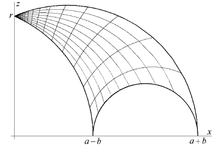
Figure 1: The admissible points in the $(x,z)$-plane.

Let $\Pi_{1}$ be the rectangle in $(s_{1},s_{2})$-plane with the vertices $s_{1}=\pm a$, $s_{2}=\pm b$. To solve system (34) express

$$\begin{array}[]{c}\displaystyle{x^{2}+z^{2}-\tau=[s_{1}+s_{2}-{\tau\over{r^{2}}}(s_{1}-s_{2})]x,}\\ \displaystyle{\Psi_{+}(x,z)=x^{2}\Lambda_{+}\Lambda_{-},\quad\Psi_{-}(x,z)=x^{2}{\rm M}_{+}{\rm M}_{-},}\end{array}$$ (36)

where

$$\begin{array}[]{l}\displaystyle{\Lambda_{\pm}(s_{1},s_{2})=s_{1}+s_{2}-{{\tau-2s\chi}\over{r^{2}}}(s_{1}-s_{2})\pm 2s,}\\ \displaystyle{{\rm M}_{\pm}(s_{1},s_{2})=s_{1}+s_{2}-{{\tau+2s\chi}\over{r^{2}}}(s_{1}-s_{2})\pm 2s.}\end{array}$$

It follows from (34), (36) that

$$\Lambda_{+}(s_{1},s_{2})\Lambda_{-}(s_{1},s_{2})\geqslant 0,\quad{\rm M}_{+}(s_{1},s_{2}){\rm M}_{-}(s_{1},s_{2})\leqslant 0.$$ (37)

Consider the parallelogram $\Pi_{2}$ bounded by the lines $\Lambda_{\pm}=0$, ${\rm M}_{\pm}=0$. The solutions of system (37) fill two half-strip regions starting at the sides of $\Pi_{2}$ belonging to the lines $\Lambda_{\pm}=0$. The example of the RPM in the $(s_{1},s_{2})$-plane, i.e., the set of solutions of inequalities (35), (37) is shown in Fig. 2.

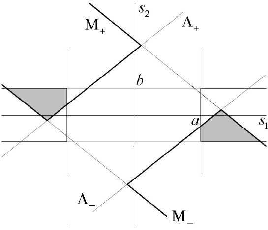
Figure 2: The example of a region of possible motions $(a=1,\;b=0.4,\;\tau=1.2,\;s=-0.6)$.

The further investigation is purely technical. The bifurcations of the RPM’s take place in one of the following cases: the vertex of one parallelogram out of $\Pi_{1},\Pi_{2}$ resides on the boundary of another; the sides of the parallelograms $\Pi_{1},\Pi_{2}$ happen to be respectively parallel (the vertices of the RPM go to the infinity); the half stripe region degenerates and becomes a half line. Finding all such cases gives the equations for $s,\tau$ pointed out in the theorem. Let $\Delta$ denote the set defined by these equations in ${\bf{R}}^{2}(s,\tau)$. Considering the connected components of ${\bf{R}}^{2}(s,\tau)\backslash\Delta$ we ignore those of them which correspond to the empty RPM’s. The rest of components (the admissible regions in the integral constants space) are shadowed in Fig. 3. The bifurcation diagram consists of those segments of $\Delta$ that are boundaries of the admissible regions excluding the parts of the axis $s=0$ since this value of $s$ is not admissible by virtue of (18). This way we obtain the inequalities needed. The theorem is proved.∎

5 On the possibility of the separation of variables

Denote

$$\xi=x^{2}+z^{2}-\tau$$

and consider the following second-order surface in the $(x,\xi,\mu)$-space

$$\mu^{2}=\tau\xi^{2}+\sigma x^{2}-\tau\sigma.$$ (38)

Due to the second equation in (33) each trajectory is represented by some curve on this surface.

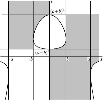
Figure 3: Region of existence of motions in the $(s,\tau)$-plane.

Obviously, the constants $\tau,\sigma$ cannot be simultaneously negative. Therefore, surface (38) has two families of rectilinear generators.

The introduced constants satisfy the following two identities

$$\sigma+2\tau(p^{2}\pm r^{2})=(\tau\pm r^{2})^{2}.$$ (39)

It is easily seen that by virtue of (32), (39) the equations $\Phi_{\pm}=0$, $\Psi_{\pm}=0$ in the $(x,\xi)$-plane define the family of lines tangent to the cross section of surface (38) by the plane $\mu=0$. Such line is then the projection of some generator of surface (38). Since each point on surface (38) belongs exactly to two generators the parameters of the latter can be chosen as local coordinates in the region in the $(x,\xi)$-plane covered by surface (38).

Not regarding any reality conditions, put formally

$$\xi=\sqrt{\sigma}{{uv+1}\over{u+v}},\quad x=\sqrt{\tau}{{u-v}\over{u+v}}.$$

After some simple transformations we get

$$\begin{array}[]{l}\displaystyle{\Phi_{+}={1\over{(u+v)^{2}}}\varphi_{1}(u)\varphi_{1}(v),\quad\Phi_{-}={1\over{(u+v)^{2}}}\varphi_{2}(u)\varphi_{2}(v),}\\ \displaystyle{\Psi_{+}={1\over{(u+v)^{2}}}\psi_{1}(u)\psi_{1}(v),\quad\Psi_{-}={1\over{(u+v)^{2}}}\psi_{2}(u)\psi_{2}(v),}\end{array}$$

where

$$\begin{array}[]{ll}\varphi_{1}(w)=\sqrt{\sigma}(1+w^{2})+2(\tau+r^{2})w,&\varphi_{2}(w)=\sqrt{\sigma}(1+w^{2})+2(\tau-r^{2})w,\\ \psi_{1}(w)=\sqrt{\sigma}(1+w^{2})+4s\chi w,&\psi_{2}(w)=\sqrt{\sigma}(1+w^{2})-4s\chi w.\end{array}$$

In the plane of the variables $u,v$ inequalities (29), (34) define the set of rectangles with the sides parallel to the coordinate axes. The fact that each connected component of any integral manifold is represented by such a rectangle (and in the case of a bifurcation by a segment or a pair of rectangles having a common side) means that in these variables the equations of motion must separate. The corresponding calculations are too long for the restricted volume of this article and will be presented in another publication. We only point out the connections with the above results.

Consider the polynomial

$$Q(w)=\varphi_{1}(w)\varphi_{2}(w)\psi_{1}(w)\psi_{2}(w)$$ (40)

and find all the cases when it has a multiple root. The resultant of $Q(w)$ and $Q^{\prime}(w)$ in $w$ is (up to the constant multiplier)

$$s^{4}\tau^{12}(\tau^{2}-2p^{2}\tau+r^{4})^{14}[2s^{2}-(p^{2}-r^{2})]^{4}[2s^{2}-(p^{2}+r^{2})]^{4}[\tau^{2}-2(p^{2}-2s^{2})\tau+r^{4}]^{2}.$$ (41)

As it was already mentioned, by virtue of equations (18) at the considered family of motions we have $s\neq 0$. The rest of cases when expression (41) vanishes lead to the equations listed in Theorem 3. Therefore, the bifurcation diagram found above is the part of the discriminant set of polynomial (40). Such phenomenon is also typical for the systems with algebraically separating variables.

References

- [1] Appelrot G.G. Non-completely symmetric heavy gyroscopes // In: Motion of a rigid body about a fixed point, Collection of papers in memory of S.V.Kovalevskaya. – Moscow-Leningrad. – 1940. – P. 61-156. (In Russian)
- [2] Bogoyavlensky O.I. Euler equations on finite-dimension Lie algebras arising in physical problems // Commun. Math. Phys. – 1984. – 95. – P. 307-315.
- [3] Kowalevski S. Sur le probleme de la rotation d’un corps solide autour d’un point fixe // Acta Mathematica. – 1889. – 2. – P. 177-232.
- [4] Reyman A.G., Semenov-Tian-Shansky M.A. Lax representation with a spectral parameter for the Kowalewski top and its generalizations // Lett. Math. Phys. – 1987. – 14, 1. – P. 55-61.
- [5] Kharlamov M.P. The critical set and the bifurcation diagram of the problem of motion of the Kowalevski top in double field // Mekh. Tverd. Tela. – 2004. – N 34. – P. 47-58. (In Russian) Engl. vers. Kharlamov M.P. Bifurcation diagrams of the Kowalevski top in two constant fields // Regular and Chaotic Dynamics. – 2005. – 10, 4. – P. 381-398.
- [6] Kharlamov M.P. One class of solutions with two invariant relations of the problem of motion of the Kowalevski top in double constant field // Mekh. Tverd. Tela. – 2002. – N 32. – P. 32-38. (In Russian) Engl. transl. http://arxiv.org/abs/0803.1028v1.
- [7] Kharlamov M.P., Savushkin A.Yu. Separation of variables and integral manifolds in one problem of motion of generalized Kowalevski top // Ukrainian Mathematical Bulletin. – 2004. – 1, 4. – P. 569-586.
- [8] Kharlamov M.P., Savushkin A.Yu., Shvedov E.G. Bifurcation set in one problem of motion of the generalized Kowalevski top // Mekh. Tverd. Tela. – 2003. – N 33. – P. 10-19. (In Russian)
- [9] Zotev D.B. Fomenko-Zieschang invariant in the Bogoyavlenskyi case // Regular and Chaotic Dynamics. – 2000. – 5, 4. – P. 437-458.