NEW PERSPECTIVES FOR HEAVY FLAVOUR PHYSICS FROM THE LATTICE

Heavy flavours represent a challenge for lattice QCD. We discuss it in very general terms. We give an idea of the significant recent progress which opens up good perspectives for high precision first principles QCD computations for flavour physics.

1 Overview

In this talk I want to convey an idea about the perspectives for precise lattice QCD computations. Some emphasis is put on the field of flavour physics, where lattice QCD seems to be needed the most in the quantitative interpretation of present and future experiments (in particular this is the reason for Sect. 4.3). I do not want to discuss the latest numbers but will focus on the principle, the challenges and the perspectives. I mainly address those in the audience who know little about the field and therefore take a bit of a bird’s-eye view of the field. So I do not hesitate to also list trivial facts (e.g. Sect. 4.2) and my personal opinion on what is relevant for the future.

2 The principle

We want to find answers for properties of QCD in the non-perturbative domain, where the usual power series expansion in the coupling constant fails completely. This is done through a
     Monte Carlo (MC) evaluation
     of the Euclidean path integral
     after a discretization of space-time on a lattice with spacing $a$ in all 3+1 dimensions.
The last of these items seems like a bad mutilation of the theory, but we emphasize that discretization is just one form of regularization, i.e. the taming of the infamous UV divergences of continuum path integrals. In fact discretization is the only known, complete regularization of the theory: complete in the sense that it defines the theory mathematically also beyond an expansion in the coupling.

In lattice QCD the Euclidean path integral is “solved” numerically. Many observables can be computed directly in Euclidean space-time, but even more cannot be computed (unless the complete dependence on time is known). Examples are scattering cross sections.

What at first sight looks like the (classical) coupling constant, $g_{0}$, and quark masses, $m_{0,i}$, have no direct physical meaning in a quantum field theory such as QCD. They are bare (actually divergent) quantities which need renormalization. In the general (non-perturbative) case, renormalization just means that the bare parameters are replaced by observable quantities. It is convenient to parametrize the theory as follows. The MC evaluation of the path integral yields dimensionless hadron masses (remember that $a$ is the lattice spacing),

$$am^{\mathrm{had}}_{h}=\mu^{\mathrm{had}}_{h}(g_{0},\{\,\mu^{\mathrm{quark}}_{i}\,\})$$ (1)

as a function of the bare, dimensionless, parameters in the Lagrangian of the theory, $g_{0},\;\mu^{\mathrm{quark}}_{i}=am^{\mathrm{quark}}_{0,i}\,,\;i={\rm u},{\rm d},\ldots$. We consider the theory with $N_{\rm f}$ quarks and require $N_{\rm f}$ ratios of hadron masses to agree with Nature. This may be read as fixing the bare dimensionless quark masses $\mu_{i}$ to the correct values at a given $g_{0}$. Taking now in addition the dimensionfull masse(s) $m_{h}$ from experiment, yields the lattice spacing

$$a={\mu^{\mathrm{had}}_{h}\over m_{h}}=a(g_{0})\,,$$ (2)

for any value of the bare coupling $g_{0}$. At this point the theory is parametrized in terms of physical observables namely $N_{\rm f}+1$ hadron masses. A new observable, e.g. the B-meson decay constant, $F_{\rm B}$, relevant for flavour physics, is now a function 

$$F_{\rm B}=F_{\rm B}(a,m_{p},m_{\pi},\ldots)\,.$$ (3)

With the typical approximation of neglecting the u–d quarkmass difference as well as the influence of the top-quark on low–energy QCD, a useful set to be chosen in eq. (3) is

$$m_{p}=938.3\,{\rm MeV}\,,\;m_{\pi}=139.6\,{\rm MeV}\,,\;m_{\rm K}=493.7\,{\rm MeV}\,,\;m_{\rm D}=1896\,{\rm MeV}\,,\;m_{\rm B}=5279\,{\rm MeV}\,.$$

We observe that this experimental input is very precise. Using it as the starting point, the running renormalized quark masses and coupling can be computed (at high momentum scale) as well as other quantities; in particular matrix elements needed for flavour physics, such as $F_{\rm B}$.

Of course the continuum limit $a\to 0$ has to be taken to arrive at the physical quantity, $F_{\rm B}(0,m_{p},m_{\pi},\ldots)$. The only assumption is that this limit exists. (In practise, it is taken by a numerical extrapolation of a few data points at different $a$.) There is a large amount of evidence, perturbative and non-perturbative and also from the investigation of critical phenomena, that given a local action (that means a discretization with exponentially localized interactions) the continuum limit does exist. The perturbative renormalization group self-consistently predicts that the continuum limit is at $g_{0}=0$: $a(0)=0$.

2.1 Some results

In recent years more and more results have appeared with rather small quoted error bars. We refer the reader to reviews by M. Della Morte and A. Jüttner at “Lattice 2007” $\!{}^{{\bf?},{\bf?}}$ and, focusing more on recent results, the one of E. Gamiz at “Lattice 2008” $\!{}^{{\bf?}}$. In Table 1 we collected a few quantities, interesting for flavour physics, for which errors around 1 % are quoted $\!{}^{{\bf?}}$.

$m_{{\rm c}}^{{\rm\overline{MS\kern-0.35002pt}\kern 0.35002pt}}(3\,{\rm GeV})$	=	$0.986(10)\,{\rm GeV}$	HPQCD $\!{}^{{\bf?}}$
$m_{{\rm b}}^{{\rm\overline{MS\kern-0.35002pt}\kern 0.35002pt}}(m_{{\rm b}})$	=	$4.20(4)\,{\rm GeV}$	HPQCD $\!{}^{{\bf?}}$
$\xi={F_{\rm B_{\rm s}}\sqrt{m_{\rm B_{\rm s}}}\over F_{\rm B}\sqrt{m_{\mathrm{B}}}}$	=	$1.211(38)(24)$	FNAL/MILC $\!{}^{{\bf?}}$
$F_{\rm B_{\rm s}}$	=	$243(11)\,{\rm MeV}$	FNAL/MILC $\!{}^{{\bf?}}$
$F_{\rm D_{\rm s}}$	=	$241(3)\,{\rm MeV}$	HPQCD $\!{}^{{\bf?}}$

Table 1: Results discussed in the review of E. Gamiz $\!{}^{{\bf?}}$.

Taken at face value, the last line in the table is in disagreement with what the CLEO experiment finds; see the talk of Philip Rubin at this conference. Should we conclude in favour of new physics $\!{}^{{\bf?}}$, or is this precocious? As a preparation for an answer to this question, we take a rough look at the machinery used in practise to obtain the results.

2.2 The machinery

At this point in time, the numbers with the smallest quoted error bars come from so-called rooted staggered fermion simulations (all those in Table 1 do). There are serious concerns about the validity of this formulation, see for example $\!{}^{{\bf?}}$. Since a local action equivalent to rooted staggered fermions is not known, the arguments justifying the rooting trick represent an involved discussion based on additional assumptions. $\!{}^{{\bf?},{\bf?}}$

Also NRQCD is used for the b-quark in the analysis which yields Table 1. As an effective field theory it contains power divergences; this means terms that diverge as $1/a^{n}$. In lattice NRQCD they are subtracted perturbatively. Uncancelled divergences of the form

$${g_{0}^{2(k+1)}\over a\;m_{b}}\sim{1\over a\,[\log(a)]^{k}m_{{\rm b}}}\;\raisebox{-0.43057pt}{ $\stackrel{{\scriptstyle\small{a\to 0}}}{{\longrightarrow}}$}\;\infty\,$$ (4)

are then left behind when one works until $k$’th order in perturbation theory. The continuum limit therefore does not exist and the estimate of the precision of extracted results is delicate. Other sophistications commonly employed include smearing, many parameter fits (in the case of staggered chiral perturbation theory) and Baysian fits.

All in all the large amount of tricks employed in the computations compromises their directness and “first principles status”. One could also say systematic errors might be underestimated. It is often emphasized that the methods are tested by a comparison to experimental numbers. In our opinion, this is appropriate for gaining a rough idea on the validity range of model calculations, but not the way to establish a controlled theory computation. Before concluding that new physics is present, it appears very desirable to perform independent computations with an independent technology. In particular we insist on

• a manifestly local discretization and

• non-perturbative subtraction of power law divergences.

Such computations are in progress. Before turning to them, let us understand why they were not carried out already a number of years ago. The basic reason is that lattice QCD is a considerable challenge.

3 The challenge

This becomes apparent by considering just the typical hadronic input eq. (3). There is a large range of scales between $m_{\pi}\approx 140\,{\rm MeV}$ over $m_{\rm D}=2\,{\rm GeV}$ to $m_{\rm B}=5\,{\rm GeV}$. In addition, the ultraviolet cutoff of $\Lambda_{\rm UV}=a^{-1}$ of the discretized theory has to be large compared to all physical energy scales if the discretised theory is to be an approximation to a continuum. Also the linear extent of space time has to be restricted to a finite value $L$ in a numerical treatment: there is an infrared cutoff $L^{-1}$. Together the following constraints have to be satisfied.

$$\Lambda_{\rm IR}\;=\;L^{-1} \ll\;m_{\pi}\,,\;\ldots\;,m_{\rm D}\,,m_{\rm B}\;\ll a^{-1}\;=\;\Lambda_{\rm UV}$$

$$\mbox{effects}\qquad\qquad\qquad{\rm O}({\rm e}^{-Lm_{\pi}}) {\rm O}((a\,m^{\mathrm{had}})^{2})$$

$$\downarrow \downarrow$$

$$L\gtrsim 4/m_{\pi}\approx 6\,{\rm fm} a\lesssim 1/(2m_{\rm D})\approx 0.05\,{\rm fm}\qquad\qquad$$

yielding $$L/a\gtrsim 120\,.$$

After the first line, we have discarded the scale of mesons or baryons with b-quarks. Thus these are not included in the already rather intimidating estimate of $L/a\gtrsim 120$. Looking at these numbers, it appears unavoidable to separate the b-quark mass scale from the others before simulating the theory. We shall return to this in Sect. 4.3.

4 Perspectives

Despite the considerable challenge that we are facing, there are good perspectives for meeting it soon. First, without being able to enter into the merited in-depth discussion, I mention that the condition $L\gtrsim 6\,{\rm fm}$ may be relaxed by choosing unphysically large pion masses combined with a subsequent extrapolation. A factor of 1.5 to 2 may be gained this way. Such extrapolations are theoretically guided by chiral perturbation theory $\!{}^{{\bf?}}$, also including lattice spacing effects $\!{}^{{\bf?},{\bf?}}$.

Figure 1: Performance of DD-HMC as a function of the inverse quark mass $\!{}^{{\bf?}}$. “Accelerated DD-HMC” refers (amongst others) to the use of deflation. Note that the cpu-time $t$ for original HMC algorithm scales with $(am_{\mathrm{sea}})^{-n}\,,\;n\geq 3$.

4.1 Algorithms

Second, it is not obvious what is the CPU-effort for a QCD simulation. Indeed, since the development of the first exact algorithm called Hybrid Monte Carlo (HMC) $\!{}^{{\bf?}}$, it has been improved considerably  by multiple time-scale integration $\!{}^{{\bf?},{\bf?}}$, the Hasenbusch trick of mass-preconditioning $\!{}^{{\bf?},{\bf?}}$, the use of the domain decomposition method in QCD $\!{}^{{\bf?},{\bf?},{\bf?}}$ and a deflation method $\!{}^{{\bf?}}$ combined with chronological inverters $\!{}^{{\bf?}}$. In parallel, parameters of the algorithms may be tuned $\!{}^{{\bf?}}$ and it has been understood that instabilities due to the breaking of chiral symmetry become irrelevant in sufficiently large volumes $\!{}^{{\bf?}}$. Also algorithms for the contributions of single flavours (not mass-degenerate within a doublet) have been developed $\!{}^{{\bf?},{\bf?}}$. It is further suggested that fluctuations at small quark masses can be tamed by clever reweighting techniques $\!{}^{{\bf?},{\bf?}}$.

Amongst all these developments, we emphasize the recent taming of the critical slowing down with the quark mass. It was achieved by M. Lüscher through a combination of deflation with others of the tricks listed above. The impressive weak dependence of the execution time on the quark mass is illustrated in Fig. 1 taken from $\!{}^{{\bf?}}$.

4.2 Machines

It is well known that the speed of computers has been increasing continuously – at an exponential rate. Yet, it is illustrative to look at an (incomplete and personal) list of the machines available over the years. Tflop numbers have to be taken with care, but the overall message on the fast growth of available computer power is clear. Because of recent investments into high performance computing, the growth has been stronger than Moore’s law.

year	machine	speed/Tflops	share for a typical
			LQCD collaboration
1984	Cyber205	0.0001	/100
1994	APE100	0.0500	/4
2001	APE1000	0.5000	/4
2005	apeNEXT	2.0000	/3
2009	PC-Cluster “Wilson”	15.0000	/1
2009	BG/P	1000.0000	/20(?)

Table 2: An incomplete list (in particular between 1984 and 1994 there were a number of other machines) of computers on which we have done QCD computations.

Figure 2: HQET strategy. The parameters in the HQET Lagrangian and fields are denoted by $\omega_{k}$. In the matching step they are directly determined from requiring $\Phi^{\rm HQET}_{i}(a,L_{1},m_{{\rm b}})=\Phi^{\rm QCD}_{i}(a=0,L_{1},m_{{\rm b}})$ (other masses are supressed). In a second step they are used to compute $\Phi^{\rm HQET}_{i}(a=0,L_{2}=2L_{1},m_{{\rm b}})$ by an extrapolation in $a_{1}$. Returning to finite $a$, allows to extract $\omega_{k}(a_{2})$ at larger lattice spacings $a_{2}$. These are sufficient for infinite volume computations. The r.h.s. shows the same procedure understood as a relation between renormalized quantities.

4.3 Strategies for the b-quark

B-meson decays and mixing are an essential part of flavour physics. We have seen above that their direct, “relativistic”, treatment is impossible, since the demand of $L/a\gtrsim 120$ would be increased by yet another factor of 2-3. Conversely we may, however, also use the large mass of the b-quark to our advantage, working in an expansion in $\Lambda_{\mathrm{QCD}}/m_{{\rm b}}$. There are kinematical limitations to this expansion: momenta of other particles also have to be small compared to the b-quark mass. This means for example that the larger part of phase space in a decay $B\to\pi l\nu$ is not accessible to HQET, the effective field theory which implements the expansion. In the analysis of the experimental data an apropriate cut has to be implemented.

The most significant difficulty in a non-perturbative use of HQET is, however, of a different origin. We already mentioned power law divergences in Sect. 2.2. These appear in the effective theory and have to be subtracted non-perturbatively, which means the parameters of the effective theory have to be determined non-perturbatively, thus avoiding terms of the form eq. (4). In contrast to QCD, new parameters appear at each order in the HQET expansion. Still, their determination follows the logic as described around eq. (1). There is only one twist to the general principle: instead of using a relatively large number of experimental inputs, which results in a loss of predictive power , one may compute quantities in lattice QCD with a relativistic b-quark and use those as input. This step is denoted by non-perturbative matching. It was realized already a while ago $\!{}^{{\bf?},{\bf?}}$ that such a strategy can be carried out by considering quantities defined in a finite volume of linear dimension around $L=0.2\ldots 0.5\,{\rm fm}={\rm O}(1/\Lambda_{\mathrm{QCD}})$ in this initial step. Some technical obstacles had to be removed $\!{}^{{\bf?},{\bf?},{\bf?},{\bf?}}$, but now the path appears paved for a precise implementation of the idea. The strategy is depicted in Fig. 2.

An impression of the achievable precision may be gained from the pioneering computation $\!{}^{{\bf?}}$, where for the first time $1/m_{\mathrm{b}}$ corrections were taken into account. We warn the reader that this was a quenched computation, where sea-quark effects are ignored. It should be used to judge on the achievable precision, not for input into phenomenology. The computation focussed on the relation between the (spin-averaged) B-meson mass and the renormalization group invariant b-quark mass, $M_{{\rm b}}$. Table 3 displays the results for $M_{{\rm b}}$ at the lowest order in $1/m_{\mathrm{b}}$. Units are the potential scale $\!{}^{{\bf?}}$ $r_{0}\approx 0.5\,{\rm fm}$. The second column of the table lists the results in the static approximation, where terms of order $\Lambda$ in $M_{{\rm b}}$ are included, while corrections of order $\Lambda^{2}/m_{{\rm b}}^{2}$ relative to the leading term are omitted. Since the computation is carried out with different matching conditions, specified by an angle $\theta_{0}$ appearing in the boundary conditions for the quarks, their spread of about 3% can be taken as an indication for the size of the corrections. At the next order in $1/m_{\mathrm{b}}$ (columns 3–5), even more different matching conditions are explored (angles $\theta_{1},\theta_{2}$). The spread of results is now reduced to a level of below 1 part in 200, much smaller than the total error of the result . We conclude that precision computations are possible in HQET.

$\theta_{0}$	$r_{0}\,M_{\rm b}^{(0)}$		$r_{0}\,M_{\rm b}=r_{0}\,(M_{\rm b}^{(0)}+M_{\rm b}^{(1a)}+M_{\rm b}^{(1b)})$
			$\theta_{1}=0$	$\theta_{1}=1/2$	$\theta_{1}=1$
			$\theta_{2}=1/2$	$\theta_{2}=1$	$\theta_{2}=0$
		Main strategy
0	17.25(20)		17.12(22)	17.12(22)	17.12(22)
		Alternative strategy
0	17.05(25)		17.25(28)	17.23(27)	17.24(27)
1/2	17.01(22)		17.23(28)	17.21(27)	17.22(28)
1	16.78(28)		17.17(32)	17.14(30)	17.15(30)
	3 %	$0.6\%\ll$ total error
	$={\rm O}(\Lambda^{2}/m_{{\rm b}}^{2})$	$={\rm O}(\Lambda^{3}/m_{{\rm b}}^{3})$

Table 3: Renormalization group invariant b-quark mass. $\Lambda\equiv\Lambda_{\mathrm{QCD}}$.

As a preparation for a discussion of a second method for implementing the scale separation, let us turn to the right part of Fig. 2. There the procedure is interpreted as a relation

$$\Phi^{\rm QCD}(a_{0},L_{1},m_{{\rm b}})=\Phi^{\rm HQET}(a_{1},L_{1},m_{{\rm b}})\;\to\Phi^{\rm HQET}(a_{1},L_{2},m_{{\rm b}})=\Phi^{\rm HQET}(a_{2},L_{2},m_{{\rm b}})\qquad$$

$$\qquad\qquad\qquad\qquad\;\to\mbox{large volume physics}$$

The fact that only observables appear in this chain, with the parameters in the Lagrangian of the theory eliminated, makes clear that the continuum limits $a_{i}\to 0$ can be taken in each step. In practise, $a_{0}$ down to $0.01\,{\rm fm}$ is used while $a_{2}$ ranges between $0.05\,{\rm fm}$ and $0.1\,{\rm fm}$.

The second method starts from the same idea and the same (or similar) quantities in $L=L_{1}$. But then it remains in relativistic QCD, computing

$$\sigma_{i}(L_{1})=\lim_{m_{\mathrm{h}}\to m_{{\rm b}}}\lim_{a_{1}\to 0}{\Phi^{\rm QCD}_{i}(a_{1},L_{2},m_{\mathrm{h}})\over\Phi^{\rm QCD}_{i}(a_{1},L_{1},m_{\mathrm{h}})}\,,$$ (5)

for each desired observable $\Phi^{\rm QCD}_{i}$. Similarly one connects to the large volume in the last step $\!{}^{{\bf?},{\bf?}}$. The advantage is that there are no truncation errors of order $1/m_{\mathrm{b}}^{2}$. On the downside, lattice spacings $a_{1},a_{2}$ have to be considerably smaller and/or the masses $m_{\mathrm{h}}$ in the numerical extrapolation $m_{\mathrm{h}}\to m_{{\rm b}}$ have to be significantly smaller than the physical one. However, the combination $L_{i}m_{\mathrm{h}}$ is always large compared to one and therefore a smooth extrapolation of the functions $\sigma_{i}$ in $1/(L_{i}m_{\mathrm{h}})$ is expected and found numerically. A most promising approach is to combine the advantages of the two methods $\!{}^{{\bf?}}$. In fact, let us compare

$$\kern 1.0pt\overline{\kern-1.0ptm\kern-1.0pt}\kern 1.0pt^{{\rm\overline{MS\kern-0.35002pt}\kern 0.35002pt}}_{{\rm b}}(\kern 1.0pt\overline{\kern-1.0ptm\kern-1.0pt}\kern 1.0pt_{\rm b}) = 4.347(48){\rm GeV}\qquad\mbox{HQET~{}\immediate{$\!{}^{{\bf?}}$}}$$

quenched!

$$\kern 1.0pt\overline{\kern-1.0ptm\kern-1.0pt}\kern 1.0pt^{{\rm\overline{MS\kern-0.35002pt}\kern 0.35002pt}}_{{\rm b}}(\kern 1.0pt\overline{\kern-1.0ptm\kern-1.0pt}\kern 1.0pt_{\rm b}) = 4.421(67){\rm GeV}\qquad\mbox{combination~{}\immediate{$\!{}^{{\bf?}}$}}$$

The comparison is meaningful because the experimental inputs (which matter in the quenched approximation) have been chosen the same. Let us finally note that the dominating uncertainty here is the one in the renormalization factor for the quark mass in the relativistic theory $\!{}^{{\bf?},{\bf?}}$; this can be improved.

We emphasize that dynamical fermions are absolutely needed for a comparison to phenomenology. Presently, these strategies are being applied to $N_{\rm f}=2$ QCD (just up and down sea). An intermediate result $\!{}^{{\bf?}}$ shown in Fig. 3 demonstrates the precision of the most difficult continuum extrapolations.

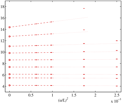
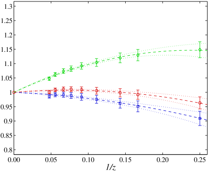
Figure 3: Example of a continuum limit $\lim_{a_{0}\to 0}\Phi^{\rm QCD}(a_{0},L_{1},m_{{\rm b}})$ for a whole range of $m_{{\rm b}}$ (left) and the resulting mass dependence on the right $\!{}^{{\bf?}}$. The variable $z$ is the dimensionless RGI quark mass $z=M_{{\rm b}}L$. Curves are a low order HQET-representation. For details see the reference.

4.4 The CLS strategy

While the numerical effort for the physically small lattices (see Fig. 2) is quite modest for today’s computers, the theoretical setup is to be chosen with care. In particular the Schrödinger functional is used $\!{}^{{\bf?},{\bf?}}$ where Dirichlet boundary conditions in time play a prominent rôle. This again calls for a simple, very local action.

Such an action, the ${\rm O}(a)$-improved Wilson action $\!{}^{{\bf?},{\bf?},{\bf?}}$ is then also needed in the large volume part. The strategy of the CLS effort $\!{}^{{\bf?}}$ is to use it and through its simplicity be able to profit from developments in algorithms $\!{}^{{\bf?}}$. This helps to diminish systematic and statistical errors by working at small lattice spacings and on physically large volumes. Furthermore perturbative errors and in particular divergences (such as eq. (4)) are removed by non-perturbative calculations in the Schrödinger functional .

The present goal are simulations with $N_{\rm f}=2$ dynamical quarks, lattice spacings $a=0.08,0.06,0.04\,{\rm fm}$, sizes $L=2\,{\rm fm}$ to $4\,{\rm fm}$ and pion masses down to $m_{\pi}=200\,{\rm MeV}$. Concerning heavy flavours both the B-physics programme emphasized above and charm physics $\!{}^{{\bf?}}$ are being investigated. We note that a considerable problem remaining will have to be solved along the way: the slow evolution of topological modes $\!{}^{{\bf?}}$ in standard MC algorithms.

5 Conclusions

It is now widely recognized that lattice QCD is an important tool for computing phenomenologically relevant quantities. I have often heard complaints that progress is slow, but one has to recognize that the rich dynamics and the many relevant scales in QCD represent quite a challenge (Sect. 3). Despite this we appear to approach the era of controlled precision predictions in time for an accurate analysis of present and future flavour physics data and models. In particular present worries about the use of the rooting trick and uncancelled power divergences can become history.

References

References

- [1] M. Della Morte, PoS LAT2007 (2007) 008, 0711.3160.
- [2] A. Juttner, PoS LAT2007 (2007) 014, 0711.1239.
- [3] E. Gamiz, (2008), 0811.4146.
- [4] HPQCD, I. Allison et al., Phys. Rev. D78 (2008) 054513, 0805.2999.
- [5] C. Bernard et al., PoS LATTICE2008 (2008) 278, 0904.1895.
- [6] HPQCD, E. Follana et al., Phys. Rev. Lett. 100 (2008) 062002, 0706.1726.
- [7] B.A. Dobrescu and A.S. Kronfeld, Phys. Rev. Lett. 100 (2008) 241802, 0803.0512.
- [8] M. Creutz, (2008), 0810.4526.
- [9] S.R. Sharpe, PoS LAT2006 (2006) 022, hep-lat/0610094.
- [10] M. Golterman, (2008), 0812.3110.
- [11] J. Gasser and H. Leutwyler, Ann. Phys. 158 (1984) 142.
- [12] S.R. Sharpe and J. Singleton, Robert L., Phys. Rev. D58 (1998) 074501, hep-lat/9804028.
- [13] O. Bar, G. Rupak and N. Shoresh, Phys. Rev. D70 (2004) 034508, hep-lat/0306021.
- [14] M. Lüscher, JHEP 12 (2007) 011, 0710.5417.
- [15] S. Duane et al., Phys. Lett. B195 (1987) 216.
- [16] A.D. Kennedy, In Perspectives in Lattice QCD, World Scientific 2008 (2006), hep-lat/0607038.
- [17] J.C. Sexton and D.H. Weingarten, Nucl. Phys. B380 (1992) 665.
- [18] C. Urbach et al., Comput. Phys. Commun. 174 (2006) 87, hep-lat/0506011.
- [19] M. Hasenbusch, Phys. Lett. B519 (2001) 177, hep-lat/0107019.
- [20] M. Hasenbusch and K. Jansen, Nucl. Phys. B659 (2003) 299, hep-lat/0211042.
- [21] M. Lüscher, JHEP 05 (2003) 052, hep-lat/0304007.
- [22] M. Lüscher, Comput. Phys. Commun. 156 (2004) 209, hep-lat/0310048.
- [23] M. Lüscher, Comput. Phys. Commun. 165 (2005) 199, hep-lat/0409106.
- [24] R.C. Brower et al., Nucl. Phys. B484 (1997) 353, hep-lat/9509012.
- [25] ALPHA, H.B. Meyer et al., Comput. Phys. Commun. 176 (2007) 91, hep-lat/0606004.
- [26] L. Del Debbio et al., JHEP 02 (2006) 011, hep-lat/0512021.
- [27] R. Frezzotti and K. Jansen, Nucl. Phys. B555 (1999) 395, hep-lat/9808011.
- [28] M.A. Clark and A.D. Kennedy, (2006), hep-lat/0608015.
- [29] A. Hasenfratz, R. Hoffmann and S. Schaefer, Phys. Rev. D78 (2008) 014515, 0805.2369.
- [30] M. Luscher and F. Palombi, (2008), 0810.0946.
- [31] ALPHA, J. Heitger and R. Sommer, Nucl. Phys. Proc. Suppl. 106 (2002) 358, hep-lat/0110016.
- [32] ALPHA, J. Heitger and R. Sommer, JHEP 02 (2004) 022, hep-lat/0310035.
- [33] ALPHA, M. Della Morte et al., (2003), hep-lat/0307021.
- [34] M. Della Morte, A. Shindler and R. Sommer, JHEP 08 (2005) 051, hep-lat/0506008.
- [35] ALPHA, J. Heitger et al., JHEP 11 (2004) 048, hep-ph/0407227.
- [36] B. Blossier et al., JHEP 04 (2009) 094, 0902.1265.
- [37] R. Sommer, Nucl. Phys. B411 (1994) 839, hep-lat/9310022.
- [38] G.M. de Divitiis et al., Nucl. Phys. B672 (2003) 372, hep-lat/0307005.
- [39] G.M. de Divitiis et al., Nucl. Phys. B675 (2003) 309, hep-lat/0305018.
- [40] D. Guazzini, R. Sommer and N. Tantalo, JHEP 01 (2008) 076, 0710.2229.
- [41] ALPHA, M. Della Morte et al., Nucl. Phys. B713 (2005) 378, hep-lat/0411025.
- [42] ALPHA, M. Della Morte et al., Nucl. Phys. B729 (2005) 117, hep-lat/0507035.
- [43] M. Della Morte et al., PoS LATTICE2008 (2008) 226, 0810.3166.
- [44] M. Lüscher et al., Nucl. Phys. B384 (1992) 168, hep-lat/9207009.
- [45] S. Sint, Nucl. Phys. B421 (1994) 135, hep-lat/9312079.
- [46] B. Sheikholeslami and R. Wohlert, Nucl. Phys. B259 (1985) 572.
- [47] M. Lüscher et al., Nucl. Phys. B478 (1996) 365, hep-lat/9605038.
- [48] ALPHA, K. Jansen and R. Sommer, Nucl. Phys. B530 (1998) 185, hep-lat/9803017.
- [49] https://twiki.cern.ch/twiki/bin/view/CLS/WebHome .
- [50] G. von Hippel et al., PoS LATTICE2008 (2008) 227, 0810.0214.
- [51] L. Del Debbio, H. Panagopoulos and E. Vicari, JHEP 08 (2002) 044, hep-th/0204125.