On the consistent separation of scale and variance for Gaussian random fields

Abstract

We present fixed domain asymptotic results that establish consistent estimates of the variance and scale parameters for a Gaussian random field with a geometric anisotropic Matérn autocovariance in dimension $d>4$. When $d<4$ this is impossible due to the mutual absolute continuity of Matérn Gaussian random fields with different scale and variance (see Zhang [33]). Informally, when $d>4$, we show that one can estimate the coefficient on the principle irregular term accurately enough to get a consistent estimate of the coefficient on the second irregular term. These two coefficients can then be used to separate the scale and variance. We extend our results to the general problem of estimating a variance and geometric anisotropy for more general autocovariance functions. Our results illustrate the interaction between the accuracy of estimation, the smoothness of the random field, the dimension of the observation space, and the number of increments used for estimation. As a corollary, our results establish the orthogonality of Matérn Gaussian random fields with different parameters when $d>4$. The case $d=4$ is still open.

1 Introduction

A common situation in spatial statistics is when one has observations on a single realization of a random field $Y$ at a large number of spatial points $\bm{t}_{1},\bm{t}_{2},\ldots$ within some bounded region $\Omega\subset\mathbb{R}^{d}$. One is then is faced with the problem of predicting some quantity that depends on $Y$ at unobserved points in $\Omega$. For example, one may want to predict $\int_{\Omega}Y(\bm{t})d\bm{t}$ or the derivative $Y^{\prime}(\bm{t}_{0})$ where $\bm{t}_{0}$ is an unobserved point in $\Omega$. A common technique is to first estimate the covariance structure of $Y$, then predict using the estimated covariance. Typically, fully nonparametric estimation of the covariance is difficult since the observations are from one realization of the random field. In this case, it is common to consider a class of covariance structures indexed by a finite number of parameters which are then estimated from the observations (see [12] or [9] for an introduction to spatial statistical techniques).

Two common parameters found in many covariance models are an overall scale $\alpha$ and an overall variance $\sigma^{2}$. The simplest example of this model stipulates that the random field $Y$ is a scale and amplitude chance by an unknown $\alpha$ and $\sigma$ of a known random field $Z$. In particular, for a spatial domain $\Omega\subset\mathbb{R}^{d}$, $Y$ is modeled as

$$\{Y(\bm{t})\colon\bm{t}\in\Omega\}\overset{\mathcal{D}}{=}\{\sigma Z(\alpha\bm{t})\colon\bm{t}\in\Omega\}$$ (1)

where $\overset{\mathcal{D}}{=}$ denotes equality of the finite dimensional distributions. In this case, $\sigma$ is an overall amplitude (in units of $Y$) and $\alpha$ is an overall spatial scale (in units of $\bm{t}$). For a nice discussion of the roll of $\alpha$ and $\sigma$ in the Matérn autocovariance see Section 6.5 in [28].

A fundamental question is whether or not $\alpha$ and $\sigma$ are consistently estimable when the number of the observations in $\Omega$ grows to infinity. Indeed, the answer is no in general. This is immediate from the existence of self similar random fields that satisfy $\{Z(\alpha\bm{t})\colon\bm{t}\in\Omega\}\overset{\mathcal{D}}{=}\{\alpha^{\nu}Z(\bm{t})\colon\bm{t}\in\Omega\}$ for any $\alpha>0$ where $\nu$ is a fixed constant. For these self-similar processes, any two pairs $(\sigma_{1},\alpha_{1})$ and $(\sigma_{2},\alpha_{2})$ that satisfy $\sigma_{1}^{2}\alpha_{1}^{2\nu}=\sigma_{2}^{2}\alpha_{2}^{2\nu}$ give the same model in (1). This problem can also be present when $Z$ is not self similar. For example, suppose $Z$ is an isotropic Ornstein-Uhlenbeck process in dimension $d\leq 3$ (see Figure 1). In this case, if $\sigma_{1}^{2}\alpha_{1}=\sigma_{2}^{2}\alpha_{2}$ (i.e. $\nu=1/2$) the two models for $Y$ yield mutually absolutely continuous measures (when $d=1$ see [19], [32], when $d=2,3$ see [33], [28]) and therefore are impossible to discern with probability one when observing one realization of $Y$. We shall see, however, that in some cases it is possible to consistently estimate $\alpha$ and $\sigma$. Moreover, it will depend on dimension: typically the larger the dimension the more information there is to separate $\sigma$ from $\alpha$. Before we continue, we mention the work of Stein (see [25],[26]) which establishes that even if two models are mutually absolutely continuous, using the wrong model to make predictions may still yield asymptotically optimal estimates. In fact, this phenomenon can also occur for orthogonal measures when restricting to predictors that are linear combinations of the observations (see [27]).

To understand the condition $\sigma_{1}^{2}\alpha_{1}^{2\nu}=\sigma_{2}^{2}\alpha_{2}^{2\nu}$ one can look at what is called the principle irregular term of the autocovariance function (see [28]). Suppose, for exposition, that there exist constants $\delta_{2}>\delta_{1}>0$ such that the covariance structure of $Z$ satisfies

$$\text{cov}(Z(\bm{t}+\bm{h}),Z(\bm{t}))\approx c_{1}|\bm{h}|^{\delta_{1}}+c_{2}|\bm{h}|^{\delta_{2}}+p(|\bm{h}|),\quad\text{as $|\bm{h}|\rightarrow 0$}$$ (2)

where $p$ is an even polynomial and both $\delta_{1},\delta_{2}$ are not even integers. This model is not as restrictive as it seems and includes the Ornstein-Uhlenbeck process, the exponential autocovariance function $e^{-|\bm{s}-\bm{t}|^{\delta_{1}}}$ and the Matérn autocovariance function (see below). The term $c_{1}|\bm{h}|^{\delta_{1}}$ is often referred to as the principle irregular term and is instrumental in determining the smoothness of $Z$. The second term, $c_{2}|\bm{h}|^{\delta_{2}}$, is less influential but can have an observable effect depending on dimension and the magnitude of $\delta_{2}-\delta_{1}$. Now, if we model $Y$ by (1) and (2) we get

$$\text{cov}(Y(\bm{t}+\bm{h}),Y(\bm{t}))\approx c_{1}\sigma^{2}\alpha^{\delta_{1}}|\bm{h}|^{\delta_{1}}+c_{2}\sigma^{2}\alpha^{\delta_{2}}|\bm{h}|^{\delta_{2}}+\tilde{p}(|\bm{h}|),\quad\text{as $|\bm{h}|\rightarrow 0$.}$$ (3)

Therefore for two pairs of parameters $(\sigma_{1},\alpha_{1})$ and $(\sigma_{2},\alpha_{2})$, the condition $\sigma_{1}^{2}\alpha_{1}^{\delta_{1}}=\sigma_{2}^{2}\alpha_{2}^{\delta_{1}}$ ensures that the covariance models for $Y$ have the same principle irregular term. This explains the importance of the quantity $\sigma^{2}\alpha^{\delta_{1}}$. In addition, if one can estimate both coefficients $c_{1}\sigma^{2}\alpha^{\delta_{1}}$ and $c_{2}\sigma^{2}\alpha^{\delta_{2}}$ then it is possible to get separate estimates of $\sigma$ and $\alpha$. In what follows we develop consistent estimators of these two coefficients which allow consistent estimation of $\sigma$ and $\alpha$.

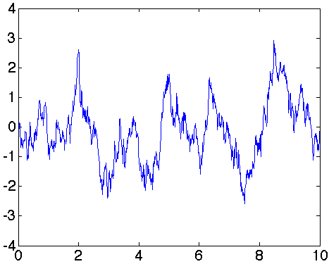
(a) $Z(2t)$

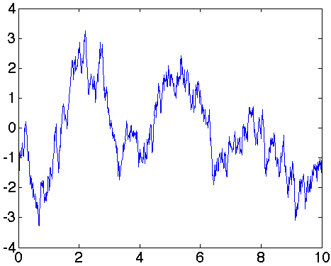
(b) $\sqrt{2}Z(t)$

Figure 1: Independent simulations of $Z(2t)$ and $\sqrt{2}Z(t)$, observed on a dense grid in $[0,10]$, where $Z$ is the Ornstein-Uhlenbeck process with covariance structure $\text{cov}(Z(s),Z(t))=e^{-|s-t|}$. In $1$, $2$ and $3$ dimensions these two processes (isotropically extended) are mutually absolutely continuous and therefore cannot be consistently distinguished under fixed domain asymptotics. Our results establish that when the dimension is greater than 4 one can distinguish the two with probability one under fixed domain asymptotics.

The majority of this paper focuses on the case when $Z$ is a mean zero, isotropic Gaussian random field which has a Matérn autocovariance. The reasons are twofold. First, the Matérn autocovariance has been used extensively in spatial statistics so that results on the Matérn autocovariance are of intrinsic interest alone. The second reason is that once one establishes the results for the Matérn it is relatively easy to see how to extend to other covariance functions. In Section 3, we give two examples that illustrate these extensions. Our Matérn assumption stipulates the existence of a known $\nu>0$ such that

$$\text{cov}(Z(\bm{s}),Z(\bm{t}))=\frac{|\bm{s}-\bm{t}|^{\nu}\mathcal{K}_{\nu}(|\bm{s}-\bm{t}|)}{2^{\nu-1}\Gamma(\nu)}$$ (4)

for all $\bm{s},\bm{t}\in\Omega\subset\mathbb{R}^{d}$ where $|\cdot|$ denotes Euclidean distance and $\mathcal{K}_{\mu}$ is the modified Bessel function of the second kind of order $\nu>0$ (see [1]). The parameter $\nu$ controls the mean square smoothness of the process: larger $\nu$ corresponds to smoother $Z$. The flexibility provided by the smoothness parameter $\nu$ along with the fact that it is positive definite in any dimension leads to its widespread use in spatial statistics.

In what follows we extend the basic model (1) to the case when there is an unknown invertible matrix $M$ with determinant 1 (this class of matrices we denote by $SL(d,\mathbb{R})$) so that

$$\{Y(\bm{t})\colon\bm{t}\in\Omega\}\overset{\mathcal{D}}{=}\{\sigma Z(\alpha M\bm{t})\colon\bm{t}\in\Omega\}.$$ (5)

The matrix $M$ is called a geometric anisotropy and is used to model a directional sheer of $Z$. The assumption that $\det M=1$ removes identifiability problems with the overall scale parameter $\alpha$. In Section 2, we construct estimates of $\sigma^{2}\alpha^{2\nu}$, $M$ and $\alpha$. We show that the estimates of $\sigma^{2}\alpha^{2\nu}$ and $M$ are strongly consistent in any dimension and the estimate of $\alpha$ is strongly consistent when $d>4$.

There is a fair amount of literature on estimating $\sigma^{2}\alpha^{2\nu}$ for the Matérn autocovariance. In 1991, Ying [32] established strong consistency and the asymptotic distribution of the maximum likelihood estimate of $\sigma^{2}\alpha^{2\nu}$ for the Ornstein-Uhlenbeck process when $d=1$ (which has a Matérn autocovariance for $\nu=1/2$). In 2004, Zhang [33] established that the maximum likelihood estimate of $\sigma^{2}\alpha^{2\nu}$ (obtained by fixing $\alpha$ and $\nu$) is strongly consistent when $d\leq 3$. In related work, Loh [23] shows that maximum likelihood estimates of scale and variance parameters in a non-isotropic multiplicative Matérn model are consistent when $\nu=3/2$ (similar results for the Gaussian autocovariance model can be found in [24]). In Section 6.7 of [28], Stein derives asymptotic properties of the maximum likelihood estimates of $\alpha$, $\sigma$ and $\nu$ for a periodic version of the Matérn random field. For this periodic random field all the parameters are consistently estimable when $d\geq 4$. Our results confirm these findings for $\alpha$ and $\sigma$ with the non-periodic Matérn when $d>4$. The case $d=4$ is still open.

Recent work by Kaufman et al.​ [8] and Du et al.​ [13] studies maximum likelihood estimates of $\sigma^{2}\alpha^{2\nu}$ using a tapered Matérn autocovariance when $d\leq 3$. The advantage gained by tapering is a reduction of the computational load for computing the likelihood and for computing kriging estimates. We will see that our estimates of the same quantity, $\sigma^{2}\alpha^{2\nu}$, yield strongly consistent estimates in any dimension which are “root n” consistent and are easily computed with no maximization required. However, our estimates depend on the grid format of the observations whereas the maximum likelihood estimates are not confined to such restrictions. We also expect some loss of efficiency in our estimates as compared to the MLE. We hope that there is potential to combine the two estimation methods using a one-Newton-step tapered likelihood adjustment to the increment based estimate. Since our results can be easily extended, by a Lindeberg-Feller argument, to obtain the asymptotic normality of $\widehat{\sigma^{2}\alpha^{2\nu}}$ when $d\leq 3$, we believe this has the potential to mitigate any loss of efficiency and reduce the computational load for the maximum likelihood estimate.

Finally we mention the long tradition of using squared increments to estimate properties of random fields, beginning with the quadratic variation theorem of Lévy in 1940 ([22]). For example, increments have been used in [20] and [6] for identification of a local fractional index and in [11] to identify the singularity function of a fractional process. In [4] they are used to estimate a deformation of an isotropic random field. For more results on the convergence of quadratic variations see, [5], [15], [14], [21], [7], [30],[2], [6], [16], [10], [20].

2 The geometric anisotropic Matérn class

In this section we construct estimates of $\sigma^{2}\alpha^{2\nu}$, $M$ and $\alpha$ using increments of $Y$ observed on a dense grid within $\Omega$. Using fixed domain asymptotics, we establish consistency of our estimates under assumptions (4) and (5) and provide bounds on the rate of variance decay as it depends on the number of increments used, the dimension of $\Omega$ and the smoothness of $Y$ measured by $\nu$. These results will hold in any dimension. However, when the dimension is large enough ($d>4$), the second term in (3) is influential enough so that $\alpha$ can be estimated consistently.

If the observation region $\Omega$ is an open subset of $\mathbb{R}^{d}$ and the random field $Y$ is modeled by (4) and (5), then $Y$ is said to be a $d$-dimensional geometric anisotropic Matérn random field with parameters $(\sigma,\alpha,\nu,M)$. In this case, the covariance structure of $Y$ is $\text{cov}(Y(\bm{s}),Y(\bm{t}))=K(|M\bm{s}-M\bm{t}|)$, where $K$ is defined as

$$K(t)\triangleq\frac{\sigma^{2}(\alpha t)^{\nu}}{\Gamma(\nu)2^{\nu-1}}\mathcal{K}_{\nu}(\alpha t)$$ (6)

for $t>0$ and $K(0)\triangleq\lim_{t\downarrow 0}K(t)=\sigma^{2}$. The function $\mathcal{K}_{\nu}$ is the modified Bessel function of the second kind of order $\nu>0$. Since $|M\bm{s}-M\bm{t}|=|OM\bm{s}-OM\bm{t}|$ for any orthogonal matrix $O$, one can only identify $M$ up to left multiplication by an orthogonal matrix. To remove this identifiability problem we suppose that $M\in SL(d,\mathbb{R})/SO(d,\mathbb{R})$ where $SO(n,\mathbb{R})$ denotes the orthogonal matrices in $SL(d,\mathbb{R})$. In the theorems below, we write $M_{1}=_{SL/SO}M_{2}$ to mean that there exists a $O\in SO(n,\mathbb{R})$ such that $M_{1}=OM_{2}$, and similarly for $M_{1}\neq_{SL/SO}M_{2}$. Operationally, however, we estimate a representer of the cosets in $SL(d,\mathbb{R})/SO(d,\mathbb{R})$ given by the upper triangular matrices which have positive diagonal elements and determinant 1 (that this is a representer follows from the QR factorization, see [18]).

As discussed in the introduction, the principle irregular term is important in determining the sample path properties of the random field $Y$. The principle irregular term for the Matérn covariance function is

$$G_{\nu}(t)\triangleq\begin{cases}\rule[-10.00002pt]{0.0pt}{25.00003pt}\dfrac{(-1)^{\nu+1}}{2^{2\nu-1}\Gamma(\nu)\Gamma(\nu+1)}t^{2\nu}\log t,&\text{if $\nu\in\mathbb{Z}$;}\\ \rule[-10.00002pt]{0.0pt}{25.00003pt}\dfrac{-\pi}{2^{2\nu}\sin(\nu\pi)\Gamma(\nu)\Gamma(\nu+1)}t^{2\nu},&\text{otherwise.}\end{cases}$$

where $G_{\nu}(0)$ is defined to be $0$. Moreover,

$$\text{cov}(Y(\bm{t}+\bm{h}),Y(\bm{t}))=\sigma^{2}G_{\nu}(|\alpha M\bm{h}|) -\nu\sigma^{2}G_{\nu+1}(|\alpha M\bm{h}|)+\epsilon(|\alpha M\bm{h}|)$$ (7)

where $\epsilon(h)=\sigma^{2}p(|h|)+o(G_{\nu+1}(|h|))$ as $|h|\rightarrow 0$ and $p$ is an even polynomial. Notice that when $M$ is the identity matrix and $\nu\notin\mathbb{Z}$, this gives the expansion (3) so that $\sigma^{2}G_{\nu}(|\alpha\bm{h}|)$ is the first principle irregular term and $-\nu\sigma^{2}G_{\nu+1}(|\alpha\bm{h}|)$ is the second term.

2.1 Estimating $\sigma^{2}\alpha^{2\nu}$ and $M$ in any dimension

Let $\Omega$ be a bounded, open subset of $\mathbb{R}^{d}$ and let $\Omega_{n}\triangleq\Omega\cap\{\mathbb{Z}^{d}/n\}$. The idea is that we will be observing $Y$ on a region, just a bit larger than $\Omega_{n}$, so that we can form the $m^{\text{th}}$ order increments of $Y$ on $\Omega_{n}$. These will then be used to estimate $M$ and $\sigma^{2}\alpha^{2\nu}$ in any dimension and additionally $\alpha$, in dimension $d>4$.

For a fixed nonzero vector $\bm{h}\in\mathbb{R}^{d}$ define the increment in the direction $\bm{h}$ by $\Delta_{\bm{h}}Y(\bm{t})\triangleq Y(\bm{t}+\bm{h})-Y(\bm{t})$ and the $m^{\text{th}}$ iterated directional increment $\Delta^{m}_{\bm{h}}Y(\bm{t})\triangleq\Delta_{\bm{h}}\Delta^{m-1}_{\bm{h}}Y(\bm{t})$. The following lemma establishes the relationship between the variance of these increments and the terms in (7) when the number of increments is sufficiently large.

Lemma 1.

Let $Y$ be a mean zero, geometric anisotropic $d$-dimensional Matérn Gaussian random field with parameters $(\sigma,\alpha,\nu,M)$. If $m$ is a positive integer such that $m>\nu+1$ and $\bm{h}\in\mathbb{R}^{d}$ is a non-zero vector, then

$$\mathsf{E}(\Delta_{\bm{h}/n}^{m}Y(\bm{t}))^{2}=\frac{a_{\nu}^{m}}{n^{2\nu}}+\frac{b_{\nu}^{m}}{n^{2\nu+2}}+o(n^{-2\nu-2})$$ (8)

as $n\rightarrow\infty$ where

$$a_{\nu}^{m} \triangleq\sigma^{2}\alpha^{2\nu}|M\bm{h}|^{2\nu}\sum_{i,j=0}^{m}(-1)^{i+j}{m\choose i}{m\choose j}G_{\nu}(|i-j|)$$ (9)

$$b_{\nu}^{m} \triangleq\sigma^{2}\alpha^{2\nu+2}|M\bm{h}|^{2\nu+2}\sum_{i,j=0}^{m}(-1)^{i+j}{m\choose i}{m\choose j}(-\nu)G_{\nu+1}(|i-j|).$$ (10)

Now we are in a position to estimate the coefficient $a_{\nu}^{m}$. Let $\#\Omega_{n}$ denote the cardinality of the finite set $\Omega_{n}\triangleq\Omega\cap\{\mathbb{Z}^{d}/n\}$ and define

$$Q^{m}_{n}\triangleq\frac{1}{\#\Omega_{n}}\sum_{\bm{j}\in\Omega_{n}}n^{2\nu}(\Delta_{\bm{h}/n}^{m}Y(\bm{j}))^{2}$$ (11)

Notice that by equation (8), $\mathsf{E}Q_{n}^{m}\rightarrow a_{\nu}^{m}$ as $n\rightarrow\infty$. In addition, since $Q_{n}^{m}$ is itself an average, one might hope that $Q_{n}^{m}$ converges to $a_{\nu}^{m}$. The following theorem shows that, indeed, this is the case. In addition, the theorem quantifies the decay of the variance of $Q_{n}^{m}$ as a function of the number of increments, the smoothness of the random field $Y$ and the dimension of the domain. The heuristic is that when the number of increments $m$ is large enough, there is sufficient decorrelation of the summands of $Q_{n}^{m}$ to guarantee convergence as $n\rightarrow\infty$. Generally, more increments leads to more spatial decorrelation and hence a reduction in variance. However, this only holds up to a point, after which taking more increments no longer effects the rate of variance decay. Finally, the higher the dimension, the more increments one needs to take to get the best rate.

Theorem 1.

Let $Y$ be a mean zero, geometric anisotropic $d$-dimensional Matérn Gaussian random field with parameters $(\sigma,\alpha,\nu,M)$ and let $\Omega$ be a bounded, open subset of $\mathbb{R}^{d}$. If $m>\nu$ then

$$Q_{n}^{m}\rightarrow a_{\nu}^{m},\quad w.p.1$$ (12)

as $n\rightarrow\infty$. Moreover, there exists a constant $c>0$ such that

$$\text{var}\,Q_{n}^{m}\leq\begin{cases}c\,n^{4(\nu-m)},&\text{if $4(\nu-m)>-d$;}\\ c\,n^{-d}\log n,&\text{if $4(\nu-m)=-d$;}\\ c\,n^{-d},&\text{if $4(\nu-m)<-d$}\end{cases}$$

for all sufficiently large $n$.

The above theorem establishes that $Q_{n}^{m}$ consistently estimates $a_{\nu}^{m}$ (which depends on $\bm{h}$). Now we show how these estimates can be used to recover $M$ and $\sigma^{2}\alpha^{2\nu}$. As was mentioned above, we suppose $M$ is upper triangular with determinant one and positive diagonal elements. After renormalizing by known constants, the values of $a_{\nu}^{m}$ allow us to consistently estimate $|\tilde{M}\bm{h}|^{2}$ where $\tilde{M}\triangleq\sigma^{1/\nu}\alpha M$ for finitely many directions $\bm{h}$. We show by induction that these values are sufficient to recover each column of $\tilde{M}$. Once this is established, the requirement $\det M=1$ gives $M=(\det\tilde{M})^{-1/d}\tilde{M}$ and $\sigma^{2}\alpha^{2\nu}=(\det\tilde{M})^{2\nu/d}$.

Let $\tilde{M}_{i,j}$ denote the $i,j^{\text{th}}$ element of $\tilde{M}$ and let $\tilde{M}_{:,i}$ denote the $i^{\text{th}}$ column of $\tilde{M}$. Also let $\tilde{M}_{1:k,1:k}$ be the submatrix with elements $\tilde{M}_{i,j}$ for $i,j=1,\ldots,k$. For the first column of $\tilde{M}$, notice that $|\tilde{M}e_{1}|=\tilde{M}_{1,1}$ where $e_{1},\ldots,e_{d}$ denote the standard basis of $\mathbb{R}^{d}$. This follows since $\tilde{M}$ is upper triangular with positive diagonal. For the inductive step suppose the first $k$ columns $\tilde{M}_{:,1}\ldots,\tilde{M}_{:,k}$ are known. Taking $\bm{h}=e_{k+1}$ and $\bm{h}=e_{k+1}-e_{i}$ allows us to recover $|\tilde{M}_{:,k+1}|^{2}$ and $|\tilde{M}_{:,k+1}-\tilde{M}_{:,i}|^{2}$ for $i=1,\ldots,k$. By adding and subtracting appropriate terms we can then recover: $\bigl{\langle}\tilde{M}_{:,k+1},\tilde{M}_{:,i}\bigr{\rangle}$, for all $i=1,\ldots,k+1$. Therefore $\tilde{M}_{:,k+1}=\Bigl{(}v,\sqrt{|\tilde{M}_{:,k+1}|^{2}-|v|^{2}},0,\ldots,0\Bigr{)}^{T}$ where $v\triangleq\tilde{M}_{1:k,1:k}^{-1}\bigl{(}\bigl{\langle}\tilde{M}_{:,k+1},\tilde{M}_{:,i}\bigr{\rangle}\bigr{)}_{i=1}^{k}$. This establishes the inductive step and therefore $\tilde{M}$ can be identified from observing $|\tilde{M}\bm{h}|^{2}$ at $d(d+1)/2$ different vectors $\bm{h}$ (let them be denoted by $\bm{h}_{1},\ldots,\bm{h}_{d(d+1)/2}$).

Notice that as $\tilde{M}$ ranges over the set of upper triangular matrices with positive diagonal, the transformation $\{|\tilde{M}\bm{h}|\colon\bm{h}=\bm{h}_{1}\ldots,\bm{h}_{d(d+1)/2}\}\overset{f_{1}}{\rightarrow}\tilde{M}\overset{f_{2}}{\rightarrow}(M,\sigma^{2}\alpha^{2\nu})$ sends an open subset of $\mathbb{R}^{d(d+1)/2}$ to $SL(d,\mathbb{R})\times\mathbb{R}^{+}$. Since $f_{2}\circ f_{1}$ is a continuous map,

$$(\widehat{\sigma^{2}\alpha^{2\nu}},\widehat{M})\rightarrow(\sigma^{2}\alpha^{2\nu},M),\quad w.p.1$$

as $n\rightarrow\infty$.

2.2 Estimating $\alpha$, when $d>4$

In this section we construct an estimate of $\sigma^{2}\alpha^{2\nu+2}|M\bm{h}|^{2\nu+2}$ when $d>4$, which, in combination with $M$ and $\sigma^{2}\alpha^{2\nu}$, allows us to consistently estimate $\alpha$. We start by noticing that by Lemma 1, for any $p,q>\nu+1$

$$\mathsf{E}n^{2}\left[Q^{p}_{n}-\frac{a^{p}_{\nu}}{a^{q}_{\nu}}Q^{q}_{n}\right]\rightarrow\left[b^{p}_{\nu}-\frac{a^{p}_{\nu}}{a^{q}_{\nu}}b^{q}_{\nu}\right]$$

as $n\rightarrow\infty$. The term $b^{p}_{\nu}-\frac{a^{p}_{\nu}}{a^{q}_{\nu}}b^{q}_{\nu}$ is significant because, for any positive integer $p,q$

$$b^{p}_{\nu}-\frac{a^{p}_{\nu}}{a^{q}_{\nu}}b^{q}_{\nu}=c\,\sigma^{2}\alpha^{2\nu+2}|M\bm{h}|^{2\nu+2}$$

where $0\leq c\leq\infty$ is a known constant depending on $p$ and $q$. In addition, Lemma 2 in the Appendix establishes that $c\neq 0$ and $c\neq\infty$ for at least one $p,q>\nu+1$. Moreover, $a^{p}_{\nu}/a^{q}_{\nu}$ doesn’t depend on the unknown parameters $\sigma^{2}$, $\alpha$ and $M$ and therefore one can construct $n^{2}\left[Q^{p}_{n}-\frac{a^{p}_{\nu}}{a^{q}_{\nu}}Q^{q}_{n}\right]$ from the observed values of the random field $Y$. The following theorem quantifies how large $p$ and $q$ need to be for the almost sure convergence of $n^{2}\left[Q^{p}_{n}-\frac{a^{p}_{\nu}}{a^{q}_{\nu}}Q^{q}_{n}\right]$ to $b^{p}_{\nu}-\frac{a^{p}_{\nu}}{a^{q}_{\nu}}b^{q}_{\nu}$.

Theorem 2.

Let $Y$ be a mean zero, geometric anisotropic $d$-dimensional Matérn Gaussian random field with parameters $(\sigma,\alpha,\nu,M)$ and let $\Omega$ be a bounded, open subset of $\mathbb{R}^{d}$. Suppose $p\neq q$ are positive integers such that $p,q>\nu+1$ and both are large enough so that $4<\min\{2p-2\nu,d\}$ and $4<\min\{2q-2\nu,d\}$. Then

$$n^{2}\left[Q^{p}_{n}-\frac{a^{p}_{\nu}}{a^{q}_{\nu}}Q^{q}_{n}\right]\rightarrow\left[b^{p}_{\nu}-\frac{a^{p}_{\nu}}{a^{q}_{\nu}}b^{q}_{\nu}\right],\quad w.p.1$$

as $n\rightarrow\infty$.

Theorems 1 and 2 show that there exists strongly consistent estimates of ${\sigma^{2}\alpha^{2\nu}}$, ${M}$ and ${\sigma^{2}\alpha^{2\nu+2}|M\bm{h}|^{2\nu+2}}$. This, in turn, gives consistent estimates of $\alpha$, $\sigma$ and $M$. Notice that when $d\leq 3$ this is impossible due to the mutual absolute continuity of Matérn Gaussian random fields with different scale and variance parameters (see Zhang [33]). Since Gaussian measures are either mutually absolutely continuous or orthogonal, the fact that we have strongly consistent estimates of $\alpha$, $\sigma$ and $M$ gives the following corollary.

Corollary 3.

Let $Y_{1}$ and $Y_{2}$ be two, mean zero, geometric anisotropic $d$-dimensional Matérn Gaussian random fields defined a bounded open set $\Omega\subset\mathbb{R}^{d}$ with parameters $(\sigma_{1},\alpha_{1},\nu,M_{1})$ and $(\sigma_{2},\alpha_{2},\nu,M_{2})$ where $d>4$. If $(\sigma_{1},\alpha_{1})\neq(\sigma_{2},\alpha_{2})$ or $M_{1}\neq_{SL/SO}M_{2}$ then the Gaussian measures induced by the random fields ${Y_{1}}$ and ${Y_{2}}$ are orthogonal.

Remark: The strong consistency results for our estimates of $\sigma^{2}\alpha^{2\nu}$, $\alpha$ and $M$ all depend on knowledge of the true value of $\nu$. However, our results can be extended when using an estimate $\hat{\nu}$ so long as the error $\epsilon_{n}\triangleq\hat{\nu}-\nu$ satisfies $\epsilon_{n}\log n\rightarrow 0$ with probability one as $n\rightarrow\infty$. This follows since the ratio of the quadratic variation, $Q^{m}_{n}$, using the true $\nu$, to the quadratic variation using the estimated $\hat{\nu}$, is $n^{-\epsilon_{n}}$ which converges to $1$ if $\epsilon_{n}\log n\rightarrow 0$.

3 Beyond the Matérn

The previous section dealt exclusively with the Matérn autocovariance. Now we show how these results can be extended to other autocovariance functions. We choose two examples to illustrate how the methodology can be easily extended beyond the Matérn autocovariance function. The key components for showing extensions are establishing versions of Lemmas 1 and 4. Lemma 1 quantifies the expected value of the squared increments $(\Delta_{\bm{h}/n}^{p}Y(\bm{t}))^{2}$ in terms of $n$. Lemma 4 establishes that, in effect, derivatives of the covariance away from the origin are dominated by the derivatives of the principle irregular term. Once the analogs of these Lemmas are established all the subsequent arguments for versions of Theorems 1 and 2 follow almost immediately.

For our first example we consider the case when $Y$ is a mean zero Gaussian random field on $\mathbb{R}^{d}$ with generalized autocovariance function $c_{1}|t|^{\delta_{1}}+c_{2}|t|^{\delta_{2}}$ where $\delta_{1}$ and $\delta_{2}$ are known but $c_{1}$ and $c_{2}$ are unknown (it is tacitly assumed that the values of $c_{1}$ and $c_{2}$ give a conditionally positive definite function of order $\lfloor\delta_{2}/2\rfloor$ in $\mathbb{R}^{d}$, see [9]). In what follows we suppose $\delta_{2}>\delta_{1}>0$ and neither are even integers. The appropriate version of Lemma 1 says that when $p>\delta_{2}/2$

$$\mathsf{E}(\Delta_{\bm{h}/n}^{p}Y(\bm{t}))^{2}=\frac{c_{1}C_{p,\delta_{1}}}{n^{\delta_{1}}}+\frac{c_{2}C_{p,\delta_{2}}}{n^{\delta_{2}}}$$ (13)

where $C_{p,\delta}\triangleq|\bm{h}|^{\delta}\sum_{i,j=0}^{p}(-1)^{i+j}{p\choose i}{p\choose j}|i-j|^{\delta}$. Now $Q_{n}^{p}$ is defined as in (11) with $\delta_{1}$ in place of $2\nu$. In this case, $\mathsf{E}Q_{n}^{p}=c_{1}C_{p,\delta_{1}}+c_{2}C_{p,\delta_{2}}n^{\delta_{1}-\delta_{2}}$ and therefore we set $\hat{c}_{1}\triangleq Q_{n}^{p}/C_{p,\delta_{1}}$. Also, for an integer $q>p$ we have $\mathsf{E}n^{\delta_{2}-\delta_{1}}\bigl{[}Q_{n}^{p}-\frac{C_{p,\delta_{1}}}{C_{q,\delta_{1}}}Q_{n}^{q}\bigr{]}=c_{2}\bigl{[}C_{p,\delta_{1}}-\frac{C_{p,\delta_{1}}}{C_{q,\delta_{1}}}C_{q,\delta_{2}}\bigr{]}$ and after a renormalization one gets the estimate $\hat{c}_{2}$. The analog to Lemma 4 says that when $p>\delta_{2}/2$ and $\Omega$ is a bounded open subset of $\mathbb{R}^{d}$ there exists a constant $c>0$ such that

$$\bigl{|}\partial_{\bm{h}}^{(p,p)}\text{cov}(Y(\bm{s}),Y(\bm{t}))\bigr{|}\leq c|\bm{s}-\bm{t}|^{\delta_{1}-2p}$$ (14)

for all $\bm{s},\bm{t}\in\Omega$ such that $\bm{s}\neq\bm{t}$. Once (13) and (14) are established, versions of Lemma 6, Lemma 7, Lemma 8 and Theorem 1 following by replacing $2\nu$ with $\delta_{1}$. To establish Theorem 2, replace the $n^{2}$ term with $n^{\delta_{2}-\delta_{1}}$ in equation (47) and continue in an similar manner to establish the following theorem.

Theorem 4.

Suppose $Y$ is a mean zero Gaussian random field on $\mathbb{R}^{d}$ with generalized autocovariance function $c_{1}|t|^{\delta_{1}}+c_{2}|t|^{\delta_{2}}$ observed on $\Omega\cap\{\mathbb{Z}^{d}/n\}$ where $\Omega$ is a bounded open subset of $\mathbb{R}^{d}$ and $0<\delta_{1}<\delta_{2}$ are known and not even integers. If $0<2(\delta_{2}-\delta_{1})<d$ then there exists integers $q>p>0$ such that $\hat{c}_{1}$ and $\hat{c}_{2}$ (defined above) converge with probability one to $c_{1}$ and $c_{2}$ (respectively) as $n\rightarrow\infty$.

There are different conditions on $p$ to guarantee convergence of $c_{1}$ versus $c_{2}$. Generally, one only needs $p>\delta_{1}/2$ for consistent estimation of $c_{1}$, which will hold in any dimension. However, in our case, we need the additional requirement that $p>\delta_{2}/2$ since we are working with a conditionally positive definite function of order $\lfloor\delta_{2}/2\rfloor$. To get consistent estimation of $c_{2}$ we need the additional inequality $2(\delta_{2}-\delta_{1})<\min\{2p-\delta_{1},d\}$. To relate this to our Matérn results in Section 2 set $\delta_{1}=2\nu$ and $\delta_{2}=2\nu+2$ so that the inequality becomes $4<\min\{2p-2\nu,d\}$ which appears in Theorem 2. Finally the analog to Lemma 2 guarantees there exits a $q>p$ such that $\bigl{[}C_{p,\delta_{1}}-\frac{C_{p,\delta_{1}}}{C_{q,\delta_{1}}}C_{q,\delta_{2}}\bigr{]}$ is non-zero which allows us to define $\hat{c}_{2}$.

Before we continue, we mention a comment in Wahba’s book ([31], page 44) which argues in favor of using the generalized autocovariance $|t|^{2m-1}$ over the model $|t|^{2m-1}+c_{1}|t|^{2m+1}+\cdots+c_{k}|t|^{2m+2k-1}$ when $d=1,2,3$. The reasoning is that the two models yield mutually absolutely continuous Gaussian measures, and therefore can not be consistently distinguished. We can see, however, that the dimension requirement $d=1,2,3$ is an integral component of this argument. When the dimension gets above $4$, this reasoning no longer holds since the two models are orthogonal by the above theorem (setting $\delta_{1}=2m-1$ and $\delta_{2}=2m+1$).

For our second extension we show that the variance $\sigma^{2}$ and scale $\alpha$ can be separately estimated in the exponential autocovariance model $\sigma^{2}e^{-|\alpha t|^{\delta}}$ when the dimension $d>2\delta$ and $\delta\neq 1$. In this case, the appropriate version of Lemma 1 becomes

$$\mathsf{E}(\Delta_{\bm{h}/n}^{p}Y(\bm{t}))^{2}=-\frac{\sigma^{2}\alpha^{\delta}C_{p,\delta}}{n^{\delta}}+\frac{\sigma^{2}\alpha^{2\delta}C_{p,2\delta}}{2n^{2\delta}}+O(n^{-3\delta})$$ (15)

as $n\rightarrow\infty$ when $p>\delta/2$. From (15) one can now easily construct estimates of $\sigma^{2}\alpha^{\delta}$ and $\sigma^{2}\alpha^{2\delta}$. When a geometric anisotropy $M$ is present, the techniques of Section 2 are also sufficient to also construct $\widehat{M}$. Notice that by direct differentiation, equation (14) holds when $\delta_{1}$ is replaced by $\delta$. Using similar arguments for the previous theorem and extending to a geometric anisotropy the following theorem is obtained.

Theorem 5.

Let $Y$ be a mean zero, Gaussian process on $\mathbb{R}^{d}$ with autocovariance function $\sigma^{2}e^{-|\alpha M\bm{t}|^{\delta}}$ observed on $\Omega\cap\{\mathbb{Z}^{d}/n\}$ where $\Omega$ is a bounded open subset of $\mathbb{R}^{d}$. Suppose $\delta\in(0,2)$ is known, $\sigma$ and $\alpha$ are positive and $M$ is upper triangular with positive diagonal and determinant 1. If $p\geq 1$ then $\widehat{\sigma^{2}\alpha^{\delta}}\rightarrow\sigma^{2}\alpha^{\delta}$ and $\widehat{M}\rightarrow M$ with probability one as $n\rightarrow\infty$. Moreover, if $2\delta<d$ and $\delta\neq 1$ then for any $p>3\delta/2$ there exists $q>p$ such that $\hat{\sigma}\rightarrow\sigma$ and $\hat{\alpha}\rightarrow\alpha$ with probability one as $n\rightarrow\infty$.

Many other extensions are possible, including more general non-stationary random fields. In this case, both $a_{\nu}^{m}$ and $b_{\nu}^{m}$ depend on $\bm{t}\in\Omega$ and $Q_{n}^{p}$ will convergence to $\int_{\Omega}a_{\nu}^{m}d\bm{t}$ and similarly for $\int_{\Omega}\left[b^{p}_{\nu}-\frac{a^{p}_{\nu}}{a^{q}_{\nu}}b^{q}_{\nu}\right]d\bm{t}$. If one also needs pointwise convergence to $a_{\nu}^{m}$ or $b^{p}_{\nu}-\frac{a^{p}_{\nu}}{a^{q}_{\nu}}b^{q}_{\nu}$ one can consider weighted local averaging of the terms in $Q_{n}^{p}$. This was the technique used in [4] when observing a deformed isotropic Gaussian random field that locally behaved like a fractional Brownian field. However, obtaining extensions in these cases are more difficult since one needs to consider rates of decay for a bandwidth parameter. That being said, this work leaves open the possibility of constructing consistent estimates of the two deformations $f_{1},f_{2}$ when observing $Y_{1}\circ f_{1}+Y_{2}\circ f_{2}$ where $Y_{1}$ and $Y_{2}$ have generalized autocovariance functions $|t|^{\delta_{1}}$ and $|t|^{\delta_{2}}$ respectively. Finally we mention that since $Q_{n}^{p}$ is constructed from increments, one can extend our results to random fields $Y$ with a polynomial drift of known order.

4 Simulations

We finish with two simulations that illustrate (and hopefully compliment) our theoretical results. The first simulation shows how one can use directional increments to estimate $\sigma^{2}\alpha^{2\nu}$ and a geometric anisotropy $M$ using finitely many directions. The second simulation shows how to estimate the coefficient on the ‘second principle irregular term’ ($c_{2}$ in equation (2)) and how it can be used to construct an unbiased estimate of the coefficient on the ‘first principle irregular term’ ($c_{1}$ in equation (2)).

In our first example, we simulated 500 independent realizations of a Matérn random field with parameters $\sigma=1.5$, $\alpha=0.8$, $\nu=1.75$, $M(1,1)=1.2$, $M(1,2)=0.5$, $M(2,1)=0$ and $M(2,2)=1/1.2$ observed on a square grid in $[0,1]^{2}$ with spacing $1/55$. On each realization we estimated $\sigma^{2}\alpha^{2\nu}$ and $M$ using $2$, $3$ and $4$ horizontal, vertical and diagonal increments. Notice that since $1<\nu<2$, this random field is once, but not twice, mean square differentiable. Intuitively, we therefore need at least two increments for sufficient de-correlation of the terms in the quadratic variation sum (2). Table 1 displays the root mean squared error (RMSE) for estimating $\sigma^{2}\alpha^{2\nu}$, the true value is approximately $1.03$, and the elements of $M$. Figure 2 plots histograms of the estimates for $2$ and $3$ increments. It is immediately clear that there is a large reduction in RMSE when using $3$ increments as compared to $2$ increments (and an additional bias reduction when estimating $\sigma^{2}\alpha^{2\nu}$). Indeed, by Theorem 1, more increments leads to more spatial decorrelation and hence a reduction in variance. In this case, $\nu<2<\nu+1$ so that the estimate based on $2$ increments is guaranteed to be consistent but the variance decays at a sub-optimal rate. Since $3>(4\nu+d)/4=2.25$, the variance of the estimate based on $3$ increments decays at the optimal rate. However, Theorem 1 also says that this variance reduction only holds up to a point, after which taking more increments no longer effects the rate of variance decay. Indeed, it is seen in Table 1 that taking 4 increments do not improve the RMSE nearly as much.

Table 1: RMSE for estimating $\sigma^{2}\alpha^{2\nu}$ and $M$ using $2$, $3$ and $4$ increments.

	2 increments	3 increments	4 increments
$\sigma^{2}\alpha^{2\nu}$	0.1664	0.0300	0.0289
$M(1,1)$	0.0360	0.0114	0.0113
$M(1,2)$	0.0475	0.0147	0.0147
$M(2,2)$	0.0248	0.0079	0.0079

Our second simulation uses the results of Section 3 to estimate $c_{1}$ and $c_{2}$ when observing $\sqrt{c_{1}}\,Y_{1}+\sqrt{c_{2}}\,Y_{2}$ on $[0,1/\sqrt{2})^{2}$ at $1000\times 1000$ pixel locations where $c_{1}=100$, $c_{2}=36$ and $Y_{1}$ is independent of $Y_{2}$. The random field $Y_{1}$ has autocovariance $\frac{9}{10}-|t|^{0.2}+\frac{1}{10}|t|^{2}$ and $Y_{2}$ has autocovariance $\frac{8}{10}-|t|^{0.4}+\frac{2}{10}|t|^{2}$ which is positive definite on $[0,1/\sqrt{2})^{2}$ (see [29] for a proof). Our estimates of $c_{1}$ and $c_{2}$ are defined by

$$\hat{c}_{1} \triangleq Q_{n}^{p}/C_{p,\delta_{1}}$$ (16)

$$\hat{c}_{2} \triangleq n^{\delta_{2}-\delta_{1}}\frac{Q_{n}^{p}-\frac{C_{p,\delta_{1}}}{C_{q,\delta_{1}}}Q_{n}^{q}}{C_{p,\delta_{2}}-\frac{C_{p,\delta_{1}}}{C_{q,\delta_{1}}}C_{q,\delta_{2}}}$$ (17)

where $\delta_{1}=0.2$, $\delta_{2}=0.4$, $p=2$, $q=3$ and $C_{p,\delta}\triangleq-|\bm{h}|^{\delta}\sum_{i,j=0}^{p}(-1)^{i+j}{p\choose i}{p\choose j}|i-j|^{\delta}$. This example was chosen to illustrate the duality when estimating $c_{1}$ and $c_{2}$: the smaller $|\delta_{1}-\delta_{2}|$ (in relation to the dimension $d$) the smaller the variance of $\hat{c}_{1}$ and $\hat{c}_{2}$ but the larger the bias of $\hat{c}_{1}$. In fact, as the dimension grows, the variance $\hat{c}_{1}$ decreases at a faster rate (proportional to $n^{-d}$ when using enough increments) but the bias decreases at the same asymptotic rate for any $d$ (proportional to $n^{\delta_{1}-\delta_{2}}$). In our example, since $p=2$ (so the quadratic term $\frac{1}{10}|t|^{2}$ vanishes), we can explicitly compute the bias using equation (13) so that $\mathsf{E}\hat{c}_{1}=c_{1}+c_{2}\frac{C_{p,\delta_{2}}}{C_{p,\delta_{1}}}n^{\delta_{1}-\delta_{2}}$. Notice that using our estimate of $c_{2}$ we can now correct the bias in $\hat{c}_{1}$. The left plot of Figure 3 shows two histograms of the estimate $\hat{c}_{1}$ and the bias corrected estimate $\hat{c}_{1}-\hat{c}_{2}\frac{C_{p,\delta_{2}}}{C_{p,\delta_{1}}}n^{\delta_{1}-\delta_{2}}$ on the 500 simulated realizations. The right plot of Figure 3 shows the histogram of the estimate $\hat{c}_{2}$. We can see that not only is it possible to get an estimate of $c_{2}$, but using it to correct the bias in $\hat{c}_{1}$ reduces the RMSE for estimating $c_{1}$ (from $7.84$ down to $2.29$).

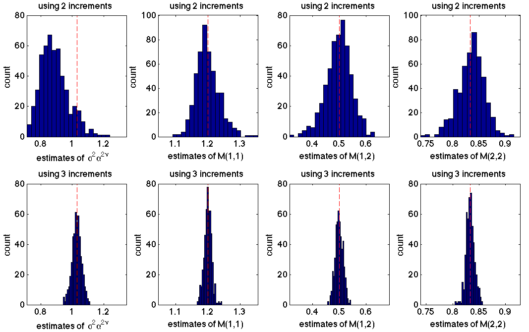
Figure 2: 500 independent simulations of a Matérn random field with $\sigma=1.5$, $\alpha=0.8$, $\nu=1.75$, $M(1,1)=1.2$, $M(1,2)=0.5$, $M(2,1)=0$ and $M(2,2)=1/1.2$ observed on a square grid in $[0,1]^{2}$ with spacing $1/55$. The top row of figures shows the histograms of the estimates of $(\sigma^{2}\alpha^{2\nu},M(1,1),M(1,2),M(2,2))$ using the techniques derived in Section 2.1 based on increments of order 2. The bottom row shows the histograms of the estimates using increments of order 3.

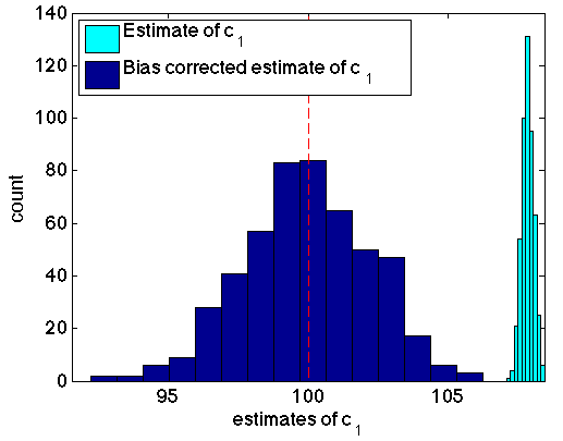
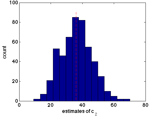
Figure 3: Histograms of the estimates of $c_{1}$ and $c_{2}$ for 500 independent realizations of $\sqrt{c_{1}}\,Y_{1}+\sqrt{c_{2}}\,Y_{2}$ where $c_{1}=100$, $c_{2}=36$ and $Y_{1}$ is independent of $Y_{2}$. The random field $Y_{1}$ has principle irregular term $-|t|^{0.2}$ and $Y_{2}$ has principle irregular term $-|t|^{0.4}$. Each realization is on $[0,1/\sqrt{2})^{2}$ measured at $1000\times 1000$ pixel locations.

Appendix A Proofs

We start with some notation. For a function of two variables $F(\bm{s},\bm{t})$ let $\Delta^{(m,n)}_{\bm{h}}F(\bm{s},\bm{t})\triangleq\Delta^{m}_{\bm{h}}\Delta^{n}_{\bm{h}}F(\bm{s},\bm{t})$ where $\Delta^{m}_{\bm{h}}$ acts on the variable $\bm{s}$ and $\Delta^{n}_{\bm{h}}$ acts on the variable $\bm{t}$. Define $\partial_{\bm{h}}\triangleq\bm{h}\cdot\nabla$ to be the directional derivative in the direction $\bm{h}$ and $\partial_{\bm{h}}^{(m,n)}F(\bm{s},\bm{t})\triangleq\partial^{m}_{\bm{h}}\partial^{n}_{\bm{h}}F(\bm{s},\bm{t})$ where $\partial^{m}_{\bm{h}}$ acts on the variable $\bm{s}$ and $\partial^{n}_{\bm{h}}$ acts on $\bm{t}$.

Let $f(\xi),g(\xi)$ be real valued functions defined on some set $\Xi$ and let $\Xi^{\prime}\subset\Xi$. We write $f(\xi)\lesssim g(\xi)$ for all $\xi\in\Xi^{\prime}$ if there there exists a positive constant $c>0$ such that $|f(\xi)|\leq c\,g(\xi)$ for all $\xi\in\Xi^{\prime}$. Notice that this definition also works for a sequence of functions $f_{n},g_{n}$ by considering the variable $n$ as an argument and replacing $\Xi$ by $\Xi\times\mathbb{N}$.

Proof of Lemma 1.

We suppose $\sigma=\alpha=1$ and $M$ is the identity matrix, then rescale for the general case. First note two immediate facts about the $m^{\text{th}}$ directional increment operator $\Delta_{\bm{h}/n}^{m}$: for any function $f\colon\mathbb{R}^{d}\rightarrow\mathbb{R}$ the $m^{\text{th}}$-increment of $f$ can be computed $\Delta_{\bm{h}/n}^{m}f(\bm{t})=\sum_{i=0}^{m}d_{i}f(\bm{t}+i\bm{h}/n)$ where $d_{i}=(-1)^{m+i}{m\choose i}$; The $m^{\text{th}}$-increment $\Delta_{\bm{h}/n}^{m}$ annihilates monomials of degree less than $m$ so that $\Delta_{\bm{h}/n}^{(m,m)}|\bm{t}-\bm{s}|^{2k}=0$ for all $k=0,\ldots,m-1$. Therefore, by the expansions given on page 375 of [1] we have

$$\Delta_{\bm{h}/n}^{(m,m)}K(|\bm{s}-\bm{t}|)=\Delta_{\bm{h}/n}^{(m,m)}\Bigl{\{}G_{\nu}(|\bm{s}-\bm{t}|)-\nu G_{\nu+1}(|\bm{s}-\bm{t}|)+r(|\bm{s}-\bm{t}|)\Bigr{\}}$$

where $r(\epsilon)=o(\epsilon^{2\nu+2})$ as $\epsilon\rightarrow 0$. Now for a fixed $\bm{t}_{0}\in\mathbb{R}^{d}$

$$\mathsf{E}(\Delta_{\bm{h}/n}^{m}Y(\bm{t}_{0}))^{2}=\Delta_{\bm{h}/n}^{(m,m)}\Bigl{\{}K(|\bm{s}-\bm{t}|)\Bigr{\}}\Bigr{|}_{\bm{s},\bm{t}=\bm{t}_{0}}=\mathcal{I}_{1}+\mathcal{I}_{2}+\mathcal{I}_{3}$$

where

$$\mathcal{I}_{1} \triangleq\Delta_{\bm{h}/n}^{(m,m)}\Bigl{\{}G_{\nu}(|\bm{s}-\bm{t}|)\Bigr{\}}\Bigr{|}_{\bm{s},\bm{t}=\bm{t}_{0}}=\sum_{ij}d_{i}d_{j}G_{\nu}(|(i-j)\bm{h}/n|)$$ (18)

$$\mathcal{I}_{2} \triangleq\Delta_{\bm{h}/n}^{(m,m)}\Bigl{\{}(-\nu)G_{\nu+1}(|\bm{s}-\bm{t}|)\Bigr{\}}\Bigr{|}_{\bm{s},\bm{t}=\bm{t}_{0}}=\sum_{ij}d_{i}d_{j}(-\nu)G_{\nu+1}(|(i-j)\bm{h}/n|)$$ (19)

$$\mathcal{I}_{3} \triangleq\Delta_{\bm{h}/n}^{(m,m)}\Bigl{\{}r(|\bm{s}-\bm{t}|))\Bigr{\}}\Bigr{|}_{\bm{s},\bm{t}=\bm{t}_{0}}=\sum_{ij}d_{i}d_{j}r(|(i-j)\bm{h}/n|)$$ (20)

Notice that $\sum_{ij}d_{i}d_{j}G_{\nu}(|(i-j)\bm{h}/n|)=|\bm{h}/n|^{2\nu}\sum_{ij}d_{i}d_{j}G_{\nu}(|i-j|)$. This is obviously true with $\nu\not\in\mathbb{Z}$. It also holds when $\nu\in\mathbb{Z}$ since

$$G_{\nu}(|(i-j)\bm{h}/n|)=|\bm{h}/n|^{2\nu}\bigl{(}G_{\nu}(|i-j|)+|i-j|^{2\nu}\log|\bm{h}/n|\bigr{)}$$ (21)

and $\sum_{ij}d_{i}d_{j}|i-j|^{2\nu}=0$ (since $\nu\in\mathbb{Z}$ and $m>\nu$). Similar arguments can be applied to $G_{\nu+1}$ when $m>\nu+1$ which gives $\mathcal{I}_{1}+\mathcal{I}_{2}=\frac{a_{\nu}^{m}}{n^{2\nu}}+\frac{b_{\nu}^{m}}{n^{2\nu+2}}$. Finally, notice that $r(\epsilon)=o(\epsilon^{2\nu+2})$ implies that $\mathcal{I}_{3}=o(n^{-2\nu-2})$. This establishes the claim when $\sigma=\alpha=1$ and $M$ is the identity matrix. The general result when $\sigma,\nu>0$ and $M\in GL(d,\mathbb{R})$ is then established by an easy rescaling argument (using equation (21) when $\nu\in\mathbb{Z}$). ∎

Lemma 2.

For $\nu>0$, let $a^{m}_{\nu}$ be defined by (9) and $b^{m}_{\nu}$ be defined by (10). If $m>\nu$ then $a^{m}_{\nu}\neq 0$. If $m>\nu+1$ then $b^{m}_{\nu}\neq 0$. Finally, there exits $p,q>\nu+1$ such that $b^{p}_{\nu}-\frac{a^{p}_{\nu}}{a^{q}_{\nu}}b^{q}_{\nu}\neq 0$.

Proof.

Notice first that $a_{\nu}^{m}\propto\text{var}(\Delta_{1}^{m}Z_{\nu})>0$ where $Z_{\nu}$ is an intrinsic random function on $\mathbb{R}$ observed on $\mathbb{Z}$ with generalized covariance $G_{\nu}$ (since $\Delta_{1}^{m}$ annihilates polynomials of order $m-1$, and $m>\nu$, see [28]). The same reasoning establishes that $-b_{\nu}^{m}\propto\text{var}(\Delta_{1}^{m}Z_{\nu+1})>0$ when $m>\nu+1$.

For the last part of the lemma we show that there exists $p,q>\nu+1$ such that

$$\frac{\text{var}(\Delta_{1}^{p}Z_{\nu})}{\text{var}(\Delta_{1}^{q}Z_{\nu})}\neq\frac{\text{var}(\Delta_{1}^{p}Z_{\nu+1})}{\text{var}(\Delta_{1}^{q}Z_{\nu+1})}.$$

We will argue by contradiction and suppose that for all $k>0$,

$$\frac{\text{var}(\Delta_{1}^{q+k}Z_{\nu})}{\text{var}(\Delta_{1}^{q}Z_{\nu})}=\frac{\text{var}(\Delta_{1}^{q+k}Z_{\nu+1})}{\text{var}(\Delta_{1}^{q}Z_{\nu+1})}.$$ (22)

By a spectral representation of $G_{\nu}$ (see [28] page 36) and an easy induction establishes that $\text{var}(\Delta_{1}^{q+k}Z_{\nu})=\int|e^{iw}-1|^{2q+2k}|w|^{-2\nu-1}\,dw$ and $\text{var}(\Delta_{1}^{q+k}Z_{\nu+1})=\int|e^{iw}-1|^{2q+2k}|w|^{-2\nu-3}\,dw$. Notice also that $|e^{iw}-1|^{2}=2-2\cos\,w$. Let $F_{\nu}$ and $F_{\nu+1}$ be two probability measures on $\mathbb{R}$ defined by

$$F_{\nu}(B) \triangleq\frac{1}{\text{var}(\Delta_{1}^{q}Z_{\nu})}\int_{B}(2-2\cos\,w)^{q}|w|^{-2\nu-1}\,dw$$

$$F_{\nu+1}(B) \triangleq\frac{1}{\text{var}(\Delta_{1}^{q}Z_{\nu+1})}\int_{B}(2-2\cos\,w)^{q}|w|^{-2\nu-3}\,dw.$$

Our assumption (22) then becomes

$$\int(2-2\cos\,w)^{k}dF_{\nu}(w)=\int(2-2\cos\,w)^{k}dF_{\nu+1}(w),$$ (23)

for all $k>0$. Notice that the variances $\text{var}(\Delta_{1}^{q}Z_{\nu})$ and $\text{var}(\Delta_{1}^{q}Z_{\nu+1})$ serve as the normalizing constants so that $F_{\nu}$ and $F_{\nu+1}$ have total mass one. In what follows we show that the normalizing constants satisfy both $\text{var}(\Delta_{1}^{q}Z_{\nu})>\text{var}(\Delta_{1}^{q}Z_{\nu+1})$ and $\text{var}(\Delta_{1}^{q}Z_{\nu})<\text{var}(\Delta_{1}^{q}Z_{\nu+1})$ to establish the desired contradiction.

By the equalities in (23), the random variables $2(1-\cos W_{\nu})$ and $2(1-\cos W_{\nu+1})$ have the same moments when $W_{\nu}\sim F_{\nu}$ and $W_{\nu+1}\sim F_{\nu+1}$. In addition, $0\leq 2(1-\cos W_{\nu})\leq 4$ and $0\leq 2(1-\cos W_{\nu+1})\leq 4$ so that the moment generating functions are both finite in a non-empty radius of the origin. Therefore $2(1-\cos W_{\nu})\overset{\mathcal{L}}{=}2(1-\cos W_{\nu+1})$, where $\overset{\mathcal{L}}{=}$ denotes equality in law. This gives $\mathsf{P}(\cos W_{\nu}<0)=\mathsf{P}(\cos W_{\nu+1}<0)$, for example. However

$$\mathsf{P}(\cos W_{\nu}<0) =\frac{1}{\text{var}(\Delta_{1}^{q}Z_{\nu})}\int\bm{1}_{\{\cos w<0\}}(2-2\cos w)^{q}|w|^{-2\nu-1}dw$$

$$>\frac{1}{\text{var}(\Delta_{1}^{q}Z_{\nu})}\int\bm{1}_{\{\cos w<0\}}(2-2\cos w)^{q}|w|^{-2\nu-3}dw,$$

by the fact that $\cos w<0\Rightarrow|w|>\pi/2$. Therefore

$$\text{var}(\Delta_{1}^{q}Z_{\nu+1})<\text{var}(\Delta_{1}^{q}Z_{\nu}).$$ (24)

To show the contradicting inequality let’s start by computing the density of these two random variables. The idea is to show that the non-normalized (i.e.​ without the term $\text{var}(\Delta_{1}^{q}Z_{\nu})$) density of $2(1-\cos W_{\nu})$ is strictly smaller than the non-normalized density of $2(1-\cos W_{\nu+1})$ in a positive neighborhood of $0$. In particular, the density of $2(1-\cos W_{\nu})$ can be written as $2\sum_{k=1}^{\infty}f_{W_{\nu}}(g_{k}(x))|g_{k}(x)^{\prime}|$ where the $g_{k}$’s are the different positive branches of the inverse $\cos^{-1}(1-x/2)$ and $f_{W_{\nu}}(w)\triangleq(2-2\cos w)^{q}|w|^{-2\nu-1}/\text{var}(\Delta_{1}^{q}Z_{\nu})$ is the density of $W_{\nu}$. This simplifies to

$$\frac{2x^{q}}{\text{var}(\Delta_{1}^{q}Z_{\nu})}\sum_{k=1}^{\infty}\frac{|g_{k}(x)^{\prime}|}{|g_{k}(x)|^{2\nu+1}}=\frac{2x^{q}}{\text{var}(\Delta^{q}Z_{\nu})\sqrt{x-x^{2}/4}}\sum_{k=1}^{\infty}{|g_{k}(x)|^{-2\nu-1}}$$

for $0<x<4$. Notice that $g_{1}(x)\sim\sqrt{x}$ as $x\rightarrow 0$ and $g_{k}(x)\sim 2\pi\lfloor k/2\rfloor$ as $x\rightarrow 0$ for all $k>1$. Therefore the term $g_{1}$ dominates the sum when $x$ is small. In particular for all $x>0$ sufficiently small we have

$$f_{2-2\cos W_{\nu}}(x) <\frac{2x^{q}}{\text{var}(\Delta_{1}^{q}Z_{\nu})\sqrt{x-x^{2}/4}}\sum_{k=1}^{\infty}{|g_{k}(x)|^{-2\nu-3}}$$ (25)

$$=\frac{\text{var}(\Delta_{1}^{q}Z_{\nu+1})}{\text{var}(\Delta_{1}^{q}Z_{\nu})}f_{2-2\cos W_{\nu+1}}(x).$$ (26)

Since $f_{2-2\cos W_{\nu}}(x)$ and $f_{2-2\cos W_{\nu+1}}(x)$ have the same integrate integrals over Borel subsets of $(0,4)$, we must have $\text{var}(\Delta_{1}^{q}Z_{\nu+1})>\text{var}(\Delta_{1}^{q}Z_{\nu})$. This contradicts (24) and therefore establishes the lemma. ∎

Lemma 3.

For any $\nu>0$, $T>0$,

$$\Bigl{|}\frac{d^{p}}{dt^{p}}t^{\nu/2}\mathcal{K}_{\nu}(\sqrt{t})\Bigr{|}\lesssim\begin{cases}1,&\text{when $p<\nu$;}\\ |\log t|,&\text{when $p=\nu$;}\\ t^{\nu-p},&\text{when $p>\nu$;}\end{cases}$$

as $t$ ranges in the interval $(0,T)$ where $\mathcal{K}_{\nu}$ is the modified Bessel function of the second kind of order $\nu$.

Proof.

Using the expansions for $\mathcal{K}_{\nu}$ found in [1] (page 375) we can write

$$t^{\nu/2}\mathcal{K}_{\nu}(\sqrt{t}) =\begin{cases}F_{1}(t)+t^{\nu}\log(t)F_{3}(t);&\text{when $\nu=0,1,2,\ldots$}\\ F_{4}(t)+t^{\nu}F_{5}(t);&\text{otherwise}\end{cases}$$ (27)

where the $F_{j}(t)$’s are of the form $\sum_{k=0}^{\infty}c_{k}t^{k}$ where the $c_{k}$’s decay fast enough so that the series converges absolutely for all $t\in(0,\infty)$ and all it’s derivatives exist and are bounded on $(0,T)$. This immediately establishes that when $p<\nu$, $\bigl{|}\frac{d^{p}}{dt^{p}}t^{\nu/2}\mathcal{K}_{\nu}(\sqrt{t})\bigr{|}\lesssim 1$ for all $t\in(0,T)$ since both $\frac{d^{p}}{dt^{p}}(t^{\nu})$ and $\frac{d^{p}}{dt^{p}}(t^{\nu}\log t)$ are continuous and bounded on $(0,T)$.

When $p>\nu$ and $\nu\not\in\mathbb{Z}$ we have that $t^{\nu}\lesssim\frac{d}{dt}(t^{\nu})\lesssim\cdots\lesssim\frac{d^{p}}{dt^{p}}(t^{\nu})\lesssim t^{\nu-p}$ as $t$ ranges in the bounded interval $(0,T)$. Similarly, when $p>\nu$ and $\nu\in\mathbb{Z}$ we have

$$t^{\nu}\log t\lesssim\frac{d}{dt}(t^{\nu}\log t)\lesssim\cdots\lesssim\frac{d^{p}}{dt^{p}}(t^{\nu}\log t)\lesssim t^{\nu-p}.$$

Finally, when $p=\nu$, $\frac{d^{p}}{dt^{p}}t^{\nu}\log t\propto\log t+c_{p}$. The lemma now follows by equation (27) and the fact that the derivative of a product satisfies $(fg)^{(p)}=\sum_{k=0}^{p}{p\choose k}f^{(p)}g^{(p-k)}$.

∎

Lemma 4.

Suppose $K(t)$ is the isotropic Matérn autocovariance function defined in (6) for fixed parameters $\sigma,\alpha,\nu>0$. Then for any integer $m>\nu$, nonzero vector $\bm{h}\in\mathbb{R}^{d}$, matrix $M\in GL(d,\mathbb{R})$ and bounded set $\Omega\subset\mathbb{R}^{d}$

$$\bigl{|}\partial_{\bm{h}}^{(m,m)}\bigl{[}K(|M\bm{s}-M\bm{t}|)\bigr{]}\bigr{|}\lesssim|\bm{s}-\bm{t}|^{2\nu-2m}$$ (28)

for all $\bm{s},\bm{t}\in\Omega$ such that $\bm{s}\neq\bm{t}$.

Proof.

First notice that it is sufficient to show the claim when $M$ is the identity matrix and $\alpha=1$ (extending to general $M$ and $\alpha$ follows by the chain rule for derivatives). Define $K_{sq}(t)\triangleq K(\sqrt{t})$ and $F(\bm{s},\bm{t})\triangleq|\bm{s}-\bm{t}|^{2}$ so that $\partial_{\bm{h}}^{(m,m)}\bigl{[}K(|\bm{s}-\bm{t}|)\bigr{]}=\partial_{\bm{h}}^{(m,m)}\bigl{[}K_{sq}(F(\bm{s},\bm{t}))\bigr{]}$. Also let $\partial_{\bm{h}}^{*}$ denote a generic directional derivative on either the variable $\bm{s}$ or $\bm{t}$. By generic I mean that $(\partial_{\bm{h}}^{*})^{k}F$ denotes $\partial_{\bm{h}}^{(i,j)}F$ for some $i+j=k$ and $(\partial_{h}^{*}F)^{k}=\partial_{\bm{h}}^{*}F\cdots\partial_{\bm{h}}^{*}F$ where each $\partial_{\bm{h}}^{*}$ could be with respect to $\bm{s}$ or $\bm{t}$. Now by successive application of the directional derivatives $\partial_{\bm{h}}^{*}$ we get that

$$\partial_{\bm{h}}^{(m,m)}\bigl{[}K_{sq}(F(\bm{s},\bm{t}))\bigr{]}=\sum_{i=1}^{2m}\sum_{\begin{subarray}{c}0\leq j\leq i\\ j+i\leq 2m\end{subarray}}K_{sq}^{(i)}(F(\bm{s},\bm{t}))(\partial_{\bm{h}}^{*}F(\bm{s},\bm{t}))^{i-j}B_{ij}$$ (29)

where each $B_{ij}$ is uniformly bounded on $\Omega^{2}$. The functions $B_{ij}$ are uniformly bounded by the nice fact that $(\partial_{\bm{h}}^{*})^{k}F(\bm{s},\bm{t})\lesssim 1$ on $\Omega^{2}$ when $k\geq 2$.

We will bound the terms of the sum (29) when $i<\nu$, $i>\nu$, and $i=\nu$ separately. Notice first that since $i\geq j$ we have that

$$\bigl{|}\partial_{\bm{h}}^{*}F(\bm{s},\bm{t})\bigr{|}^{i-j} \lesssim|\bm{s}-\bm{t}|^{i-j},\quad\text{for all $\bm{s},\bm{t}\in\Omega$.}$$ (30)

This implies, by Lemma 3, that the terms in the sum (29), for which $i<\nu$, are bounded. When $i>\nu$

$$|K_{sq}^{(i)}(F(\bm{s},\bm{t}))(\partial_{\bm{h}}^{*}F(\bm{s},\bm{t}))^{i-j}B_{ij}| \lesssim|F(\bm{s},\bm{t})|^{\nu-i}|\bm{s}-\bm{t}|^{i-j},\quad\text{by (\ref{uuu}) and Lemma \ref{ksqrt}}$$

$$=|\bm{s}-\bm{t}|^{2\nu-(i+j)}$$

$$\lesssim|\bm{s}-\bm{t}|^{2\nu-2m},\quad\text{since $i+j\leq 2m$,}$$

where the inequality holds for all $\bm{s},\bm{t}\in\Omega$ such that $|\bm{s}-\bm{t}|>0$ (note that we use the fact that $\Omega$ is bounded implies $|\bm{s}-\bm{t}|<T$ for some $T$). For the last case, $i=\nu$, a similar argument establishes

$$|K_{sq}^{(i)}(F(\bm{s},\bm{t}))(\partial_{\bm{h}}^{*}F(\bm{s},\bm{t}))^{i-j}B_{ij}| \lesssim|\bm{s}-\bm{t}|^{i-j}|\log F(\bm{s},\bm{t})|$$

$$\lesssim|\bm{s}-\bm{t}|^{2\nu-2m}$$

for all $\bm{s},\bm{t}\in\Omega$ such that $|\bm{s}-\bm{t}|>0$. Therefore $\partial_{\bm{h}}^{(m,m)}\bigl{[}K_{sq}(F(\bm{s},\bm{t}))\bigr{]}\lesssim|\bm{s}-\bm{t}|^{2\nu-2m}$ for all $\bm{s},\bm{t}\in\Omega$ such that $\bm{s}\neq\bm{t}$. ∎

Lemma 5.

Let $\bm{h}$ be a nonzero vector in $\mathbb{R}^{d}$, $\nu>0$ and $H$ be the $d\times m$ matrix defined by

$$H\triangleq\underbrace{(\bm{h},\cdots,\bm{h})}_{\text{$m$ columns}}.$$ (31)

If $m$ is a positive integer greater than $\nu$ then

$$\sup_{\bm{\xi,\eta}\in[0,1]^{m}}|\bm{i-j}+H(\bm{\xi}-\bm{\eta})/n|^{2\nu-2m}\lesssim|\bm{i-j}|^{2\nu-2m}$$

for all positive integers $n$ and $\bm{i},\bm{j}\in\Omega_{n}$ such that $|\bm{i}-\bm{j}|>|(m+1)\bm{h}/n|$.

Proof.

First notice that $\sup_{\bm{\xi,\eta}\in[0,1]^{m}}|\bm{i-j}+H(\bm{\xi}-\bm{\eta})/n|^{2\nu-2m}=\sup_{-1\leq\tau\leq 1}|\bm{i-j}+m\bm{h}\tau/n|^{2\nu-2m}$. Now for any $-1\leq\tau\leq 1$, positive integer $n$ and $\bm{i},\bm{j}\in\Omega_{n}$ such that $|\bm{i}-\bm{j}|>|(m+1)\bm{h}/n|$, we have

$$|\bm{i}-\bm{j}+m\bm{h}\tau/n| \geq|\bm{i}-\bm{j}|-m|\tau||\bm{h}|/n$$

$$\geq|\bm{i}-\bm{j}|-|\bm{i}-\bm{j}|\frac{m}{m+1}.$$

The last line follows from the assumption that $|\bm{i}-\bm{j}|>(m+1)|\bm{h}|/n$ which implies $\frac{m}{m+1}|\bm{i}-\bm{j}|>m|\bm{h}|/n$. Therefore

$$\sup_{\bm{\xi,\eta}\in[0,1]^{m}}\bigl{|}\bm{i-j}+H(\bm{\xi}-\bm{\eta})/n\bigr{|}^{2\nu-2m}\leq\Bigl{(}1-\frac{m}{m+1}\Bigr{)}^{2\nu-2m}|\bm{i-j}|^{2\nu-2m}.$$

∎

Lemma 6.

Let $Y$ be a mean zero, geometric anisotropic $d$-dimensional Matérn Gaussian random field with parameters $(\sigma,\alpha,\nu,M)$ and let $\Omega$ be a bounded, open subset of $\mathbb{R}^{d}$. Fix a positive integer $m>\nu$ and a non-zero vector $\bm{h}\in\mathbb{R}^{d}$. Let $\Sigma$ to be the covariance matrix of the increments $\Delta_{\bm{h}/n}^{m}Y(\bm{i})$ as $\bm{i}$ ranges in the set $\bm{i}\in\Omega_{n}$ so that

$$\Sigma(\bm{i},\bm{j})\triangleq\mathsf{E}\bigl{(}\Delta_{\bm{h}/n}^{m}Y(\bm{i})\Delta_{\bm{h}/n}^{m}Y(\bm{j})\bigr{)}$$ (32)

for all $\bm{i},\bm{j}\in\Omega_{n}$. Then there exists an $N>0$ such that

$$|\Sigma(\bm{i},\bm{j})|\lesssim n^{-2m}|\bm{i}-\bm{j}|^{2\nu-2m}$$ (33)

for all $n>N$, and $\bm{i},\bm{j}\in\Omega_{n}$ such that $|\bm{i}-\bm{j}|>|(m+1)\bm{h}/n|$. Moreover,

$$|\Sigma(\bm{i},\bm{j})|\lesssim n^{-2\nu}$$ (34)

for all $n>N$ and $\bm{i},\bm{j}\in\Omega_{n}$ such that $|\bm{i}-\bm{j}|\leq|(m+1)\bm{h}/n|$.

Proof.

First notice that $\Sigma(\bm{i},\bm{j})=\mathsf{E}\Delta_{\bm{h}/n}^{m}Y(\bm{i})\Delta_{\bm{h}/n}^{m}Y(\bm{j})=\Delta_{\bm{h}/n}^{(m,m)}K(|M(\bm{i}-\bm{j})|)$ where $K$ is the isotropic Matérn autocovariance function defined in (6). To simplify the notation let $F(\bm{i},\bm{j})\triangleq K(|M(\bm{i}-\bm{j})|)$ and $H$ be the $d$ by $m$ matrix defined in (31). An induction argument on $m$ establishes that when $|\bm{i}-\bm{j}|>(m+1)|\bm{h}|/n$ we can express directional increments as integrals of directional derivatives so that

$$\Delta_{\bm{h}/n}^{(m,m)}F(\bm{i},\bm{j})=\frac{1}{n^{2m}}\int_{\bm{\xi},\bm{\eta}\in[0,1]^{m}}(\partial_{\bm{h}}^{(m,m)}F)(\bm{i}+H\bm{\xi}/n,\bm{j}+H\bm{\eta}/n)d\bm{\xi}d\bm{\eta}.$$

Therefore

$$|\Sigma(\bm{i},\bm{j})| \lesssim\frac{1}{n^{2m}}\int_{\bm{\xi},\bm{\eta}\in[0,1]^{m}}\bigl{|}(\partial_{\bm{h}}^{(m,m)}F)(\bm{i}+H\bm{\xi}/n,\bm{j}+H\bm{\eta}/n)\bigr{|}d\bm{\xi}d\bm{\eta}$$

$$\lesssim\frac{1}{n^{2m}}\int_{\bm{\xi},\bm{\eta}\in[0,1]^{m}}\bigl{|}\bm{i-j}+H(\bm{\xi}-\bm{\eta})/n\bigr{|}^{2\nu-2m}d\bm{\xi}d\bm{\eta},\quad\text{by Lemma \ref{boundonderiv}}$$

$$\lesssim\frac{1}{n^{2m}}\sup_{\bm{\xi,\eta}\in[0,1]^{m}}\bigl{|}\bm{i-j}+H(\bm{\xi}-\bm{\eta})/n\bigr{|}^{2\nu-2m}$$

$$\lesssim\frac{1}{n^{2m}}\bigl{|}\bm{i-j}\bigr{|}^{2\nu-2m}\!,\quad\text{by Lemma \ref{suprem}}$$

for all $n>N$, $\bm{i},\bm{j}\in\Omega_{n}$ such that $|\bm{i}-\bm{j}|>|(m+1)\bm{h}/n|$. On the other hand when $|\bm{i}-\bm{j}|\leq|(m+1)\bm{h}/n|$

$$|\Sigma(\bm{i},\bm{j})| \leq\sqrt{\mathsf{E}(\Delta_{\bm{h}/n}^{m}Y(\bm{i}))^{2}}\sqrt{\mathsf{E}(\Delta_{\bm{h}/n}^{m}Y(\bm{j}))^{2}}\lesssim n^{-2\nu}$$ (35)

where the last inequality is by Lemma 1. Actually, a direct application of Lemma 1 only establishes (35) when $m>\nu+1$. However, a small adjustment of the proof of Lemma 1 establishes that $\mathsf{E}(\Delta_{\bm{h}/n}^{m}Y(\bm{t}))^{2}=\frac{a_{\nu}^{m}}{n^{2\nu}}+o(n^{-2\nu})$ as $n\rightarrow\infty$ when $m>\nu$. This is then is sufficient to establish (35). ∎

Lemma 7.

Let $\Sigma_{\text{abs}}$ be the component-wise absolute value of the covariance matrix $\Sigma$ (defined in (32)). Then under the same assumptions as in Lemma 6, there exits an $N>0$ such that

$$\|\Sigma_{abs}\|_{2}\lesssim n^{-2\nu}+c\,{n^{d-2m}}\int_{1/n}^{1}r^{2\nu-2m+d-1}dr.$$

for all $n>N$, where $c$ is a constant and $\|\cdot\|_{2}$ is the spectral norm.

Proof.

First note that by symmetry, $\|\Sigma_{abs}\|_{2}\leq\sqrt{\|\Sigma_{abs}\|_{1}\|\Sigma_{abs}\|_{\infty}}=\|\Sigma_{abs}\|_{\infty}$, where $\|\Sigma_{abs}\|_{\infty}$ is the maximum of the $\ell_{1}$ row norms and $\|\Sigma_{abs}\|_{1}$ is the maximum of the $\ell_{1}$ column norms. To bound the $\ell_{1}$ row norms, we bound the terms of the sum when $|\bm{i}-\bm{j}|>(m+1)|\bm{h}|/n$ and $|\bm{i}-\bm{j}|\leq(m+1)|\bm{h}|/n$ separately. For the off-diagonal terms we use Lemma 6 to ensure the existence of an $N>0$ such that for all $n>N$

$$\max_{\bm{i}\in\Omega_{n}}\sum_{\begin{subarray}{c}\bm{j}\in\Omega_{n}\\ |\bm{i}-\bm{j}|>(m+1)|\bm{h}|/n\end{subarray}}|\Sigma(\bm{i},\bm{j})| \lesssim\max_{\bm{i}\in\Omega_{n}}\sum_{\begin{subarray}{c}\bm{j}\in\Omega_{n}\\ |\bm{i}-\bm{j}|>(m+1)|\bm{h}|/n\end{subarray}}n^{-2m}|\bm{i}-\bm{j}|^{2\nu-2m}$$ (36)

$$\lesssim{n^{d-2m}}\int_{1/n}^{1}r^{2\nu-2m+d-1}dr.$$ (37)

The last inequality, (37), follows by the fact that for any constant $a>0$ and open set $\Theta\subset\mathbb{R}^{d}$ which is bounded and contains the origin, one has

$$\sum_{\begin{subarray}{c}\bm{i}\in\Theta\cap\{\mathbb{Z}^{d}/n\}\\ |\bm{i}|>a/n\end{subarray}}n^{-d}|\bm{i}|^{\beta}\lesssim\int_{1/n}^{1}r^{\beta+d-1}dr$$ (38)

as $n\rightarrow\infty$ (for details see [3], Lemma 3, page 41). In addition, by Lemma 6

$$\max_{\bm{i}\in\Omega_{n}}\sum_{\begin{subarray}{c}\bm{j}\in\Omega_{n}\\ |\bm{i}-\bm{j}|\leq(m+1)|\bm{h}|/n\end{subarray}}|\Sigma(\bm{i},\bm{j})| \lesssim n^{-2\nu}$$ (39)

for all $n>N$. This establishes the proof by noticing that the sum of the last terms in (37) and (39) bound $\|\Sigma_{abs}\|_{\infty}$. ∎

Lemma 8.

Under the same assumptions as in Lemma 6 there exits an $N>0$ such that

$$\|\Sigma\|_{F}^{2}\lesssim{n^{d-4\nu}}+c\,n^{2d-4m}\int_{1/n}^{1}r^{4\nu-4m+d-1}dr$$

for all $n>N$ where $c$ is a constant and $\|\cdot\|_{F}$ denotes the Frobenious matrix norm.

Proof.

First note that $\|\Sigma\|_{F}^{2}=\sum_{\bm{i},\bm{j}\in\Omega_{n}}|\Sigma(\bm{i},\bm{j})|^{2}$. As in the proof of Lemma 8 we bound the near-diagonal terms of $\Sigma$ separately from the off-diagonal terms. By Lemma 6 there exists an $N>0$ such that

$$\sum_{\begin{subarray}{c}\bm{i},\bm{j}\in\Omega_{n}\\ |\bm{i}-\bm{j}|>(m+1)|\bm{h}|/n\end{subarray}}|\Sigma(\bm{i},\bm{j})|^{2} \lesssim n^{2d-4m}\sum_{\begin{subarray}{c}\bm{i},\bm{j}\in\Omega_{n}\\ |\bm{i}-\bm{j}|>(m+1)|\bm{h}|/n\end{subarray}}n^{-2d}|\bm{i}-\bm{j}|^{4\nu-4m}$$ (40)

$$\lesssim n^{2d-4m}\int_{1/n}^{1}r^{4\nu-4m+d-1}dr$$ (41)

for all $n>N$. Notice that the last inequality is a slight variation on (38). For the near diagonal terms we also use Lemma 6 to get

$$\sum_{\begin{subarray}{c}\bm{i},\bm{j}\in\Omega_{n}\\ |\bm{i}-\bm{j}|\leq(m+1)|\bm{h}|/n\end{subarray}}|\Sigma(\bm{i},\bm{j})|^{2} \lesssim n^{d}n^{-4\nu}.$$ (42)

Adding (41) and (42) establishes the lemma. ∎

Proof of Theorem 1.

Define the random vector $\Delta Y$ to be the vector of $m$-increments, the components of which are indexed by $\Omega_{n}$ (in any order), so that

$$\Delta Y\triangleq\underbrace{\bigl{(}\ldots,\Delta_{\bm{h}/n}^{m}Y(\bm{j}),\ldots\bigr{)}}_{\text{terms are indexed by $\bm{j}\in\Omega_{n}$}}.$$ (43)

Now we can write $Q_{n}^{m}=\frac{n^{2\nu}}{\#\Omega_{n}}\Delta Y\Delta Y^{T}=\frac{n^{2\nu}}{\#\Omega_{n}}W\Sigma W^{T}$, where $W\sim\mathcal{N}(\bm{0},I)$ (note that $\Sigma$ is defined in (32)). Therefore $\text{var}\,Q_{n}^{m}=2\frac{n^{4\nu}}{(\#\Omega)^{2}}\|\Sigma\|^{2}_{F}$ and by Lemma 8

$$\frac{n^{4\nu}}{(\#\Omega)^{2}}\|\Sigma\|^{2}_{F} \lesssim n^{-d}+c\,n^{4\nu-4m}\int_{1/n}^{1}r^{4\nu-4m+d-1}dr$$

$$\lesssim\begin{cases}n^{4(\nu-m)},&\text{if $4(\nu-m)>-d$;}\\ n^{-d}\log n,&\text{if $4(\nu-m)=-d$;}\\ n^{-d},&\text{if $4(\nu-m)<-d$}\end{cases}$$

for all sufficiently large $n$. This establishes the variance rates.

For the almost sure convergence result let $\tilde{\Sigma}\triangleq\frac{n^{2\nu}}{\#\Omega_{n}}\Sigma_{abs}$ where $\Sigma_{abs}$ is the component-wise absolute value of $\Sigma$. The Hanson and Wright bound in [17] then gives

$$\mathsf{P}(|Q_{n}^{m}-EQ_{n}^{m}|\geq\epsilon)\leq 2\exp\left(-\frac{c_{1}\epsilon}{\|\tilde{\Sigma}\|_{2}}\wedge\frac{c_{2}\epsilon^{2}}{\|\tilde{\Sigma}\|_{F}^{2}}\right)$$ (44)

for all $\epsilon>0$, where $c_{1},c_{2}$ are positive constants not depending on $n$ or $\tilde{\Sigma}$. First notice that by Lemma 7 we get

$$\|\tilde{\Sigma}\|_{2}=\frac{n^{2\nu}}{\#\Omega_{n}}\|\Sigma_{abs}\|_{2} \lesssim n^{-d}+c\,{n^{2\nu-2m}}\int_{1/n}^{1}r^{2\nu-2m+d-1}dr$$ (45)

$$\lesssim\begin{cases}n^{2(\nu-m)},&\text{if $2(\nu-m)>-d$;}\\ n^{-d}\log n,&\text{if $2(\nu-m)=-d$;}\\ n^{-d},&\text{if $2(\nu-m)<-d$.}\end{cases}$$ (46)

for sufficiently large $n$. Also notice that this implies that $\|\tilde{\Sigma}\|_{F}^{2}\lesssim\|\tilde{\Sigma}\|_{2}$ for sufficiently large $n$. Therefore for sufficiently small $\epsilon$, $\mathsf{P}(|Q_{n}^{m}-EQ_{n}^{m}|\geq\epsilon)\leq 2\exp\left(-c_{2}\epsilon^{2}/\|\tilde{\Sigma}\|_{2}\right)$. Now the rates in (46) and the Borel-Cantelli Lemma are sufficient to establish that $Q_{n}^{m}-\mathsf{E}Q_{n}^{m}\rightarrow 0$, with probability one as $n\rightarrow\infty$. By Lemma 1, $\mathsf{E}Q_{n}^{m}\rightarrow a_{\nu}^{m}$ (a slight adjustment also proves the case when $m>\nu$ rather than $m>\nu+1$) which establishes the theorem. ∎

Proof of Theorem 2.

First notice that when $p,q>\nu+1$

$$\mathsf{E}n^{2}\left[Q^{p}_{n}-\frac{a^{p}_{\nu}}{a^{q}_{\nu}}Q^{q}_{n}\right]\rightarrow\left[b^{p}_{\nu}-\frac{a^{p}_{\nu}}{a^{q}_{\nu}}b^{q}_{\nu}\right]$$ (47)

as $n\rightarrow\infty$ by Lemma 1. To get almost sure convergence notice

$$\mathsf{P}\Bigl{(}n^{2}\Bigl{|}\bigr{[}Q^{p}_{n}-\frac{a^{p}_{\nu}}{a^{q}_{\nu}}Q^{q}_{n}\bigr{]} -\mathsf{E}\bigl{[}Q^{p}_{n}-\frac{a^{p}_{\nu}}{a^{q}_{\nu}}Q^{q}_{n}\bigr{]}\Bigr{|}\geq\epsilon\Bigr{)}$$ (48)

$$\leq\mathsf{P}\bigl{(}|[Q^{p}_{n}-\mathsf{E}Q^{p}_{n}|\geq\epsilon/2n^{2}\bigr{)}+\mathsf{P}\bigl{(}|{a^{p}_{\nu}}||Q^{q}_{n}-\mathsf{E}Q^{q}_{n}|\geq|{a^{q}_{\nu}}|\epsilon/2n^{2}\bigr{)}$$ (49)

We can again use the Hanson and Wright bound ([17]) and the rates derived in Theorem 1 to get

$$\mathsf{P}(|Q_{n}^{p}-\mathsf{E}Q_{n}^{p}|\geq\epsilon/2n^{2})\leq 2\exp\left(-c\,n^{-4}\epsilon^{2}/\|\tilde{\Sigma}\|_{2}\right)$$ (50)

for all sufficiently small $\epsilon>0$ where $c$ is a positive constant that doesn’t depend on $n$ or $\tilde{\Sigma}$. By inspection of the rates in (46) the Borel-Cantelli Lemma can be applied when $4<\min\{2p-2\nu,d\}$ so that $Q_{n}^{p}-EQ_{n}^{p}\rightarrow 0$ with probability one as $n\rightarrow\infty$. A similar result holds for the second term in (49) using the fact that both $a_{\nu}^{p}$ and $a_{\nu}^{q}$ are non-zero by Lemma 2. This, combined with convergence of the expectation in (47), completes the proof. ∎

Proof of Theorem 4.

First notice that for any $p>\delta_{2}/2$

$$\mathsf{E}(\Delta_{\bm{h}/n}^{p}Y(\bm{t}))^{2} =\Delta_{\bm{h}/n}^{(p,p)}\Bigl{\{}c_{1}|\bm{x}-\bm{y}|^{\delta_{1}}+c_{2}|\bm{x}-\bm{y}|^{\delta_{2}}\Bigr{\}}_{\bm{x}=\bm{y}=\bm{t}}$$ (51)

$$=\frac{c_{1}C_{p,\delta_{1}}}{n^{\delta_{1}}}+\frac{c_{2}C_{p,\delta_{2}}}{n^{\delta_{2}}}$$ (52)

where $C_{p,\delta}\triangleq|\bm{h}|^{\delta}\sum_{i,j=0}^{p}(-1)^{i+j}{p\choose i}{p\choose j}|i-j|^{\delta}$. This follows since $Y$ is an intrinsic random function of order $\lfloor\delta_{2}/2\rfloor$ with generalized autocovariance function $c_{1}|\cdot|^{\delta_{1}}+c_{2}|\cdot|^{\delta_{2}}$ and $\Delta_{\bm{h}/n}^{p}$ is an allowable linear combination of order $\lfloor\delta_{2}/2\rfloor$ (see [9]). Now $Q_{n}^{p}$ is defined as in (11) with $\delta_{1}$ in place of $2\nu$ so that

$$Q_{n}^{p}\triangleq\frac{1}{\#\Omega_{n}}\sum_{\bm{j}\in\Omega_{n}}n^{\delta_{1}}(\Delta_{\bm{h}/n}^{p}Y(\bm{j}))^{2}.$$

For any integer $q,p>\delta_{2}/2$ we have that $\mathsf{E}Q_{n}^{p}=c_{1}C_{p,\delta_{1}}+c_{2}C_{p,\delta_{2}}n^{\delta_{1}-\delta_{2}}$ and $n^{\delta_{2}-\delta_{1}}\mathsf{E}\bigl{[}Q_{n}^{p}-\frac{C_{p,\delta_{1}}}{C_{q,\delta_{1}}}Q_{n}^{q}\bigr{]}=c_{2}\bigl{[}C_{p,\delta_{2}}-\frac{C_{p,\delta_{1}}}{C_{q,\delta_{1}}}C_{q,\delta_{2}}\bigr{]}$. By a proof similar to Lemma 2 one can show that for any $p>\delta_{2}/2$ there exists a $q>p$ such that $C_{q,\delta_{1}}\neq 0$ and $C_{p,\delta_{2}}-\frac{C_{p,\delta_{1}}}{C_{q,\delta_{1}}}C_{q,\delta_{2}}\neq 0$ (this uses the fact that $\delta_{1}$, $\delta_{2}$ are not even integers). This motivates the following definition

$$\hat{c}_{1} \triangleq Q_{n}^{p}/C_{p,\delta_{1}}$$ (53)

$$\hat{c}_{2} \triangleq n^{\delta_{2}-\delta_{1}}\frac{Q_{n}^{p}-\frac{C_{p,\delta_{1}}}{C_{q,\delta_{1}}}Q_{n}^{q}}{C_{p,\delta_{2}}-\frac{C_{p,\delta_{1}}}{C_{q,\delta_{1}}}C_{q,\delta_{2}}}.$$ (54)

In what follows we show that $p>\delta_{2}/2$ implies $\hat{c}_{1}\overset{a.s.}{\longrightarrow}c_{1}$ as $n\rightarrow\infty$. Moreover if $2(\delta_{2}-\delta_{1})<\min\{2p-\delta_{1},d\}$ then there exists a $q>p$ such that $\hat{c}_{2}\overset{a.s.}{\longrightarrow}c_{2}$.

We start by letting $\Sigma(\bm{i},\bm{j})\triangleq\mathsf{E}\bigl{(}\Delta_{\bm{h}/n}^{p}Y(\bm{i})\Delta_{\bm{h}/n}^{p}Y(\bm{j})\bigr{)}$ for all $\bm{i},\bm{j}\in\Omega_{n}$ and $\tilde{\Sigma}\triangleq\frac{n^{\delta_{1}}}{\#\Omega_{n}}\Sigma_{abs}$ where $\Sigma_{abs}$ is the component-wise absolute value of $\Sigma$. The Hanson and Wright bound in [17] gives

$$\mathsf{P}(|Q_{n}^{p}-EQ_{n}^{p}|\geq\epsilon)\leq 2\exp\left(-\frac{b_{1}\epsilon}{\|\tilde{\Sigma}\|_{2}}\wedge\frac{b_{2}\epsilon^{2}}{\|\tilde{\Sigma}\|_{F}^{2}}\right)$$ (55)

for all $\epsilon>0$, where $b_{1},b_{2}$ are positive constants not depending on $n$ or $\tilde{\Sigma}$. Later in the proof we will show that when $p>\delta_{2}/2$

$$\|\tilde{\Sigma}\|_{F}^{2}\lesssim\|\tilde{\Sigma}\|_{2}\lesssim\begin{cases}n^{\delta_{1}-2p},&\text{if $0>\delta_{1}-2p>-d$;}\\ n^{-d}\log n,&\text{if $\delta_{1}-2p=-d$;}\\ n^{-d},&\text{if $\delta_{1}-2p<-d$.}\end{cases}$$ (56)

for all sufficiently large $n$. First, however, we show this is sufficient for the almost sure convergence result. Equations (55) and (56) immediately establishes that $\hat{c}_{1}\overset{a.s.}{\longrightarrow}c_{1}$ when $p>\delta_{2}/2$ since $|Q_{n}^{p}-EQ_{n}^{p}|\overset{a.s.}{\longrightarrow}0$ by Borel-Cantelli and $\mathsf{E}\hat{c}_{1}\rightarrow c_{1}$. To see that $\hat{c}_{2}\overset{a.s.}{\longrightarrow}c_{2}$ notice that

$$\mathsf{P}(n^{\delta_{2}-\delta_{1}}|Q_{n}^{p}-EQ_{n}^{p}|\geq\epsilon) \leq 2\exp\left(-\frac{b_{2}\epsilon^{2}}{n^{2(\delta_{2}-\delta_{1})}\|\tilde{\Sigma}\|_{2}}\right)$$ (57)

for all sufficiently small $\epsilon>0$ and sufficiently large $n$. Therefore, by inspection of the rates in (56), one can show that $n^{\delta_{2}-\delta_{1}}|Q_{n}^{p}-EQ_{n}^{p}|\overset{a.s.}{\longrightarrow}0$ whenever $2(\delta_{2}-\delta_{1})<\min\{2p-\delta_{1},d\}$ and $p>\delta_{2}/2$. Since $\mathsf{E}\hat{c}_{2}=c_{2}$, this is sufficient to establish that there exists a $q>p$ such that $\hat{c}_{2}\overset{a.s.}{\longrightarrow}c_{2}$ as $n\rightarrow\infty$ when $0<2(\delta_{2}-\delta_{1})<\min\{2p-\delta_{1},d\}$ and $p>\delta_{2}/2$.

Now to finish the proof we need to establish (56). We start by noticing that for any $p>\delta_{2}/2$ there exists a constant $c>0$ such that

$$\bigl{|}\partial_{\bm{h}}^{(p,p)}\text{cov}(Y(\bm{s}),Y(\bm{t}))\bigr{|} =\bigl{|}\partial_{\bm{h}}^{(p,p)}\bigl{\{}c_{1}|\bm{s}-\bm{t}|^{\delta_{1}}+c_{2}|\bm{s}-\bm{t}|^{\delta_{2}}\bigr{\}}\bigr{|}$$

$$\leq b_{4}|\bm{s}-\bm{t}|^{\delta_{1}-2p}$$

for all $\bm{s},\bm{t}\in\Omega$ such that $\bm{s}\neq\bm{t}$ where $b_{4}$ is a positive constant. Following the proofs of Lemma 6 we can then derive that there exists an $N>0$ such that for any $p>\delta_{2}/2$

$$|\Sigma(\bm{i},\bm{j})|\lesssim n^{-2p}|\bm{i}-\bm{j}|^{\delta_{1}-2p}$$

for all $n>N$, and $\bm{i},\bm{j}\in\Omega_{n}$ such that $|\bm{i}-\bm{j}|>|(p+1)\bm{h}/n|$. Moreover,

$$|\Sigma(\bm{i},\bm{j})|\lesssim n^{-\delta_{1}}$$

for all $n>N$ and $\bm{i},\bm{j}\in\Omega_{n}$ such that $|\bm{i}-\bm{j}|\leq|(p+1)\bm{h}/n|$. Now by direct analogs to Lemma 7, Lemma 8 (by replacing $2\nu$ with $\delta_{1}$) we have

$$\|\tilde{\Sigma}\|_{2} \lesssim n^{-d}+b_{5}\,n^{\delta_{1}-2p}\int_{1/n}^{1}r^{\delta_{1}-2p+d-1}dr$$ (58)

$$\|\tilde{\Sigma}\|_{F}^{2} \lesssim n^{-d}+b_{6}\,n^{2\delta_{1}-4p}\int_{1/n}^{1}r^{2\delta_{1}-4p+d-1}dr$$ (59)

where $b_{5}$, $b_{6}$ are positive constants. These equations hold when $p>\delta_{2}/2$ and are sufficient to establish (56). This completes the proof. ∎

Proof of Theorem 5.

First notice that since $e^{-|\bm{t}|^{\delta}}=1-|\bm{t}|^{\delta}+|\bm{t}|^{2\delta}/2+O(|\bm{t}|^{3\delta})$ one can show that for any $p\geq 1$

$$\mathsf{E}(\Delta_{\bm{h}/n}^{p}Y(\bm{t}))^{2} =\Delta_{\bm{h}/n}^{(p,p)}\Bigl{\{}\sigma^{2}\exp\left[-\bigl{|}\alpha M\bm{x}-\alpha M\bm{y}\bigr{|}^{\delta}\right]\Bigr{\}}_{\bm{x}=\bm{y}=\bm{t}}$$ (60)

$$=-\sigma^{2}\alpha^{\delta}|M\bm{h}|^{\delta}\frac{D_{p,\delta}}{n^{\delta}}+\sigma^{2}\alpha^{2\delta}|M\bm{h}|^{2\delta}\frac{D_{p,2\delta}}{2n^{2\delta}}+O(n^{-3\delta})$$ (61)

where $D_{p,\delta}\triangleq\sum_{i,j=0}^{p}(-1)^{i+j}{p\choose i}{p\choose j}|i-j|^{\delta}$. This follows by a proof exactly similar to that of Lemma 1.

Now $Q_{n}^{p}$ is defined as in (11) with $\delta$ in place of $2\nu$ so that

$$Q_{n}^{p}\triangleq\frac{1}{\#\Omega_{n}}\sum_{\bm{j}\in\Omega_{n}}n^{\delta}(\Delta_{\bm{h}/n}^{p}Y(\bm{j}))^{2}.$$

Therefore

$$\mathsf{E}Q_{n}^{p} =-\sigma^{2}\alpha^{\delta}|M\bm{h}|^{\delta}D_{p,\delta}+O(n^{-\delta})$$ (62)

and

$$\mathsf{E}n^{\delta}\bigl{[}Q_{n}^{p}-\frac{D_{p,\delta}}{D_{q,\delta}}Q_{n}^{q}\bigr{]} =\frac{\sigma^{2}\alpha^{2\delta}|M\bm{h}|^{2\delta}}{2}\bigl{[}D_{p,2\delta}-\frac{D_{p,\delta}}{D_{q,\delta}}D_{q,2\delta}\bigr{]}+O(n^{-\delta}).$$ (63)

By a proof similar to Lemma 2 one can show that for any $p\geq 1$ one has that $D_{q,\delta}\neq 0$ and if, additionally, $p>\delta$ there exists a $q>p$ such that and $D_{p,2\delta}-\frac{D_{p,\delta}}{D_{q,\delta}}D_{q,2\delta}\neq 0$ (this uses the fact that $2\delta$ is not an even integer). This motivates the following definition

$$\widehat{\sigma^{2}\alpha^{\delta}|M\bm{h}|^{\delta}} \triangleq-Q_{n}^{p}/D_{p,\delta}$$ (64)

$$\widehat{\sigma^{2}\alpha^{2\delta}|M\bm{h}|^{2\delta}} \triangleq 2n^{\delta}\frac{Q_{n}^{p}-\frac{D_{p,\delta}}{D_{q,\delta}}Q_{n}^{q}}{D_{p,2\delta}-\frac{D_{p,\delta}}{D_{q,\delta}}D_{q,2\delta}}.$$ (65)

In what follows we show that for any $p\geq 1$ we have that $\widehat{\sigma^{2}\alpha^{\delta}|M\bm{h}|^{\delta}}\overset{a.s.}{\longrightarrow}\sigma^{2}\alpha^{\delta}|M\bm{h}|^{\delta}$ as $n\rightarrow\infty$. Moreover, if $2\delta<\min\{2p-\delta,d\}$ and $p>\delta$ (this is required to guarantee that $D_{p,2\delta}\neq 0$) there exists a $q>p$ such that and $\widehat{\sigma^{2}\alpha^{2\delta}|M\bm{h}|^{2\delta}}\overset{a.s.}{\longrightarrow}\sigma^{2}\alpha^{2\delta}|M\bm{h}|^{2\delta}$. Notice that this is sufficient to prove the theorem since $p>3\delta/2$ and $2\delta<d$ together imply that $2\delta<\min\{2p-\delta,d\}$ and $p>\delta$.

We start by letting $\Sigma(\bm{i},\bm{j})\triangleq\mathsf{E}\bigl{(}\Delta_{\bm{h}/n}^{p}Y(\bm{i})\Delta_{\bm{h}/n}^{p}Y(\bm{j})\bigr{)}$ for all $\bm{i},\bm{j}\in\Omega_{n}$ and $\tilde{\Sigma}\triangleq\frac{n^{\delta}}{\#\Omega_{n}}\Sigma_{abs}$ where $\Sigma_{abs}$ is the component-wise absolute value of $\Sigma$. The Hanson and Wright bound in [17] gives

$$\mathsf{P}(|Q_{n}^{p}-EQ_{n}^{p}|\geq\epsilon)\leq 2\exp\left(-\frac{b_{1}\epsilon}{\|\tilde{\Sigma}\|_{2}}\wedge\frac{b_{2}\epsilon^{2}}{\|\tilde{\Sigma}\|_{F}^{2}}\right)$$ (66)

for all $\epsilon>0$, where $b_{1},b_{2}$ are positive constants not depending on $n$ or $\tilde{\Sigma}$. Later in the proof we will show that

$$\|\tilde{\Sigma}\|_{F}^{2}\lesssim\|\tilde{\Sigma}\|_{2}\lesssim\begin{cases}n^{\delta-2p},&\text{if $0>\delta-2p>-d$;}\\ n^{-d}\log n,&\text{if $\delta-2p=-d$;}\\ n^{-d},&\text{if $\delta-2p<-d$.}\end{cases}$$ (67)

for all sufficiently large $n$. First, however, we show this is sufficient for the almost sure convergence result. Equations (66) and (67) immediately establishes that $\widehat{\sigma^{2}\alpha^{\delta}|M\bm{h}|^{\delta}}\overset{a.s.}{\longrightarrow}\sigma^{2}\alpha^{\delta}|M\bm{h}|^{\delta}$ since $|Q_{n}^{p}-EQ_{n}^{p}|\overset{a.s.}{\longrightarrow}0$ by Borel-Cantelli and $\mathsf{E}\widehat{\sigma^{2}\alpha^{\delta}|M\bm{h}|^{\delta}}\rightarrow\sigma^{2}\alpha^{\delta}|M\bm{h}|^{\delta}$. To see that $\widehat{\sigma^{2}\alpha^{2\delta}|M\bm{h}|^{2\delta}}\overset{a.s.}{\longrightarrow}\sigma^{2}\alpha^{2\delta}|M\bm{h}|^{2\delta}$ notice that equations (66) and (67) imply

$$\mathsf{P}(n^{\delta}|Q_{n}^{p}-EQ_{n}^{p}|\geq\epsilon) \leq 2\exp\left(-\frac{b_{2}\epsilon^{2}}{n^{2\delta}\|\tilde{\Sigma}\|_{2}}\right)$$ (68)

for all sufficiently small $\epsilon>0$ and sufficiently large $n$. Therefore $n^{\delta}|Q_{n}^{p}-EQ_{n}^{p}|\overset{a.s.}{\longrightarrow}0$ whenever $2\delta<\min\{2p-\delta,d\}$. Since $\mathsf{E}\widehat{\sigma^{2}\alpha^{2\delta}|M\bm{h}|^{2\delta}}\rightarrow\sigma^{2}\alpha^{2\delta}|M\bm{h}|^{2\delta}$, this is sufficient to establish a $q>p>\delta$ so that $\widehat{\sigma^{2}\alpha^{2\delta}|M\bm{h}|^{2\delta}}\overset{a.s.}{\longrightarrow}\sigma^{2}\alpha^{2\delta}|M\bm{h}|^{2\delta}$.

Now to finish the proof we need to establish (67). We start by noticing that for any $p\geq 1$ there exists a constant $c>0$ such that

$$\bigl{|}\partial_{\bm{h}}^{(p,p)}\text{cov}(Y(\bm{s}),Y(\bm{t}))\bigr{|} =\bigl{|}\partial_{\bm{h}}^{(p,p)}\Bigl{\{}\sigma^{2}\exp\left[-\bigl{|}\alpha M\bm{x}-\alpha M\bm{y}\bigr{|}^{\delta}\right]\Bigr{\}}\bigr{|}$$

$$\leq b_{4}|\bm{s}-\bm{t}|^{\delta-2p}$$

for all $\bm{s},\bm{t}\in\Omega$ such that $\bm{s}\neq\bm{t}$ where $b_{4}$ is a positive constant. Following the proofs of Lemma 6 we can then derive that there exists an $N>0$ such that for any $p\geq 1$

$$|\Sigma(\bm{i},\bm{j})|\lesssim n^{-2p}|\bm{i}-\bm{j}|^{\delta-2p}$$

for all $n>N$, and $\bm{i},\bm{j}\in\Omega_{n}$ such that $|\bm{i}-\bm{j}|>|(p+1)\bm{h}/n|$. Moreover,

$$|\Sigma(\bm{i},\bm{j})|\lesssim n^{-\delta}$$

for all $n>N$ and $\bm{i},\bm{j}\in\Omega_{n}$ such that $|\bm{i}-\bm{j}|\leq|(p+1)\bm{h}/n|$. Now by direct analogs to Lemma 7, Lemma 8 (by replacing $2\nu$ with $\delta$) we have

$$\|\tilde{\Sigma}\|_{2} \lesssim n^{-d}+b_{5}\,n^{\delta-2p}\int_{1/n}^{1}r^{\delta-2p+d-1}dr$$ (69)

$$\|\tilde{\Sigma}\|_{F}^{2} \lesssim n^{-d}+b_{6}\,n^{2\delta-4p}\int_{1/n}^{1}r^{2\delta-4p+d-1}dr$$ (70)

where $b_{5}$, $b_{6}$ are positive constants. These equations hold when $p\geq 1$ and establish (67). This completes the proof. ∎

References

- [1] M. Abramowitz and I. Stegun. Handbook of Mathematical Functions. ninth ed. Dover, New York, 1965.
- [2] R. J. Adler and R. Pyke. Uniform quadratic variation for Gaussian processes. Stoch. Proc. Appl., 48:191–209, 1993.
- [3] E. Anderes. Estimating Deformations of Isotropic Gaussian Random Fields. PhD thesis, University of Chicago, 2005.
- [4] E. Anderes and S. Chatterjee. Consistent estimates of deformed isotropic gaussian random fields on the plane. Ann. Stat. To appear.
- [5] G. Baxter. A strong limit theorem for Gaussian processes. Proc. Amer. Math. Soc., 7:522–527, 1956.
- [6] A. Benassi, S. Cohen, J. Istas, and S. Jaffard. Identification of filtered white noises. Stoch. Proc. Appl., 75:31–49, 1998.
- [7] S. M. Berman. A version of the Lévy-Baxter theorem for the increments of Brownian motion of several parameters. Proc. Amer. Math. Soc., 18:1051–1055, 1967.
- [8] D. Nychka C. Kaufman, M. Schervish. Covariance tapering for likelihood-based estimation in large spatial datasets. J. Amer. Stat. Assoc. To appear.
- [9] J. Chilès and P. Delfiner. Geostatistics: Modeling Spatial Uncertainty. Wiley series in probability and statistics, 1999.
- [10] S. Cohen, X. Guyon, O. Perrin, and M. Pontier. Identification of an isometric transformation of the standard brownian sheet. J. of Stat. Planning and Inference., 136:1317–1330, 2006.
- [11] S. Cohen, X. Guyon, O. Perrin, and M. Pontier. Singularity functions for fractional processes: application to the fractional brownian sheet. Ann. Inst. Henri Poincaré, PR 42:187–205, 2006.
- [12] N. Cressie. Statistics for Spatial Data, revised ed. Wiley, New York, 1993.
- [13] J. Du, H. Zhang, and V. Mandrekar. Fixed-domain asymptotic properties of tapered maximum likelihood estimators. Ann. Stat. To appear.
- [14] R. M. Dudley. Sample functions of the Gaussian process. Ann. Probability, 1:66–103, 1973.
- [15] E. G. Gladyshev. A new limit theorem for stochastic processes with Gaussian increments. Theor. Probability Appl., 6:52–61, 1961.
- [16] X. Guyon and G. Leon. Convergence en loi des h-variations d’un processus gaussien stationnaire. Ann. Inst. Henri Poincaré, 25:265–282, 1989.
- [17] D.L. Hanson and F.T. Wright. A bound on tail probabilities for quadratic form in independent random variables. Ann. Math. Stat., 42:1079–1083, 1971.
- [18] R. Horn and C. Johnson. Matrix Analysis. Cambridge University Press, 2007.
- [19] I. A. Ibragimov and Y. A. Rozanov. Gaussian Random Processes. Springer, New York, 1978.
- [20] J. Istas and G. Lang. Quadratic variations and estimation of the local Hölder index of a Gaussian process. Ann. Inst. Henri Poincaré, 33:407–436, 1997.
- [21] R. Klein and E. Gine. On quadratic variation of processes with Gaussian increments. Ann. Probability, 3:716–721, 1975.
- [22] P. Lévy. Le mouvement brownien plan. Amer. J. Math., 62:487–550, 1940.
- [23] W.-L. Loh. Fixed-domain asymptotics for a subclass of matérn-type gaussian random fields. Ann. Stat., 33:2344–2394, 2005.
- [24] W.-L. Loh and T.-K. Lam. Estimating structured correlation matrices in smooth gaussian random field models. Ann. Stat., 28:880–904, 2000.
- [25] M. L. Stein. Asymptotically efficient prediction of a random field with a misspecified covariance function. Ann. Stat., 16:55–63, 1988.
- [26] M. L. Stein. Uniform asymptotic optimality of linear predictions of a random field using an incorrect second-order structure. Ann. Stat., 18:850–872, 1990.
- [27] M. L. Stein. A simple condition for asymptotic optimality of linear predictions of random fields. Statistics and Probability Letters, 17:399–404, 1993.
- [28] M. L. Stein. Interpolation of Spatial Data: Some Theory for Kriging. Springer, New York, 1999.
- [29] M. L. Stein. Fast and exact simulation of fractional Brownian surfaces. J. of Comput. and Graph. Stat., 11:587–599, 2002.
- [30] P. T. Strait. On Berman’s version of the Lévy-Baxter theorem. Proc. Amer. Math. Soc., 23:91–93, 1969.
- [31] G. Wahba. Spline Models for Observational Data. SIAM, Philadelphia, 1990.
- [32] Z. Ying. Asymptotic properties of a maximum likelihood estimator with data from a gaussian process. J. of Multi. Analysis, 36:280–296, 1991.
- [33] H. Zhang. Inconsistent estimation and asymptotically equal interpolations in model-based geostatistics. J. Amer. Stat. Assoc., 99:250–261, 2004.