The Casimir force on a piston at finite temperature in Randall-Sundrum models

Abstract

The Casimir effect for a three-parallel-plate system at finite temperature within the frame of five-dimensional Randall-Sundrum models is studied. In the case of Randall-Sundrum model involving two branes we find that the Casimir force depends on the plates distance and temperature after one outer plate has been moved to the distant place. Further we discover that the sign of the reduced force is negative as the plate and piston are located very closely, but the reduced force nature becomes repulsive when the plates distance is not very tiny and finally the repulsive force vanishes with extremely large plates separation. The higher temperature causes the repulsive Casimir force greater. Within the frame of one-brane scenario the reduced Casimir force between the piston and one plate left keeps attractive no matter how high the temperature is. It is interesting that stronger thermal effect leads to greater attractive Casimir force instead of changing the force nature.

PACS number(s): 11.10.Kk, 03.70.+k

Key Words: Casimir effect, Randall-Sundrum models, high-dimensional spacetime

I.    Introduction

More than 80 years ago, the high-dimensional spacetime theory suggesting that our observable four-dimensional world is a subspace of a higher dimensional spacetime that has a long tradition was started by Kaluza and Klein [1, 2]. The high-dimensional spacetime models including the dimensionality, topology and the geometric characteristics of extra dimensions are necessary. The main motivations for such approaches are to unify all of the fundamental interactions in nature. The issues with additional dimensions are also invoked for providing a breakthrough of cosmological constant and the hierarchy problems [3-8]. These models of high-dimensional spacetimes have their own compactification and properties of extra dimensions. More theories need developing and to be realized within the frame with extra dimensions. In the Kaluza-Klein theory, one extra dimension in our universe was introduced to be compactified to unify gravity and classical electrodynamics. The quantum gravity such as string theories or braneworld scenario is developed to reconcile the quantum mechanics and gravity with the help of introducing seven extra spatial dimensions. The new approaches propose that the strong curvature of the extra spatial dimensions be responsible for the hierarchy problem. At first, the large extra dimensions (LED) were put forward [6]. In this model the additional dimensions are flat and of equal size and the radius of a toroid is limited to overcome the large gap between the scales of gravity and electroweak interaction while the size of extra space can not be too small, or the hierarchy problem remains. Another model with warped extra dimensions was introduced [7, 8]. A five-dimensional theory compactified on a $S^{1}/Z_{2}$ manifold, named Randall-Sundrum (RS) models, suggested that the compact extra dimension with large curvatures to explain the reason why the large gap between the Planck and the electroweak scales exists. Here we choose the RS model as a five-dimensional theory compactified on a $S^{1}/Z_{2}$ manifold with bulk and boundary cosmological constants leading to a stable four-dimensional low-energy effective theory. In RSI, one of the RS models, there are two 3-branes with equal opposite tensions and they are localized at $y=0$ and $y=L_{0}$ respectively, with $Z_{2}$ symmetry $y\longleftrightarrow-y$, $L_{0}+y\longleftrightarrow L_{0}-y$. The Randall-Sundrum model becomes RSII when one brane is located at infinity, $L_{0}\longrightarrow\infty$. The standard model field and gauge fields live on the negative tension brane which is visible, while the positive tension brane with a fundamental scale $M_{RS}$ is hidden.

The Casimir effect depends on the dimensionality and topology of the spacetime [9-18] and has received a great deal of attention within spacetime models including additional spatial dimensions. There exists strong influence from the size and the geometry of extra dimensions on the Casimir effect, the evaluation of the vacuum zero-point energy. The precision of the measurements of the attractive force between parallel plates as well as other geometries has been greatly improved practically [19-22], leading the Casimir effect to be a remarkable observable and trustworthy consequence of the existence of quantum fluctuations. The experimental results clearly show that the attractive Casimir force between the parallel plates vanishes when the plates move apart from each other to the very distant place. In particular it must be pointed out that no repulsive force appears. Therefore the Casimir effect for parallel plates can become a window to probe the high-dimensional Universe and can be used to research on a large class of related topics on the various models of spacetime with more than four dimensions. More efforts have been made on the studies. Within the frame of several kinds of spacetime with high dimensionality the Casimir effect for various systems has been discussed. The eletromagnetic Casimir effect for parallel plates in a high-dimensional spacetime has been studied and the subtraction of the divergences in the Casimir energy at the boundaries is realized [23, 24]. Some topics were studied in the high-dimensional spacetime described by Kaluza-Klein theory. It is shown analytically that the extra-dimension corrections to the Casimir effect for a rectangular cavity in the presence of compactified universal extra dimensions are very manifest [25]. More attention has been paid to the Casimir effect for the parallel-plate system in the background governed by Kaluza-Klein theory [25-37]. It is also proved rigorously that there will appear repulsive Casimir force between two parallel plates when the plates distance is sufficiently large in the spacetime with compactified additional dimensions, and the higher the dimensionality is, the greater the repulsive force is, unless the Casimir energy outside the system consisting of two parallel plates is considered. It should be pointed out that the Casimir force is modified by the compactified dimensions and the repulsive part of the modifications has nothing to do with the positions of the plates, so the repulsive parts of the Casimir force on the plates must be cancelled. In the case of piston in the same environment, the Casimir force keeps attractive and more extra compactified dimensions cause greater attractive force. The research on the Casimir energy within the frame of Kaluza-Klein theory to explain the dark energy has been performed and is also fundamental, and a lot of progresses has been made [38]. In the context of string theory the Casimir effect was also investigated [39-42]. Also in the Randall-Sundrum model, the Casimir effect has been investigated to stabilize the distance between branes [43-47]. In particular the evaluation of the Casimir force between two parallel plates under Dirichlet conditions has been performed in the Randall-Sundrum models with one extra dimension [48-51]. We declare that the nature of Casimir force between the piston and its closest plate becomes repulsive in RSI model as the plates distance is larger enough than the separation between two branes [51]. In the case of RSII, the Casimir force between piston and its nearest plate remains attractive while the influence from warped dimension on the Casimir force between the two parallel plates is so small that it can be neglected.

The quantum field theory shares many of the effects at finite temperature. Thermal influence on the Casimir effect is manifest in many cases [10, 18, 27, 52-57]. The influence from sufficiently high temperature can even change the conclusions completely. The stronger thermal influence can lead the Casimir energy to be positive and the Casimir force to be repulsive in the system consisting of two parallel plates in the two backgrounds with or without extra dimensions. The conclusions about Casimir effect for device with piston in the world such as Randall-Sundrum models mentioned above are drawn when the temperature is zero. It is necessary to investigate the Casimir effect for parallel plates in the Randall-Sundrum models under a nonzero temperature environment. We must confirm how the thermal influence modifies the results.

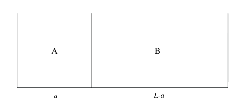
Figure 1: Casimir piston

It is fundamental and significant to study the Casimir force on the piston at finite temperature in the Randall-Sundrum models. Now we choose a piston device depicted in Fig.1. One plate, called a piston, is inserted into a two-parallel-plate system and is parallel to the plates to divide the system into two parts labelled by A and B respectively. In Part A the distance between the left plate and the piston is $a$, the remains of the separation of two original plates is certainly $L-a$, which means that $L$ denotes the whole plates separation. The total vacuum energy density of the massless scalar fields obeying Dirichlet boundary conditions within the region involving a piston shown in Fig.1 can be written as the sun of three terms,

$$\varepsilon=\varepsilon^{A}(a,T)+\varepsilon^{B}(L-a,T)+\varepsilon^{out}(T)$$ (1)

where $\varepsilon^{A}(a,T)$ and $\varepsilon^{B}(L-a,T)$ mean the energy density of Part A and B respectively, and the two terms depend on the temperature and their own size in these two parts. The term $\varepsilon^{out}(T)$ represents the vacuum energy density outside the system under thermal influence and is independent of characteristics inside the system. Having regularized the total vacuum energy density, we obtain the Casimir energy density,

$$\varepsilon_{C}=\varepsilon_{R}^{A}(a,T)+\varepsilon_{R}^{B}(L-a,T)+\varepsilon_{R}^{out}(T)$$ (2)

where $\varepsilon_{R}^{A}(a,T)$, $\varepsilon_{R}^{B}(L-a,T)$ and $\varepsilon_{R}^{out}(T)$ denote the finite parts of terms $\varepsilon^{A}(a,T)$, $\varepsilon^{B}(L-a,T)$ and $\varepsilon^{out}(T)$ in Eq. (1) respectively. It should be pointed out that $\varepsilon^{out}(T)$ is not a function of the position of the piston although it depends on the environment temperature. Further the Casimir force per unit area on the piston is given with the help of derivative of the Casimir energy density with respect to the plates distance like $f^{\prime}_{C}=-\frac{\partial\varepsilon_{C}}{\partial a}$ and can be written as,

$$f^{\prime}_{C}=-\frac{\partial}{\partial a}[\varepsilon_{R}^{A}(a,T)+\varepsilon_{R}^{B}(L-a,T)]$$ (3)

showing that the contribution of vacuum energy from the exterior region does not modify the Casimir force on the piston. According to the previous studies, we should point out that the piston analysis is a correct way to perform the parallel-plate calculation because we can not neglect the contribution to the vacuum energy from the area outside the confined region. Further we wonder how the thermal influence modifies the Casimir effect for parallel plates in the models. This problem, to our knowledge, has not been examined. The main purpose of this paper is to research on the Casimir force between two parallel plates when the environment temperature does not vanish in the Randall-Sundrum models. We obtain the Casimir force on a piston in the system consisting of three parallel plates with nonzero temperature by means of the zeta-function regularization in the RSI and RSII models respectively. We also compute the Casimir force in the limit that one outer plate is moved to the extremely distant place. We discuss the dependence of the reduced force on the temperature and compare our results with those with vanishing temperature and the measurements. Our discussions and conclusions are listed in the end.

II.    The Casimir effect for a piston at finite temperature in the RSI models

Here we discuss a massless scalar field living in the bulk at nonzero temperature in the RS models. Within the frame the spacetime metric is chosen as,

$$ds^{2}=e^{-2k|y|}g_{\mu\nu}dx^{\mu}dx^{\nu}-dy^{2}$$ (4)

where $k$ is assumed to be of the order of the Planck scale which governs the degree of curvature of the $AdS_{5}$ with constant negative curvature. That the extra dimension is compactified on an orbifold gives rise to the generation of the absolute value of $y$ in the metric. The imaginary time formalism can be used to describe the scalar fields in the thermal equilibrium [27, 51-54]. In the five-dimensional RS models we introduce a partition function for a system,

$$Z=N\int_{periodic}D\Phi\exp[\int_{0}^{\beta}d\tau\int d^{3}xdy\mathcal{L}(\Phi,\partial_{E}\Phi)]$$ (5)

where $\mathcal{L}$ is the Lagrangian density for the system under consideration, $N$ a constant and ”periodic” means $\Phi(0,x^{\mu},y)=\Phi(\beta,x^{\mu},y)$. Here $\beta=\frac{1}{T}$ is the inverse of the temperature. In the five-dimensional spacetime with the background metric denoted in Eq. (4), the equation of motion for a massless bulk scalar field $\Phi$ is,

$$g^{\mu\nu}\partial_{\mu}\partial_{\nu}\Phi-e^{2ky}\partial_{y}(e^{-4ky}\partial_{y}\Phi)=0$$ (6)

where $g^{\mu\nu}$ is the usual four-dimensional flat metric with signature $-2$. The field confining between the two parallel plates satisfies the Dirichlet boundary conditions $\Phi(x^{\mu},y)|_{\partial\Omega}=0$, $\partial\Omega$ positions of the plates in coordinates $x^{\mu}$. Following Ref. [50], we can choose the $y$-dependent part of the field $\Phi(x^{\mu},y)$ as $\chi^{(N)}(y)$ in virtue of separation of variables.

The general expression for the nonzero modes can be obtained in terms of the Bessel functions of the first and second kind as,

$$\chi^{(N\neq 0)}(y)=e^{2ky}(a_{1}J_{2}(\frac{m_{N}e^{ky}}{k})+a_{2}Y_{2}(\frac{m_{N}e^{ky}}{k}))$$ (7)

where $a_{1}$ and $a_{2}$ are the arbitrary constants. The effective mass term for the scalar field $m_{N}$ can be obtained by means of integrating out the fifth dimension $y$. In the case of RSI model, the hidden and visible 3-branes are located at $y=0$ and $y=\pi R$ respectively. Here we choose $L_{0}=\pi R$. According to the modified Neumann boundary conditions $\frac{\partial\chi^{(N)}}{\partial y}|_{y=0}=\frac{\partial\chi^{(N)}}{\partial y}|_{y=\pi R}=0$, a general reduced equation reads,

$$m=m_{N}\approx\kappa(N+\frac{1}{4})$$ (8)

where

$$\kappa=\pi ke^{-\pi kR}$$ (9)

here we assume $N\gg 1$ or equivalently $\pi kR\gg 1$ throughout our work.

The modes of the vacuum for parallel plates under the Dirichlet and modified Neumann boundary conditions for plate positions and brane locations respectively as mentioned above in RSI at finite temperature can be expressed as,

$$\omega_{nNl}=\sqrt{p^{2}+(\frac{n\pi}{D})^{2}+m_{N}^{2}+(\frac{2\pi l}{\beta})^{2}}$$ (10)

where

$$p^{2}=p_{1}^{2}+p_{2}^{2}$$ (11)

where $p_{1}$ and $p_{2}$ are the wave vectors in the directions of the unbound space coordinates parallel to the plates surface and $d$ is the distance of the plates. Here $n$ and $N$ represent positive integers and $l$ stands for an integer. The generalized zeta function reads,

$$\zeta_{I}(s;-\partial_{E})=Tr(-\partial_{E})^{-s}\hskip 170.71652pt$$

$$=\int d^{2}k\sum_{n=1}^{\infty}\sum_{N=1}^{\infty}\sum_{l=-\infty}^{\infty}[k^{2}+\frac{n^{2}\pi^{2}}{D^{2}}+\kappa^{2}(N+\frac{1}{4})^{2}+(\frac{2l\pi}{\beta})^{2}]^{-s}$$ (12)

where $\partial_{E}=\frac{\partial^{2}}{\partial\tau^{2}}+\nabla^{2}$ with $\tau=it$. Furthermore, Eq.(12) can also be expressed in terms of the zeta functions of Epstein-Hurwitz type,

$$\zeta_{I}(s;-\partial_{E})\hskip 298.75394pt$$

$$=\frac{2\pi\Gamma(s-1)}{\Gamma(s)}E_{3}(s-1;\frac{\pi^{2}}{D^{2}},\kappa^{2},\frac{4\pi^{2}}{\beta^{2}};0,\frac{1}{4},0)\hskip 156.49014pt$$

$$-\frac{2\pi\Gamma(s-1)}{\Gamma(s)}E_{2}^{\frac{\kappa^{2}}{16}}(s-1;\frac{\pi^{2}}{D^{2}},\frac{4\pi^{2}}{\beta^{2}};0,0)-\frac{\pi\Gamma(s-1)}{\Gamma(s)}E_{2}(s-1;\frac{\pi^{2}}{D^{2}},\kappa^{2};0,\frac{1}{4})$$

$$+\frac{\pi\Gamma(s-1)}{\Gamma(s)}E_{1}^{\frac{\kappa^{2}}{16}}(s-1;\frac{\pi^{2}}{D^{2}};0)-\frac{2\pi\Gamma(s-1)}{\Gamma(s)}E_{2}(s-1;\kappa^{2},\frac{4\pi^{2}}{\beta^{2}};\frac{1}{4},0)\hskip 28.45274pt$$

$$+\frac{2\pi\Gamma(s-1)}{\Gamma(s)}E_{1}^{\frac{\kappa^{2}}{16}}(s-1;\frac{4\pi^{2}}{\beta^{2}};0)+\frac{\pi\Gamma(s-1)}{\Gamma(s)}\kappa^{2-2s}\zeta_{H}(s-1,\frac{1}{4})\hskip 42.67912pt$$ (13)

where the zeta functions of Epstein-Hurwitz type are defined as,

$$E_{p}^{b_{1}b_{2}\cdot\cdot\cdot b_{p}}(s;a_{1},a_{2},\cdot\cdot\cdot,a_{p};c_{1},c_{2},\cdot\cdot\cdot,c_{p})=\sum_{\{n_{j}\}=0}^{\infty}\{\sum_{j=1}^{p}[a_{j}(n_{j}+c_{j})^{2}+b_{j}]^{-s}\}$$ (14)

$$E_{p}(s;a_{1},a_{2},\cdot\cdot\cdot,a_{p};c_{1},c_{2},\cdot\cdot\cdot,c_{p})=\sum_{\{n_{j}\}=0}^{\infty}(\sum_{j=1}^{p}a_{j}(n_{j}+c_{j})^{2})^{-s}$$ (15)

and $\zeta_{H}(s,q)=\sum_{n=0}^{\infty}(n+q)^{-s}$ is the Hurwitz zeta function. The energy density of the two-parallel-plate system with thermal corrections is,

$$\varepsilon_{I}(D,T)=-\frac{1}{2}\frac{\partial}{\partial\beta}(\frac{\partial\zeta_{I}(s;-\partial_{E})}{\partial s}|_{s=0})$$ (16)

We regularize the expression of vacuum energy density of the system containing parallel plates to obtain its finite part at nonzero temperature in RSI model as follows,

$$\varepsilon_{IR}(D,T)\hskip 369.88582pt$$

$$=-\frac{\Gamma(4)}{64\pi^{\frac{5}{2}}\Gamma(\frac{5}{2})}\kappa^{3}\sum_{n=1}^{\infty}\frac{\cos n\pi}{(2n)^{4}}-\frac{\pi^{\frac{3}{2}}}{512\Gamma(\frac{5}{2})}\kappa^{3}\hskip 213.39566pt$$

$$-\frac{\kappa^{2}}{2D}\sum_{n_{1}=1}^{\infty}\sum_{n_{2}=0}^{\infty}n_{1}^{-2}(n_{2}+\frac{1}{4})^{2}K_{2}(2n_{1}\kappa D(n_{2}+\frac{1}{4}))+\frac{\pi}{32}\frac{\kappa^{2}}{D}\sum_{n=1}^{\infty}n^{-2}K_{2}(\frac{\kappa D}{2\sqrt{\pi}}n)\hskip 42.67912pt$$

$$+2^{\frac{1}{2}}\pi^{\frac{1}{2}}\beta^{-\frac{3}{2}}\sum_{n_{1}=1}^{\infty}\sum_{n_{2}=0}^{\infty}\sum_{n_{3}=0}^{\infty}n_{1}^{-\frac{3}{2}}[\frac{n_{2}^{2}\pi^{2}}{D^{2}}+\kappa^{2}(n_{3}+\frac{1}{4})^{2}]^{\frac{3}{4}}K_{\frac{3}{2}}[n_{1}\beta\sqrt{\frac{\pi^{2}n_{2}^{2}}{D^{2}}+\kappa^{2}(n_{3}+\frac{1}{4})^{2}}]$$

$$-2^{\frac{1}{2}}\pi^{2}\beta^{-\frac{3}{2}}\sum_{n_{1},n_{2}=1}^{\infty}(\frac{\frac{\pi^{2}n_{1}^{2}}{D^{2}}+\frac{\kappa^{2}}{16}}{\pi^{2}n_{1}^{2}})^{\frac{3}{4}}K_{\frac{3}{2}}(n_{1}\beta\sqrt{\frac{\pi^{2}n_{2}^{2}}{D^{2}}+\frac{\kappa^{2}}{16}})\hskip 128.0374pt$$

$$+2^{\frac{1}{2}}\pi^{\frac{1}{2}}\beta^{-\frac{1}{2}}\sum_{n_{1}=1}^{\infty}\sum_{n_{2},n_{3}=0}^{\infty}n_{1}^{-\frac{1}{2}}[\frac{\pi^{2}n_{2}^{2}}{D^{2}}+\kappa^{2}(n_{3}+\frac{1}{4})^{2}]^{\frac{5}{4}}[K_{\frac{1}{2}}(n_{1}\beta\sqrt{\frac{\pi^{2}n_{2}^{2}}{D^{2}}+\kappa^{2}(n_{3}+\frac{1}{4})^{2}})$$

$$+K_{\frac{5}{2}}(n_{1}\beta\sqrt{\frac{\pi^{2}n_{2}^{2}}{D^{2}}+\kappa^{2}(n_{3}+\frac{1}{4})^{2}})]\hskip 170.71652pt$$

$$-2^{\frac{1}{2}}\pi^{\frac{1}{2}}\beta^{-\frac{1}{2}}\sum_{n_{1},n_{2}=1}^{\infty}n_{1}^{-\frac{1}{2}}(\frac{\pi^{2}n_{2}^{2}}{D^{2}}+\frac{\kappa^{2}}{16})^{\frac{5}{4}}[K_{\frac{1}{2}}(n_{1}\beta\sqrt{\frac{\pi^{2}n_{2}^{2}}{D^{2}}+\frac{\kappa^{2}}{16}})\hskip 99.58464pt$$

$$+K_{\frac{5}{2}}(n_{1}\beta\sqrt{\frac{\pi^{2}n_{2}^{2}}{D^{2}}+\frac{\kappa^{2}}{16}})]\hskip 199.16928pt$$

$$-8\pi^{-\frac{1}{2}}\Gamma(\frac{3}{2})\zeta(3)\beta^{-3}\sum_{n=1}^{\infty}\frac{\sin\frac{n\pi}{2}}{n}-12\pi\beta^{-4}\Gamma(2)\zeta(4)\hskip 142.26378pt$$ (17)

where $K_{\nu}(z)$ is the modified Bessel function of the second kind. We replace the variable $D$ in Eq. (17) with $a$ and $L-a$ to obtain the Casimir energy densities of Part A and Part B like,

$$\varepsilon_{IR}^{A}(a,T)=\varepsilon_{IR}(a,T)\hskip 42.67912pt$$

$$\varepsilon_{IR}^{B}(L-a,T)=\varepsilon_{IR}(L-a,T)$$ (18)

We obtain the Casimir force per unit area on the piston at finite temperature in the cosmological background like RSI model as follows,

$$f^{\prime}_{IC}=-\frac{\partial}{\partial a}[\varepsilon^{A}_{IR}(a,T)+\varepsilon^{B}_{IR}(L-a,T)]\hskip 184.9429pt$$

$$=-\frac{\kappa^{2}}{2a^{2}}\sum_{n_{1}=1}^{\infty}\sum_{n_{2}=0}^{\infty}n_{1}^{-2}(n_{2}+\frac{1}{4})^{2}K_{2}[2n_{1}\kappa a(n_{2}+\frac{1}{4})]\hskip 142.26378pt$$

$$-\frac{\kappa^{3}}{2a}\sum_{n_{1}=1}^{\infty}\sum_{n_{2}=0}^{\infty}n_{1}^{-1}(n_{2}+\frac{1}{4})^{3}[K_{1}(2n_{1}\kappa a(n_{2}+\frac{1}{4})+K_{3}(2n_{1}\kappa a(n_{2}+\frac{1}{4})))]\hskip 28.45274pt$$

$$+\frac{1}{32}\frac{\kappa^{3}}{a}\sum_{n=1}^{\infty}n^{-2}K_{2}(\frac{\kappa a}{2\sqrt{\pi}}n)+\frac{\pi^{\frac{1}{2}}}{128}\frac{\kappa^{3}}{a}\sum_{n=1}^{\infty}n^{-1}[K_{1}(\frac{\kappa a}{2\sqrt{\pi}}n)+K_{3}(\frac{\kappa a}{2\sqrt{\pi}}n)]\hskip 28.45274pt$$

$$+\frac{3\sqrt{2}\pi^{\frac{5}{2}}}{2}\frac{1}{a^{\frac{5}{2}}\beta^{\frac{3}{2}}}\sum_{n_{1}=1}^{\infty}\sum_{n_{2},n_{3}=0}^{\infty}n_{1}^{-\frac{3}{2}}n_{2}^{2}[\pi^{2}n_{2}^{2}+\kappa^{2}a^{2}(n_{3}+\frac{1}{4})^{2}]^{-\frac{1}{4}}\hskip 71.13188pt$$

$$\times K_{\frac{3}{2}}[n_{1}\frac{\beta}{a}\sqrt{\pi^{2}n_{2}^{2}+\kappa^{2}a^{2}(n_{3}+\frac{1}{4})^{2}}]\hskip 142.26378pt$$

$$+2\sqrt{2}\pi^{\frac{5}{2}}\frac{1}{a^{\frac{7}{2}}\beta^{\frac{1}{2}}}\sum_{n_{1}=1}^{\infty}\sum_{n_{2},n_{3}=0}^{\infty}n_{1}^{-\frac{1}{2}}n_{2}^{2}[\pi^{2}n_{2}^{2}+\kappa^{2}a^{2}(n_{3}+\frac{1}{4})^{2}]^{\frac{1}{4}}\hskip 85.35826pt$$

$$\times(K_{\frac{1}{2}}[n_{1}\frac{\beta}{a}\sqrt{\pi^{2}n_{2}^{2}+\kappa^{2}a^{2}(n_{3}+\frac{1}{4})^{2}}]+K_{\frac{5}{2}}[n_{1}\frac{\beta}{a}\sqrt{\pi^{2}n_{2}^{2}+\kappa^{2}a^{2}(n_{3}+\frac{1}{4})^{2}}])$$

$$-\frac{3\sqrt{2}\pi^{\frac{5}{2}}}{2}\frac{1}{a^{\frac{5}{2}}\beta^{\frac{3}{2}}}\sum_{n_{1},n_{2}=1}^{\infty}n_{1}^{-\frac{3}{2}}n_{2}^{2}(\pi^{2}n_{2}^{2}+\frac{\kappa^{2}a^{2}}{16})^{-\frac{1}{4}}K_{\frac{3}{2}}(n_{1}\frac{\beta}{a}\sqrt{\pi^{2}n_{2}^{2}+\frac{\kappa^{2}a^{2}}{16}})\hskip 28.45274pt$$

$$-2\sqrt{2}\pi^{\frac{5}{2}}\frac{1}{a^{\frac{7}{2}}\beta^{\frac{1}{2}}}\sum_{n_{1},n_{2}=1}^{\infty}n_{1}^{-\frac{1}{2}}n_{2}^{2}(\pi^{2}n_{2}^{2}+\frac{\kappa^{2}a^{2}}{16})^{\frac{1}{4}}\hskip 142.26378pt$$

$$\times[K_{\frac{1}{2}}(n_{1}\frac{\beta}{a}\sqrt{\pi^{2}n_{2}^{2}+\frac{\kappa^{2}a^{2}}{16}})+K_{\frac{5}{2}}(n_{1}\frac{\beta}{a}\sqrt{\pi^{2}n_{2}^{2}+\frac{\kappa^{2}a^{2}}{16}})]\hskip 56.9055pt$$

$$-\frac{\sqrt{2}\pi^{\frac{5}{2}}}{2}\frac{\beta^{\frac{1}{2}}}{\kappa^{\frac{1}{2}}a^{5}}\sum_{n_{1}=1}^{\infty}\sum_{n_{2},n_{3}=0}^{\infty}n_{1}^{\frac{1}{2}}n_{2}^{2}[\pi^{2}n_{2}^{2}+\kappa^{2}a^{2}(n_{3}+\frac{1}{4})^{2}]^{\frac{3}{4}}\hskip 99.58464pt$$

$$\times[K_{-\frac{1}{2}}(n_{1}\frac{\beta}{a}\sqrt{\pi^{2}n_{2}^{2}+\kappa^{2}a^{2}(n_{3}+\frac{1}{4})^{2}})+2K_{\frac{3}{2}}(n_{1}\frac{\beta}{a}\sqrt{\pi^{2}n_{2}^{2}+\kappa^{2}a^{2}(n_{3}+\frac{1}{4})^{2}})$$

$$+K_{\frac{7}{2}}(n_{1}\frac{\beta}{a}\sqrt{\pi^{2}n_{2}^{2}+\kappa^{2}a^{2}(n_{3}+\frac{1}{4})^{2}})]\hskip 113.81102pt$$

$$+\frac{\sqrt{2}\pi^{\frac{5}{2}}}{2}\frac{\beta^{\frac{1}{2}}}{\kappa^{\frac{1}{2}}a^{5}}\sum_{n_{1},n_{2}=1}^{\infty}n_{1}^{\frac{1}{2}}n_{2}^{2}(\pi^{2}n_{2}^{2}+\frac{\kappa^{2}a^{2}}{16})^{\frac{3}{4}}\hskip 170.71652pt$$

$$\times[K_{-\frac{1}{2}}(n_{1}\frac{\beta}{a}\sqrt{\pi^{2}n_{2}^{2}+\frac{\kappa^{2}a^{2}}{16}})+2K_{\frac{3}{2}}(n_{1}\frac{\beta}{a}\sqrt{\pi^{2}n_{2}^{2}+\frac{\kappa^{2}a^{2}}{16}})\hskip 56.9055pt$$

$$+K_{\frac{7}{2}}(n_{1}\frac{\beta}{a}\sqrt{\pi^{2}n_{2}^{2}+\frac{\kappa^{2}a^{2}}{16}})]\hskip 170.71652pt$$

$$+\frac{\kappa^{2}}{2(L-a)^{2}}\sum_{n_{1}=1}^{\infty}\sum_{n_{2}=0}^{\infty}n_{1}^{-2}(n_{2}+\frac{1}{4})^{2}K_{2}[2n_{1}\kappa(L-a)(n_{2}+\frac{1}{4})]\hskip 85.35826pt$$

$$+\frac{\kappa^{3}}{2(L-a)}\sum_{n_{1}=1}^{\infty}\sum_{n_{2}=0}^{\infty}n_{1}^{-1}(n_{2}+\frac{1}{4})^{3}[K_{1}(2n_{1}\kappa(L-a)(n_{2}+\frac{1}{4})\hskip 85.35826pt$$

$$+K_{3}(2n_{1}\kappa(L-a)(n_{2}+\frac{1}{4})))]\hskip 113.81102pt$$

$$-\frac{1}{32}\frac{\kappa^{3}}{L-a}\sum_{n=1}^{\infty}n^{-2}K_{2}(\frac{\kappa(L-a)}{2\sqrt{\pi}}n)\hskip 199.16928pt$$

$$-\frac{\pi^{\frac{1}{2}}}{128}\frac{\kappa^{3}}{L-a}\sum_{n=1}^{\infty}n^{-1}[K_{1}(\frac{\kappa(L-a)}{2\sqrt{\pi}}n)+K_{3}(\frac{\kappa(L-a)}{2\sqrt{\pi}}n)]\hskip 99.58464pt$$

$$-\frac{3\sqrt{2}\pi^{\frac{5}{2}}}{2}\frac{1}{(L-a)^{\frac{5}{2}}\beta^{\frac{3}{2}}}\sum_{n_{1}=1}^{\infty}\sum_{n_{2},n_{3}=0}^{\infty}n_{1}^{-\frac{3}{2}}n_{2}^{2}[\pi^{2}n_{2}^{2}+\kappa^{2}(L-a)^{2}(n_{3}+\frac{1}{4})^{2}]^{-\frac{1}{4}}\hskip 14.22636pt$$

$$\times K_{\frac{3}{2}}[n_{1}\frac{\beta}{L-a}\sqrt{\pi^{2}n_{2}^{2}+\kappa^{2}(L-a)^{2}(n_{3}+\frac{1}{4})^{2}}]\hskip 85.35826pt$$

$$-2\sqrt{2}\pi^{\frac{5}{2}}\frac{1}{(L-a)^{\frac{7}{2}}\beta^{\frac{1}{2}}}\sum_{n_{1}=1}^{\infty}\sum_{n_{2},n_{3}=0}^{\infty}n_{1}^{-\frac{1}{2}}n_{2}^{2}[\pi^{2}n_{2}^{2}+\kappa^{2}(L-a)^{2}(n_{3}+\frac{1}{4})^{2}]^{\frac{1}{4}}\hskip 28.45274pt$$

$$\times(K_{\frac{1}{2}}[n_{1}\frac{\beta}{L-a}\sqrt{\pi^{2}n_{2}^{2}+\kappa^{2}(L-a)^{2}(n_{3}+\frac{1}{4})^{2}}]\hskip 85.35826pt$$

$$+K_{\frac{5}{2}}[n_{1}\frac{\beta}{L-a}\sqrt{\pi^{2}n_{2}^{2}+\kappa^{2}(L-a)^{2}(n_{3}+\frac{1}{4})^{2}}])\hskip 56.9055pt$$

$$+\frac{3\sqrt{2}\pi^{\frac{5}{2}}}{2}\frac{1}{(L-a)^{\frac{5}{2}}\beta^{\frac{3}{2}}}\sum_{n_{1},n_{2}=1}^{\infty}n_{1}^{-\frac{3}{2}}n_{2}^{2}(\pi^{2}n_{2}^{2}+\frac{\kappa^{2}(L-a)^{2}}{16})^{-\frac{1}{4}}\hskip 85.35826pt$$

$$\times K_{\frac{3}{2}}(n_{1}\frac{\beta}{L-a}\sqrt{\pi^{2}n_{2}^{2}+\frac{\kappa^{2}(L-a)^{2}}{16}})\hskip 113.81102pt$$

$$+2\sqrt{2}\pi^{\frac{5}{2}}\frac{1}{(L-a)^{\frac{7}{2}}\beta^{\frac{1}{2}}}\sum_{n_{1},n_{2}=1}^{\infty}n_{1}^{-\frac{1}{2}}n_{2}^{2}(\pi^{2}n_{2}^{2}+\frac{\kappa^{2}(L-a)^{2}}{16})^{\frac{1}{4}}\hskip 85.35826pt$$

$$\times[K_{\frac{1}{2}}(n_{1}\frac{\beta}{L-a}\sqrt{\pi^{2}n_{2}^{2}+\frac{\kappa^{2}(L-a)^{2}}{16}})\hskip 142.26378pt$$

$$+K_{\frac{5}{2}}(n_{1}\frac{\beta}{L-a}\sqrt{\pi^{2}n_{2}^{2}+\frac{\kappa^{2}(L-a)^{2}}{16}})]\hskip 113.81102pt$$

$$+\frac{\pi^{\frac{5}{2}}}{\sqrt{2}}\frac{\beta^{\frac{1}{2}}}{\kappa^{\frac{1}{2}}(L-a)^{5}}\sum_{n_{1}=1}^{\infty}\sum_{n_{2},n_{3}=0}^{\infty}n_{1}^{\frac{1}{2}}n_{2}^{2}[\pi^{2}n_{2}^{2}+\kappa^{2}(L-a)^{2}(n_{3}+\frac{1}{4})^{2}]^{\frac{3}{4}}\hskip 42.67912pt$$

$$\times[K_{-\frac{1}{2}}(n_{1}\frac{\beta}{L-a}\sqrt{\pi^{2}n_{2}^{2}+\kappa^{2}(L-a)^{2}(n_{3}+\frac{1}{4})^{2}})\hskip 85.35826pt$$

$$+2K_{\frac{3}{2}}(n_{1}\frac{\beta}{L-a}\sqrt{\pi^{2}n_{2}^{2}+\kappa^{2}(L-a)^{2}(n_{3}+\frac{1}{4})^{2}})\hskip 56.9055pt$$

$$+K_{\frac{7}{2}}(n_{1}\frac{\beta}{L-a}\sqrt{\pi^{2}n_{2}^{2}+\kappa^{2}(L-a)^{2}(n_{3}+\frac{1}{4})^{2}})]\hskip 56.9055pt$$

$$-\frac{\pi^{\frac{5}{2}}}{\sqrt{2}}\frac{\beta^{\frac{1}{2}}}{\kappa^{\frac{1}{2}}(L-a)^{5}}\sum_{n_{1},n_{2}=1}^{\infty}n_{1}^{\frac{1}{2}}n_{2}^{2}(\pi^{2}n_{2}^{2}+\frac{\kappa^{2}(L-a)^{2}}{16})^{\frac{3}{4}}\hskip 99.58464pt$$

$$\times[K_{-\frac{1}{2}}(n_{1}\frac{\beta}{L-a}\sqrt{\pi^{2}n_{2}^{2}+\frac{\kappa^{2}(L-a)^{2}}{16}})\hskip 85.35826pt$$

$$+2K_{\frac{3}{2}}(n_{1}\frac{\beta}{L-a}\sqrt{\pi^{2}n_{2}^{2}+\frac{\kappa^{2}(L-a)^{2}}{16}})\hskip 85.35826pt$$

$$+K_{\frac{7}{2}}(n_{1}\frac{\beta}{L-a}\sqrt{\pi^{2}n_{2}^{2}+\frac{\kappa^{2}(L-a)^{2}}{16}})]\hskip 85.35826pt$$ (19)

This expression represents the Casimir pressure on the piston before the right plate of the system depicted in Fig. 1 has been moved to the remote place. Further we take the limit $L\longrightarrow\infty$ which means that the right plate in Part B is moved to a very distant place, then we obtain the following expression for the Casimir force per unit area on the piston within the frame of two-brane Randall-Sundrum issue,

$$f_{IC}=\lim_{L\longrightarrow\infty}f^{\prime}_{IC}\hskip 270.30118pt$$

$$=-\frac{\kappa^{4}}{2\mu^{2}}\sum_{n_{1}=1}^{\infty}\sum_{n_{2}=0}^{\infty}n_{1}^{-2}(n_{2}+\frac{1}{4})^{2}K_{2}[2n_{1}\mu(n_{2}+\frac{1}{4})]\hskip 113.81102pt$$

$$-\frac{\kappa^{4}}{2\mu}\sum_{n_{1}=1}^{\infty}\sum_{n_{2}=0}^{\infty}n_{1}^{-1}(n_{2}+\frac{1}{4})^{3}[K_{1}(2n_{1}\mu(n_{2}+\frac{1}{4})+K_{3}(2n_{1}\mu(n_{2}+\frac{1}{4})))]$$

$$+\frac{\pi}{32}\frac{\kappa^{4}}{\mu^{2}}\sum_{n=1}^{\infty}n^{-2}K_{2}(\frac{\mu}{2\sqrt{\pi}}n)+\frac{\pi^{\frac{1}{2}}}{128}\frac{\kappa^{4}}{\mu}\sum_{n=1}^{\infty}n^{-1}[K_{1}(\frac{\mu}{2\sqrt{\pi}}n)+K_{3}(\frac{\mu}{2\sqrt{\pi}}n)]$$

$$+\frac{3\sqrt{2}\pi^{\frac{5}{2}}}{2}\frac{\kappa^{4}}{\mu^{\frac{5}{2}}\xi^{\frac{3}{2}}}\sum_{n_{1}=1}^{\infty}\sum_{n_{2},n_{3}=0}^{\infty}n_{1}^{-\frac{3}{2}}n_{2}^{2}[\pi^{2}n_{2}^{2}+\mu^{2}(n_{3}+\frac{1}{4})^{2}]^{-\frac{1}{4}}\hskip 56.9055pt$$

$$\times K_{\frac{3}{2}}[n_{1}\frac{\xi}{\mu}\sqrt{\pi^{2}n_{2}^{2}+\mu^{2}(n_{3}+\frac{1}{4})^{2}}]\hskip 85.35826pt$$

$$+2\sqrt{2}\pi^{\frac{5}{2}}\frac{\kappa^{4}}{\mu^{\frac{7}{2}}\xi^{\frac{1}{2}}}\sum_{n_{1}=1}^{\infty}\sum_{n_{2},n_{3}=0}^{\infty}n_{1}^{-\frac{1}{2}}n_{2}^{2}[\pi^{2}n_{2}^{2}+\mu^{2}(n_{3}+\frac{1}{4})^{2}]^{\frac{1}{4}}\hskip 71.13188pt$$

$$\times(K_{\frac{1}{2}}[n_{1}\frac{\xi}{\mu}\sqrt{\pi^{2}n_{2}^{2}+\mu^{2}(n_{3}+\frac{1}{4})^{2}}]+K_{\frac{5}{2}}[n_{1}\frac{\xi}{\mu}\sqrt{\pi^{2}n_{2}^{2}+\mu^{2}(n_{3}+\frac{1}{4})^{2}}])$$

$$-\frac{3\sqrt{2}\pi^{\frac{5}{2}}}{2}\frac{\kappa^{4}}{\mu^{\frac{5}{2}}\xi^{\frac{3}{2}}}\sum_{n_{1},n_{2}=1}^{\infty}n_{1}^{-\frac{3}{2}}n_{2}^{2}(\pi^{2}n_{2}^{2}+\frac{\mu^{2}}{16})^{-\frac{1}{4}}K_{\frac{3}{2}}(n_{1}\frac{\xi}{\mu}\sqrt{\pi^{2}n_{2}^{2}+\frac{\mu^{2}}{16}})\hskip 14.22636pt$$

$$-2\sqrt{2}\pi^{\frac{5}{2}}\frac{\kappa^{4}}{\mu^{\frac{7}{2}}\xi^{\frac{1}{2}}}\sum_{n_{1},n_{2}=1}^{\infty}n_{1}^{-\frac{1}{2}}n_{2}^{2}(\pi^{2}n_{2}^{2}+\frac{\mu^{2}}{16})^{\frac{1}{4}}\hskip 128.0374pt$$

$$\times[K_{\frac{1}{2}}(n_{1}\frac{\xi}{\mu}\sqrt{\pi^{2}n_{2}^{2}+\frac{\mu^{2}}{16}})+K_{\frac{5}{2}}(n_{1}\frac{\xi}{\mu}\sqrt{\pi^{2}n_{2}^{2}+\frac{\mu^{2}}{16}})]\hskip 28.45274pt$$

$$-\frac{\pi^{\frac{5}{2}}}{\sqrt{2}}\frac{\kappa^{4}\xi^{\frac{1}{2}}}{\mu^{5}}\sum_{n_{1}=1}^{\infty}\sum_{n_{2},n_{3}=0}^{\infty}n_{1}^{\frac{1}{2}}n_{2}^{2}[\pi^{2}n_{2}^{2}+\mu^{2}(n_{3}+\frac{1}{4})^{2}]^{\frac{3}{4}}\hskip 85.35826pt$$

$$\times[K_{-\frac{1}{2}}(n_{1}\frac{\xi}{\mu}\sqrt{\pi^{2}n_{2}^{2}+\mu^{2}(n_{3}+\frac{1}{4})^{2}})+2K_{\frac{3}{2}}(n_{1}\frac{\xi}{\mu}\sqrt{\pi^{2}n_{2}^{2}+\mu^{2}(n_{3}+\frac{1}{4})^{2}})$$

$$+K_{\frac{7}{2}}(n_{1}\frac{\xi}{\mu}\sqrt{\pi^{2}n_{2}^{2}+\mu^{2}(n_{3}+\frac{1}{4})^{2}})]\hskip 85.35826pt$$

$$+\frac{\pi^{\frac{5}{2}}}{\sqrt{2}}\frac{\kappa^{4}\xi^{\frac{1}{2}}}{\mu^{5}}\sum_{n_{1},n_{2}=1}^{\infty}n_{1}^{\frac{1}{2}}n_{2}^{2}(\pi^{2}n_{2}^{2}+\frac{\mu^{2}}{16})^{\frac{3}{4}}\hskip 142.26378pt$$

$$\times[K_{-\frac{1}{2}}(n_{1}\frac{\xi}{\mu}\sqrt{\pi^{2}n_{2}^{2}+\frac{\mu^{2}}{16}})+2K_{\frac{3}{2}}(n_{1}\frac{\xi}{\mu}\sqrt{\pi^{2}n_{2}^{2}+\frac{\mu^{2}}{16}})\hskip 28.45274pt$$

$$+K_{\frac{7}{2}}(n_{1}\frac{\xi}{\mu}\sqrt{\pi^{2}n_{2}^{2}+\frac{\mu^{2}}{16}})]\hskip 85.35826pt$$ (20)

while we introduce two dimensionless variables, the scaled temperature and the relation between plates separation and the distance between two 3-branes respectively,

$$\xi=\kappa\beta=\pi k\beta e^{-\pi kR}$$ (21)

$$\mu=\kappa a=\pi kae^{-\pi kR}$$ (22)

The terms with series in Eq.(20) converge very quickly and only the first several summands need to be taken into account for numerical calculation in further discussions. If the temperature approaches zero, the Casimir force will recover to be the results of Ref. [51]. We have to perform the burden and surprisingly difficult calculation on Eq. (20) in order to explore the Casimir force on the piston at finite temperature in the cosmological background governed by the RSI model. It is clear that the force expression depends on the plate-piston distance and temperature. For a definite temperature like $\xi=1$, the numerical evaluations of the Casimir force per unit area on the piston from Eq. (20) lead to the data presented in Fig. 1. We find that the sign of the Casimir force is negative when the dimensionless variable $\mu$ defined in (22) is very tiny. When the distance between the plate and piston is larger enough than the branes separation $R$, meaning the value of $\mu$ is sufficiently large, the nature of the Casimir force turns to be repulsive although the force vanishes as the plates separation approaches to infinity like $\lim_{\mu\longrightarrow\infty}f_{IC}=0$. The curves of the dependence of the Casimir force per unit area for the piston on the plates distance for different temperatures are similar. They possess several general characters such as the attractive Casimir force with very small $\mu$ or the repulsive one with sufficiently large $\mu$ and the asymptotic behaviour $f_{IC}(\mu\longrightarrow\infty,T)=0$. All of the expressions for the Casimir forced with thermal corrections have positive maxima. The dependence of the top values of the curves on the scaled temperature $\xi$ defined in Eq. (21) is shown in Fig. 3. The higher temperature or equivalently lower scaled values leads to larger positive top magnitude, which means that the Casimir force between the plate and piston is an increasing function of temperature. The thermal influence has not cancelled the positive nature of Casimir force but results in the stronger repulsive force. In a word, there also appears the repulsive Casimir force between two parallel plates inevitably under thermal influence in the RSI model, which is excluded by the experimental evidence. It should be emphasized that there appears a term like $\frac{\pi}{32}\frac{\kappa^{2}}{D}\sum_{n=1}^{\infty}n^{-2}K_{2}(\frac{\kappa D}{2\sqrt{\pi}}n)$ in our expression (17) and it is the term that finally leads the Casimir force between two parallel plates in the RSI model to become repulsive when the plates separation is not extremely tiny. We also find that our results involving the term $\frac{\pi}{32}\frac{\kappa^{2}}{D}\sum_{n=1}^{\infty}n^{-2}K_{2}(\frac{\kappa D}{2\sqrt{\pi}}n)$ are subject to $m_{N=0}=0$. The term $\frac{\pi}{32}\frac{\kappa^{2}}{D}\sum_{n=1}^{\infty}n^{-2}K_{2}(\frac{\kappa D}{2\sqrt{\pi}}n)$ will not appear if $m_{N=0}=\frac{\kappa}{4}$ is chosen, then the Casimir energy and Casimir force will be the same as Frank et al’s [50, 53], and $m_{N=0}=\frac{\kappa}{4}$ is not acceptable here. It should be pointed out that the equation is valid asymptotically for $N\gg 1$ although the reduced equation (8) for the effective mass of the scalar bulk field is expressed as an approximation. The error is about $3\%$ when $N=1$ and the error is $0.3\%$ and $0.1\%$ for $N=2$ and $N=3$ respectively, etc., displaying that the error drops very quickly with increasing $N$ [53]. The deviation from the approximation in the case of small $N$ can not change the above conclusion.

III.    The Casimir force for a piston at finite temperature in the RSII models

In this section, we proceed with the same study on the Casimir effect in the RSII model, in which the 3-brane at $y=\pi R$ is at infinity. That the 3-brane is moved to the infinity leads the spectrum of the Kaluza-Klein masses to be continuous and run all $m>0$. The generalized zeta function becomes,

$$\zeta_{II}(s;\partial_{E})=Tr(-\partial_{E})^{-s}\hskip 142.26378pt$$

$$=\sum_{n=1}^{\infty}\sum_{l=-\infty}^{\infty}\int_{0}^{\infty}\frac{dm}{k}\int d^{2}p[p^{2}+(\frac{n\pi}{D})^{2}+m^{2}+(\frac{2l\pi}{\beta})^{2}]^{-s}$$ (23)

here the parameter $k$ is the same as in metric (4) and is determined by the 5D Planck mass and bulk cosmological constant. Similarly after the integration the generalized zeta function for RSII model can be expressed with the help of the Epstein zeta functions as,

$$\zeta_{II}(s;\partial_{E})=\frac{\pi^{\frac{3}{2}}}{k}\frac{\Gamma(s-\frac{3}{2})}{\Gamma(s)}E_{2}(s-\frac{3}{2};\frac{\pi^{2}}{D^{2}},\frac{4\pi^{2}}{\beta^{2}})+\frac{\pi^{\frac{3}{2}}}{2k}\frac{\Gamma(s-\frac{3}{2})}{\Gamma(s)}(\frac{\pi}{D})^{3-2s}\zeta(2s-3)$$ (24)

where

$$E_{p}(s;a_{1},a_{2},\cdot\cdot\cdot,a_{p})=\sum_{\{n_{j}\}=1}^{\infty}(\sum_{j=1}^{p}a_{j}n_{j}^{2})^{-s}$$ (25)

and $\zeta(s)$ is the Riemann zeta function. Similarly the vacuum energy density of device involving two parallel plates at finite temperature in the RSII scenario is,

$$\varepsilon_{II}(D,T)=-\frac{1}{2}\frac{\partial}{\partial\beta}(\frac{\partial\zeta_{II}(s;-\partial_{E})}{\partial s}|_{s=0})$$ (26)

We regularize the expressions to obtain the finite parts of the vacuum energy density for parallel plates in the RSII model when the world temperature does not vanish,

$$\varepsilon_{IIR}(D,T)=-\frac{\sqrt{\pi}}{8}\frac{1}{kD^{4}}\Gamma(\frac{5}{2})\zeta(5)+\frac{2\pi^{3}}{k\beta^{2}D^{2}}\sum_{n_{1},n_{2}=1}^{\infty}(\frac{n_{2}}{n_{1}})^{2}K_{2}(\frac{\pi\beta}{D}n_{1}n_{2})$$

$$+\frac{\pi^{4}}{k\beta D^{3}}\sum_{n_{1},n_{2}=1}^{\infty}\frac{n_{2}^{3}}{n_{1}}[K_{1}(\frac{\pi\beta}{D}n_{1}n_{2})+K_{3}(\frac{\pi\beta}{D}n_{1}n_{2})]\hskip 28.45274pt$$

Now we choose the variable $D$ in Eq. (27) as $a$ and $L-a$ respectively to obtain the Casimir energy densities of Part A and Part B as follows,

$$\varepsilon_{IIR}^{A}(a,T)=\varepsilon_{IIR}(a,T)\hskip 42.67912pt$$

$$\varepsilon_{IIR}^{B}(L-a,T)=\varepsilon_{IIR}(L-a,T)$$ (28)

According to Eq. (3), the Casimir per unit area on the piston belonging to a three-parallel-plate system in the RSII model introduces,

$$f^{\prime}_{IIC}=-\frac{\partial}{\partial a}[\varepsilon_{IIR}^{A}(a,T)+\varepsilon_{IIR}^{B}(L-a,T)]\hskip 156.49014pt$$

$$=-\frac{\sqrt{\pi}}{2ka^{5}}\Gamma(\frac{5}{2})\zeta(5)+\frac{4\pi^{3}}{k\beta^{2}a^{3}}\sum_{n_{1},n_{2}=1}^{\infty}(\frac{n_{2}}{n_{1}})^{2}K_{2}(\frac{\pi\beta}{a}n_{1}n_{2})\hskip 113.81102pt$$

$$+\frac{2\pi^{4}}{k\beta a^{4}}\sum_{n_{1},n_{2}=1}^{\infty}\frac{n_{2}^{3}}{n_{1}}[K_{1}(\frac{\pi\beta}{a}n_{1}n_{2})+K_{3}(\frac{\pi\beta}{a}n_{1}n_{2})]\hskip 128.0374pt$$

$$-\frac{\pi^{5}}{2ka^{5}}\sum_{n_{1},n_{2}=1}^{\infty}[K_{0}(\frac{\pi\beta}{a}n_{1}n_{2})+2K_{2}(\frac{\pi\beta}{a}n_{1}n_{2})+K_{4}(\frac{\pi\beta}{a}n_{1}n_{2})]\hskip 56.9055pt$$

$$+\frac{\sqrt{\pi}}{2k(L-a)^{5}}\Gamma(\frac{5}{2})\zeta(5)-\frac{8\pi^{3}}{k\beta^{2}(L-a)^{3}}\sum_{n_{1},n_{2}=1}^{\infty}(\frac{n_{2}}{n_{1}})^{2}K_{2}(\frac{\pi\beta}{L-a}n_{1}n_{2})\hskip 28.45274pt$$

$$-\frac{2\pi^{4}}{k\beta(L-a)^{4}}\sum_{n_{1},n_{2}=1}^{\infty}\frac{n_{2}^{3}}{n_{1}}[K_{1}(\frac{\pi\beta}{L-a}n_{1}n_{2})+K_{3}(\frac{\pi\beta}{a}n_{1}n_{2})]\hskip 85.35826pt$$

$$+\frac{\pi^{5}}{2k(L-a)^{5}}\sum_{n_{1},n_{2}=1}^{\infty}[K_{0}(\frac{\pi\beta}{L-a}n_{1}n_{2})+2K_{2}(\frac{\pi\beta}{L-a}n_{1}n_{2})+K_{4}(\frac{\pi\beta}{L-a}n_{1}n_{2})]$$ (29)

In order to show the Casimir force between the piston and its closer plate and compare our conclusions with the measurements, we let $L\longrightarrow\infty$ to find,

$$f_{IIC}=-\frac{\sqrt{\pi}}{2ka^{5}}\Gamma(\frac{5}{2})\zeta(5)+\frac{4\pi^{3}}{k\beta^{2}a^{3}}\sum_{n_{1},n_{2}=1}^{\infty}(\frac{n_{2}}{n_{1}})^{2}K_{2}(\frac{\pi\beta}{a}n_{1}n_{2})\hskip 113.81102pt$$

$$+\frac{2\pi^{4}}{k\beta a^{4}}\sum_{n_{1},n_{2}=1}^{\infty}\frac{n_{2}^{3}}{n_{1}}[K_{1}(\frac{\pi\beta}{a}n_{1}n_{2})+K_{3}(\frac{\pi\beta}{a}n_{1}n_{2})]\hskip 113.81102pt$$

$$-\frac{\pi^{5}}{2ka^{5}}\sum_{n_{1},n_{2}=1}^{\infty}[K_{0}(\frac{\pi\beta}{a}n_{1}n_{2})+2K_{2}(\frac{\pi\beta}{a}n_{1}n_{2})+K_{4}(\frac{\pi\beta}{a}n_{1}n_{2})]\hskip 56.9055pt$$ (30)

The dependence of the reduced Casimir force per unit area on the plate-piston separation with some values of temperature is plotted in Fig. 4. If the thermal influence is omitted, the above expression of the reduced Casimir pressure will be recovered to be the findings in Ref. [51], just containing a deviation from the results of the conventional parallel-plate system. As the temperature is high enough, i.e. $\beta\longrightarrow 0$, then

$$f_{IIC}(\beta\longrightarrow 0)=-\frac{16\sqrt{\pi}}{k\beta^{5}}\Gamma(\frac{5}{2})\zeta(5)$$ (31)

It is clear that the magnitude of Casimir force on the piston increases with the fifth power of temperature. It also indicates that the sign of the reduced force keeps negative, which means that the plate and piston still attract each other, while higher temperature certainly gives rise to greater attractive Casimir force instead of causing the reduced force to be repulsive. In the four-dimensional flat spacetime the sign of the Casimir force will change to be positive when the temperature is large enough. Our results about the nature of Casimir force between the piston and the remain plate at finite temperature in the context of RSII model are different from those in the background whose dimensionality is four, which are not disfavoured by the measurements.

IV.    Conclusions

The Casimir force between two parallel plates involving the contribution from exterior vacuum energy with thermal corrections is studied in the presence of one warped extra dimension of the models proposed by Randall and Sundrum. In the two-brane scenario called RSI model we derive the Casimir force at finite temperature for the three-parallel-plate system where the middle plate is called piston. We get the exact form of reduced Casimir force per unit area between one plate and the piston as one outer plate is moved away. In this limiting case we find that the sign of the reduced force depending on the temperature and distance between the plate and the piston will become positive when the plate-piston gap is not extremely tiny although the force will disappear as the piston and plate leave far from each other. The stronger thermal influence brings on greater repulsive Casimir force between the plates. In the case of RSI model at finite temperature a repulsive Casimir force is produced due to warps between the parallel plates and the repulsive force is associated with the plates distance, so the repulsive parts of the Casimir force on the piston can not be cancelled although the repulsive parts will vanish when the two parallel plates move away. The appearance of the repulsive Casimir force between one plate and the piston conflicts with the experimental results. It is obvious that the RSI model cannot be reliable according to our analysis even we consider the thermal influence during our research.

In the case of one brane called RSII model we perform the same study and procedure to find the reduced Casimir force per unit area on the piston. We find that the reduced force with thermal corrections is great when the piston and plate are located very closely each other or vanishes with very large plate-piston distance while the force always keeps attractive, no matter how high the temperature is. It is interesting that stronger thermal influence gives rises to greater attractive Casimir force, instead of changing the force to be repulsive.

Acknowledgement

This work was supported by NSFC No. 10875043 and partly supported by the Shanghai Research Foundation No. 07dz22020.

Figure 2: The Casimir force per unit area in unit of $\kappa^{4}$ between the plate and piston versus the dimensionless variable denoted as $\mu=\kappa a$ when $\xi=1$

Figure 3: The dependence of the top values of the Casimir force per unit area in unit of $\kappa^{4}$ between the plate and piston on the scaled temperature $\xi=\kappa\beta$

Figure 4: The dashed, dot and solid curves of Casimir force per unit area on the piston as functions of plate-piston distance in 5-dimensional RSII model for $\beta=0.01,0.011,0.012$ respectively.

References

• [1] Kaluza T. Sitz. Preuss. Akad. Wiss. Phys. Math., 1921, K1: 966
• [2] Klein O. Z. Phys., 1926, 37: 895
• [3] Rubakov V A, Shaposhnikov M E. Phys. Lett. B, 1983, 125: 136
Rubakov V A, Shaposhnikov M E. Phys. Lett. B, 1983, 125: 139
• [4] Visser M. Phys. Lett. B, 1985, 159: 22
• [5] Antoniadis I. Phys. Lett. B, 1990, 246: 317
• [6] Akama K. Prog. Theor. Phys. 1987, 78: 184. ibid, 1988, 79: 1299. ibid, 1989, 80: 935.
Akama K, Hattori T. Mod. Phys. Lett. A, 2000, 15: 2017
• [7] Randall L, Sundrum R. Phys. Rev. Lett., 1999, 83: 3370
• [8] Randall L, Sundrum R. Phys. Rev. Lett., 1999, 83: 4690
• [9] Arkani-Hamed N, Dimopoulos S, Dvali G. Phys. Lett. B, 1998, 429: 263
• [10] Antoniadis I, Arkani-Hamed N, Dimopoulos S, Dvali G. Phys. Lett. B, 1998, 436: 257
• [11] Casimir H B G. Proc. Nederl. Akad. Wetenschap, 1948, 51: 793
• [12] Ambjorn J, Wolfram S. Ann. Phys. (N. Y.), 1983, 147: 1
Plunien G, Muller B, Greiner W. Phys. Rep., 1986, 134: 87
• [13] Elizalde E, Odintsov S D, Romeo A, Bytsenko A A, Zerbini S. Zeta Regularization Techniques with Applications. Singapore: World Scientific Publishing Co. Pte. Ltd., 1994.
• [14] Elizalde E. Ten Physical Applications of Spectral Zeta Functions. Berlin: Springer-Verlag, 1995.
• [15] Bordag M, Mohideen U, Mostepanenko V M. Phys. Rep., 2001, 353: 1
• [16] Milton K A. The Casimir Effect, physical manifestation of zero-point energy. Singapore: World Scientific Publishing Co. Pte. Ltd., 2001.
• [17] Mostepanenko V M, Trunov N N. The Casimir effect and its applications. Oxford: Oxford University Press, 1997.
• [18] Kirsten K. Spectral function in mathematics and physics. London: Chapman and Hall, 2002
• [19] Li X, Cheng H, Li J, Zhai X. Phys. Rev. D, 1997, 56: 2155
• [20] Brevik I, Milton K, Nojiri S, Odintsov S D. Nucl. Phys. B, 2001, 599: 305
• [21] Lamoreaux S K. Phys. Rev. Lett., 1997, 78: 5
• [22] Mohideen U, Roy A. Phys. Rev. Lett., 1998, 81: 4549
• [23] Bressi G, Carugno G, Onfrio R, Ruoso G. Phys. Rev. Lett., 2002, 88: 041804
• [24] Decca R S, Lepez D, Fischbach E, Kraus D E. Phys. Rev. Lett., 2003, 91: 050402
• [25] Alnes H, Ravndal F, Wehus I K, Olaussen K. quant-ph/0607081
• [26] Alnes H, Ravndal F, Wehus I K, Olaussen K. hep-th/0610081
• [27] Cheng H. Chin. Phys. Lett., 2005, 22: 2190
• [28] Poppenhaeger K, Hossenfelder S, Hofmann S, Bleicher M. Phys. Lett. B, 2004, 582: 1
• [29] Cheng H. Chin. Phys. Lett., 2005, 22: 3032
• [30] Cheng H. Mod. Phys. Lett. A, 2006, 21: 1957
• [31] Cheng H. Phys. Lett. B, 2006, 643: 311
• [32] Cavalcanti R M. Phys. Rev. D, 2004, 69: 065015
• [33] Hertzberg M P, Jaffe R I, Kardar M, Scardicchio A. Phys. Rev. Lett., 2005, 95: 250402
• [34] Edery A. Phys. Rev. D, 2007, 75: 105012
• [35] Edery A, MacDonald I. JHEP, 2007, 0709: 005
• [36] Cheng H. Phys. Lett. B, 2008, 668: 72
• [37] Fulling S A, Kirsten K. Phys. Lett. B, 2008, 671: 179
Kirsten K, Fulling S A. Phys. Rev. D, 2009, 79: 065019
• [38] Fulling S A, Kaplan I, Wilson J H. Phys. Rev. D, 2007, 76: 012118
Milton K A, et.al.. Mod. Phys. Lett. A, 2001, 16: 2281
• [39] Elizalde E. J. Phys. A, 2007, 40: 6647
• [40] Greene B R, Levin J. JHEP, 2007, 0711: 096
• [41] Fabinger M, Horava P. Nucl. Phys. B, 2000, 580: 243
• [42] Saharian A A, Setare M R. Phys. Lett. B, 2003, 552: 119
• [43] Cheng H, Li X. Chin. Phys. Lett., 2001, 18: 1163
• [44] Hadasz L, Lambiase G, Nesterenko V V. Phys. Rev. D, 2000, 62: 025011
• [45] Elizalde E, Nojiri S, Odintsov S D, Ogushi S. Phys. Rev. D, 2003, 67: 063515
• [46] Garriga J, Pomarol A. Phys. Lett. B, 2003, 560: 91
• [47] Pujolas O. Int. J. Theor. Phys., 2001, 40: 2131
• [48] Flachi A, Toms D J. Nucl. Phys. B, 2001, 610: 144
• [49] Goldberger W D, Rothstein I Z. Phys. Lett. B, 2000, 491: 339
• [50] Frank M, Turan I, Ziegler L. Phys. Rev. D, 2007, 76: 015008
• [51] Cheng H. Commun. Theor. Phys., 2010, 53: 1125
• [52] Linares R, Morales-Tecotl H A, Pedraza O. Phys. Rev. D, 2008, 77: 066012
• [53] Frank M, Saad N, Turan I. Phys. Rev. D, 2008, 78: 055014
• [54] Satos F C, Tenorio A, Tort A C. Phys. Rev. D, 1999, 60: 105022
• [55] Cheng H. J. Phys. A, 2002, 35: 2205
• [56] Pinto A C A, et al.. Phys. Rev. D, 2003, 67: 107701
• [57] Cognola G, et al.. Mod. Phys. Lett. A, 2004, 19: 1435
Refer to caption