Quantum Computing with Electron Spins in Quantum Dots

Abstract

Several topics on the implementation of spin qubits in quantum dots are reviewed. We first provide an introduction to the standard model of quantum computing and the basic criteria for its realization. Other alternative formulations such as measurement-based and adiabatic quantum computing are briefly discussed. We then focus on spin qubits in single and double GaAs electron quantum dots and review recent experimental achievements with respect to initialization, coherent manipulation and readout of the spin states. We extensively discuss the problem of decoherence in this system, with particular emphasis on its theoretical treatment and possible ways to overcome it.

1 Introduction

It was in the 1980s, when the idea of exploiting quantum degrees of freedom for information processing was envisioned. The central question at the time was whether and how it was possible to simulate (efficiently) any finite physical system with a man-made machine. Deutsch [1] argued that such a simulation is not possible perfectly within the classical computational framework that had been developed for decades. He suggested, together with other researchers such as Feynman [2, 3], that the universal computing machine should be of quantum nature, i.e., a quantum computer.

Around the same time, developments in two different areas of research and industry took a tremendous influence on the advent of quantum computing. On the one hand, it was experimentally confirmed [4] that Nature indeed does possess some peculiar non-local aspects which were heavily debated since the early days of quantum mechanics [5]. Schrödinger [6] coined the term ‘entanglement’, comprising the apparent possibility for faraway parties to observe highly correlated measurement results as a consequence of the global and instantaneous collapse of the wave function according to the Copenhagen interpretation of quantum mechanics. The existence of entanglement is crucial for many quantum computations. On the other hand, the booming computer industry led to major progress in semiconductor and laser technology, a prerequisite for the possibility to fabricate, address and manipulate single quantum systems, as needed in a quantum computer.

As the emerging fields of quantum information and nanotechnology inspired and motivated each other in various ways, and are still doing so today more than ever, many interesting results have been obtained so far, some of them we are about to review in this work. While the theories of quantum complexity and entanglement are being established (a process which is far from being complete) and fast quantum algorithms for classically difficult problems have been discovered, the control and manipulation of single quantum systems is now experimental reality. There are various systems that may be employed as qubits in a quantum computer, i.e., the basic unit of quantum information. Here, we will focus on the idea of using the spins of electrons confined in quantum dots, a proposal made in 1997 [7]. Most knowledge for realizing qubits in the fashion of the spin-qubit proposal of ref. [7] has so far been obtained for quantum dots formed in a two-dimensional electron gas at the interface of a GaAs/AlGaAs heterostructure. Therefore, this is the main type of quantum dot we will turn our attention to. We would nevertheless like to mention that many other systems are investigated intensively at present, such as carbon nanotubes [8], nanowires [9], molecular magnets [10, 11, 12, 13], quantum dots in graphene [14], and nitrogen-vacancy centers in diamond [15, 16, 17, 18].

The idea behind this work is to review quantum computing starting at its very roots, and ending at the current state of knowledge of one of its many branches, here being the spin-qubit proposal of ref. [7] for electron spins in GaAs quantum dots. We approach the subject in the second section by beginning with classical computing and complexity theory, mainly to see the concepts that inspired the so-called standard model of quantum computing discussed later, and to encounter examples of problems that are assumed to be too involved to ever be solved in reasonable time on a classical computer. We then review a set of requirements that every quantum computing proposal should fulfill in order to be usable on a large scale [19]. After discussing the actual spin-qubit proposal of ref. [7], we end the chapter with some recent alternative models of quantum computing and a section about entanglement measures and their numerical evaluation.

While the second section is quite general, we focus in the third section on spin manipulation in GaAs quantum dots. We discuss the latest experimental achievements and we will see that it recently became possible to define, initialize, manipulate, and read out single electron spin qubits with an already quite remarkable rate of success.

Although anticipated to some extent in the third section, the last section intensively discusses the various mechanisms of decoherence and possible ways to reduce its effects, which is a necessary prerequisite for large-scale quantum computing. In greater detail, we investigate the role of the spin-orbit and the hyperfine interaction. We show how these mechanisms cause relaxation of the electron spin, but also how they can be exploited to perform such beneficial tasks as all-electrical single spin manipulation or full polarization of the quantum dot’s nuclear bath.

2 Quantum computing in a nutshell

2.1 Classical computers and complexity theory

Computers are devices that solve problems in an algorithmic fashion. The Church-Turing hypothesis [20, 21] claims that every function which we would naturally regard as being computable by an algorithm (i.e., a procedure that solves a given problem in finite time) can be computed by the universal Turing machine (i.e., a hypothetical, mathematically formalized, programmable discrete machine). Fortunately, the rather cumbersome notion of a Turing machine turns out to be computationally equivalent to a more human-friendly description of algorithms, namely the circuit representation. The basic unit of information, the bit, is a physical system that can be in exactly one out of two states, usually denoted by $0$ and $1$. Information (or data) is stored in binary form using many bits which are represented as lines in the circuit. The data is processed by consecutively applying logical gates to the bits, depicted symbolically as elements acting between the lines in the circuit, such that the desired algorithm is

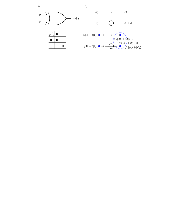
Figure 1: a) Classical xor gate. b) Its quantum analog, i.e., the cnot gate. The truth table of the xor gate is shown in the lower part of a) and simply comes from adding the two input bits modulo 2 (this is the ’$\oplus$’ operation). By replacing $0$ with $|0\rangle$ and $1$ with $|1\rangle$ one obtains the truth table for the target qubit (lower wire) in cnot if the computational basis states are used as input. However, the cnot gate is also the source of entanglement (see also subsect. 2.7) in the standard model of quantum computing, as indicated in the lower part of b) by the fact that, generally, two states cannot be written as a product state $|\psi_{1}\rangle\otimes|\psi_{2}\rangle$ anymore after cnot has been applied.

performed and the solution to the problem is stored in the bits. Examples of such gates include the 1-bit not gate which flips the state of a bit from $0$ to $1$ and vice versa, and the 2-bit xor gate that outputs $1$ if and only if exactly one of the input bits is $1$ (see fig. 1). An important result here is the fact that there exists a set of gates with which one can implement any algorithm in a circuit, provided one can freely distribute and copy information. For classical information, the latter constraint is trivial and the so-called universal set of gates consists in fact of only the nand gate (yielding $0$ if and only if both input bits are 1).

Having set the playground to implement algorithms tackling computational problems, one of the most profound questions one can ask is the following: What is the most efficient algorithm to solve a particular task? It is the field of computational complexity theory [22] that deals with such kind of issues. We will briefly discuss the most important complexity classes, focussing on time rather than space complexity. Imagining that every gate in a circuit requires a finite execution time, one can study the total time required to run an algorithm as a function of the input or problem size, e.g., the number of input bits $n$. A procedure is called efficient (or tractable) if its running time is upper-bounded by some polynomial in $n$. Roughly speaking, the complexity class P consists of all problems known to have efficient algorithms. Sorting or searching lists are examples thereof.

However, there is also a vast amount of problems solved by algorithms that are not efficient (typically exponential in $n$), but once a possible solution has been proposed, it can be efficiently checked for its validity. The class of these types of problems is called NP. An important example thereof is integer factorization: Given an $n$-bit integer, the best known classical algorithm to find its prime factors is exponential in $n$, but given a proposed factorization one can quickly check whether it is correct by doing the required multiplications. The observation that there are problems that can be solved efficiently, and others, for which the best known solution is still worse than polynomial, cumulates in the famous P = NP? question: It is clear that P is a subset of NP, but is this inclusion strict? In other words, have we just not yet discovered efficient algorithms for supposedly ‘hard’ problems, or is there something fundamental within these problems that prevents us from finding such? This puzzling question has not been answered yet with a formal proof, but it is widely assumed that P and NP are not equal.

Another important complexity class is NP-complete, a subset of NP consisting of all problems that are at least as hard as all other problems in NP. This means that every problem in NP can be cast into an instance of a problem in NP-complete in polynomial time. With this transformation being efficient, a polynomial-time solution to any one of the problems in NP-complete would render the whole class NP tractable and it would follow that P = NP. Integer factorization is widely suspected, but not proven, to be both outside of P and NP-complete.

Finally, we remark that there is a complexity class of high practical interest, which we include here merely because it has a quantum analog that we will encounter in subsect. 2.3. Decision problems in the class BPP (for bounded-error probabilistic time) have efficient algorithms that are allowed to make random choices (‘coin flipping’) during the computation and yield the correct answer with probability $p>1/2$, and a wrong solution with probability $1-p$. The choice of $p$ is essentially arbitrary, since the Chernoff bound [23] guarantees that the error probability in a majority vote drops exponentially with the number of repetitive executions of the algorithm. Typically, however, one finds $p=2/3$ or $p=3/4$ in the literature.

2.2 The standard model of quantum computing

In a seminal work by Deutsch [1], he proposes to strengthen the Church-Turing hypothesis into a “manifestly physical and unambiguous” form. His Church-Turing principle reads: “Every finitely realizable physical system can be perfectly simulated by a universal model computing machine operating by finite means”, arguing that “it would surely be hard to regard a function ‘naturally’ as computable if it could not be computed in Nature, and conversely”. It is further shown that the universal Turing machine does not fulfill this principle, while the ‘universal quantum computer’, proposed in the same work, is compatible with the principle. A maybe less theoretic reasoning for studying computing machines operating in the quantum regime is the mere fact that classical computers are governed by Newtonian mechanics, being valid only in a limiting case of the underlying quantum theory [19]. Quantum computers must therefore have at least the same, if not a greater, computational power than classical computers.

Historically understandable, the now so-called standard model of quantum computing [19, 24] follows closely the circuit model discussed earlier (for alternative proposals of quantum computing, see subsect. 2.6). The basic unit of information is the qubit, being a two-level quantum system with basis states usually denoted by $|0\rangle$ and $|1\rangle$ according to its classical counterpart. Qubits are displayed as lines in the circuit to which quantum gates are applied successively, thereby performing the computation. The final result is obtained as a readout (a measurement) of the qubits in the computer’s final state.

The following features distinguish quantum from classical computing. Firstly, quantum states cannot be copied perfectly (this is the no-cloning theorem [25]). Secondly, the nature of a quantum computer is ultimately an analog one. Quantum gates operate on amplitudes such as $\alpha$ and $\beta$ in the state $|\psi\rangle=\alpha|\phi_{1}\rangle+\beta|\phi_{2}\rangle$. Apart from being properly normalized, amplitudes are arbitrary complex numbers and as such analog. Thirdly, qubits can be in superpositions and may form intricate entangled states. This fact is heavily exploited in existing quantum algorithms and is essentially the key ingredient to the majority of them. These first three points all contribute to the drawback that error correction, a necessity in the presence of imperfect gates and decoherence, is a non-trivial thing to do. Quantum error correction, however, turns out to be possible if the error probability per gate is smaller than some finite value for all gates (see criterion 3 in subsect. 2.4). And lastly, quantum gates must be time-reversal, i.e., unitary operators, in accordance with basic principles of quantum mechanics. Apart from the latter, there are no other constraints imposed on quantum gates.

Analogous to the classical case, and quite remarkably, there exist finite sets of gates which can be used to approximate any unitary evolution (i.e., the computation) of the quantum machine to arbitrary precision [26]. An example thereof is the universal set [24] consisting of the two single-qubit gates $H=\frac{1}{\sqrt{2}}\left(\begin{array}[]{cc}1&1\\ 1&-1\\ \end{array}\right)$ and $T=\left(\begin{array}[]{cc}1&0\\ 0&e^{i\pi/4}\\ \end{array}\right)$, and the two-qubit cnot gate which performs the operation $|x\rangle|y\rangle\rightarrow|x\rangle|(x+y)\,\mathop{\mathrm{missing}}{mod}2\rangle$, $x,y\in\{0,1\}$. The gates are represented as usual in the standard computational basis, i.e., $|0\rangle=(1,0)^{T}$ and $|1\rangle=(0,1)^{T}$. The $H$- and $T$- gates are used to approximate arbitrary single-qubit rotations $e^{i\alpha}e^{-i\theta\mathbf{n}\cdot\boldsymbol{\sigma}/2}$, where $\mathbf{n}$ is a real unit vector and $\boldsymbol{\sigma}$ is the vector of Pauli matrices. If arbitrary rotations are available on their own, one can together with the cnot gate implement any unitary evolution exactly.

2.3 Quantum algorithms and quantum complexity

Having the new quantum machine at hand, what is its computational power, and how does it perform compared with classical computers? Such questions have given birth to the new field of quantum complexity theory [27, 28], resulting in a plethora of new quantum complexity classes along with the goal of understanding their relations both between each other, and to classical complexity classes. This is an active field of research and the goal mentioned before is far from being reached. Instead of going into the details of the theory, which would be out of the scope of this work, we sketch an overview of the subject using the most prominent examples.

One of the first algorithms demonstrating that quantum computers may be able to drastically outperform classical computers is the Deutsch-Jozsa algorithm [29, 30]. Let $f$ be a function from $n$ bits to one bit that can either be constant or balanced, the latter meaning that there are exactly $2^{n-1}$ unknown input strings yielding the output $0$. The function is supposed to be implemented in an oracle, i.e., a black box without any further internal specification. The Deutsch-Jozsa algorithm can determine the function’s type (i.e., constant or balanced) with probability $1$ by querying the oracle just once. A deterministic classical algorithm requires $2^{n-1}+1$ queries in the worst case, as one may coincidentally pick all the $2^{n-1}$ input strings that yield the same output. The Deutsch-Jozsa algorithm obtains its power from bringing a register of $n$ qubits into an equally weighted superposition of all possible bit strings using a Hadamard transform which is a special case of a so-called quantum Fourier transform [24]. Using this state as the input for the oracle, the function can be evaluated simultaneously on all strings in the superposition with just one query. This functionality in quantum computing is referred to as quantum parallelism. Without going into further details, the Deutsch-Jozsa algorithm manages to output the correct result with certainty using these techniques. However, one has to be cautious not to get the impression that one can calculate and obtain all function values of an arbitrary function with just one query of an oracle. In general, one is left with a superposition of results collapsing upon measurement and yielding just one function value. The Deutsch-Jozsa algorithm is cleverly designed to work with certainty for a particular type of problem. These ideas are not straightforwardly adapted to problems involving other kinds of functions. The constant/balanced problem is an example from the class EQP (exact quantum polynomial-time) [27], denoting all problems solved in polynomial time by a quantum algorithm with success probability equal to $1$. EQP is the analog to the classical complexity class P.

On the other hand, the set of problems having tractable algorithms on a quantum computer with error probability smaller than $p=1/3$ is denoted by BQP (bounded-error quantum polynomial-time) [27], its classical counterpart being BPP. It contains more interesting problems whose solutions are of greater relevance than the Deutsch-Jozsa algorithm. Famous examples thereof are Grover’s [31] and Shor’s [32] algorithms. Grover’s algorithm searches an unsorted database in time upper-bound by a function proportional to $\sqrt{N}$ and has a probability of failure scaling as $1/N$, where $N$ is the number of database entries. Although the speed-up with respect to the classical database search which runs in time proportional to $N$ is not exponential, it is still of great benefit especially for large $N$. Grover’s algorithm could be used to speed up brute-force search attempts for finding solutions to computationally hard problems. However, probably the most prominent problem in BQP is integer factorization. Shor [32] has shown that a quantum computer can factor an integer in polynomial time, a task which is supposed to be exponentially hard on a classical computer. These kind of discoveries have resulted in a tremendous increase of interest in quantum computing. For example, Shor’s algorithm can be used to break present-day public-key cryptosystems who rely on the hardness of factorizing integers being a product of two large prime numbers (such as RSA [33]).

A quantum complexity class that has recently called attention is QMA [34, 35] (quantum Merlin-Arthur), which can be seen as a quantum analog of NP. Equivalently to the definition in subsect. 2.1, NP can be characterized in terms of decision problems (having either ‘yes’ or ‘no’ as answer): NP contains all problems for which ‘yes’-instances are supplied with a proof that can be checked in polynomial time by a deterministic verifier. For quantum computers, deterministic verifiers are however not meaningful. QMA is thus defined probabilistically: A decision problem belongs to QMA, if for every instance $x$ there exists an efficient (i.e., polynomial in $x$) description of a quantum circuit $Q_{x}$ (the verifier), such that for every ‘yes’-instance $\tilde{x}$ there exists a proof $|\psi\rangle$ with $p(Q_{\tilde{x}}\;\mathrm{accepts}\;|\psi\rangle)>2/3$, and for every ‘no’-instance $\bar{x}$ $p(Q_{\bar{x}}\;\mathrm{accepts}\;|\chi\rangle)<1/3$ holds for all input states $|\chi\rangle$. Here, $p(Q_{x}\;\mathrm{accepts}\;|\psi\rangle)$ denotes the probability to measure, e.g., $|0\rangle$ (if this is defined to mean ‘accept’) as the output of a quantum computation described by the circuit $Q_{x}$ and started with the initial state $|\psi\rangle$.

An important problem known to be in QMA is $k$-local Hamiltonian which is specified by the following decision problem: Given a Hamiltonian $H$ acting on $n$ qubits with interactions that do not involve more than $k$ particles ($k$-body interactions, where $k$ is a constant independent of $n$) and two real numbers $a$ and $b$, such that $b-a>1/\mathrm{poly}(n)$. Is the ground state energy of $H$ smaller than $a$ (‘yes’), or are all energies larger than $b$ (‘no’)? A ‘yes’ instance can be verified by providing an eigenstate with energy smaller than $a$. Furthermore, one can show that polynomial verifiers can be constructed that accept (reject) ‘yes’ instances (‘no’ instances) with sufficient probability. It is now known that $k$-local Hamiltonian is QMA-complete for $k\geq 2$ [36], meaning the following: Given an instance $x$ of any problem $Q$ in QMA, one can find (in time poly($n$)) an instance of $k$-local Hamiltonian (by constructing a $k$-local $H$ and specifying properly chosen parameters $a$ and $b$), such that, if $x$ is a ‘yes’ instance of $Q$, the ground state energy of $H$ is smaller than $a$, and if $x$ is a ‘no’ instance, the smallest eigenvalue of $H$ is larger than $b$. $k$-local Hamiltonian (for $k\geq 2$) is as hard as any other problem in QMA. This ‘hardness’ suggests that calculating the ground state energy, and possibly other ground state properties, is intractable even on a quantum computer. The study of $k$-local Hamiltonian is also important in the context of adiabatic quantum computing, see subsubsect. 2.6.2.

2.4 General criteria for scalable quantum computing

In this section, we review the five DiVincenzo criteria [19] for the physical implementation of quantum computing. These are the most fundamental requirements any proposal for a quantum computer must fulfill in order to work with an arbitrary number of qubits. Starting from sect. 3, we will examine the experimental and theoretical progress toward realizing these criteria for the spin-qubit proposal of ref. [7] (see the next section).

1. A scalable physical system with well characterized qubits.

We have already defined the notion of a qubit as simply being a two-level quantum system. In this review, we will focus solely on the electron spin in quantum dots. The word ‘scalable’ plays an important role: Even if current fundamental experiments are performed with only few qubits, they must at least in principle be preparable or manufacturable in large numbers, since only in this case interesting and useful quantum computations can be performed.

A qubit must also be ‘well characterized’ in the sense that one has a good theoretical description not only of the qubit itself (in terms of an internal Hamiltonian, accurate knowledge of all physical parameters, etc.), but also of all relevant mechanisms that couple qubits among each other and to the environment. On the one hand, this is necessary to explore the possibilities of manipulating qubits and letting them interact, but also, on the other hand, in order to understand and fight the various forms of decoherence a qubit may suffer from (see sect. 4).

2. The ability to initialize the state of the qubits to a simple fiducial state.

It is clear that every computation needs to be started in an initially known state such as $|000\ldots\rangle$. But this is not the end of the story. Having a fast initialization mechanism at hand is crucial for quantum error correction (see next criterion), typically requiring large amounts of ancillary qubits in known initial states in order to perform its job properly. If a fast zeroing of qubits is not possible, i.e., if the initialization time is long compared to gate operation times, then ref. [19] proposes to equip the quantum computer with “some kind of ‘qubit conveyor belt’, on which qubits in need of initialization are carried away from the region in which active computation is taking place, initialized while on the ‘belt’, then brought back to the active place after the initialization is finished.”

In spin qubits, initialization could be achieved by either forcing the spins to align with a strong externally applied magnetic field, or by performing a measurement on the dot followed by a subsequent rotation of the state depending on the measurement outcome. The first approach is somewhat problematic, since natural thermalization times are always longer than the decoherence time which itself needs to be much longer than gate operation times (see the next criterion). In this case, a ‘conveyor belt’ scheme would be required. The second possibility of measurement and rotation depends on the specific setup examined, but initialization times might in principle be much shorter than natural relaxation times. See subsects. 2.5 and 3.2 for more information and recent experimental achievements.

3. Long relevant decoherence times, much longer than the gate operation time.

Due to the coupling of qubits to their environment in a thermodynamically irreversible way, quantum coherence is lost. In other words, quantum states in contact with the outside world ultimately evolve into fully mixed states. Decoherence is the answer to why the macroscopic world looks classical. In GaAs quantum dots where electron spins are used as qubits, the most important mechanisms of decoherence are the spin-orbit and the hyperfine interaction, see subsect. 3.3 and  sect. 4.

If it were not for quantum error correction, the duration of a quantum computation would eventually be determined by the shortest decoherence time in the setup. This would render longer and more complex computations impossible. By encoding information not directly into single qubits, but rather into ‘logical qubits’ consisting of several single qubits, a certain amount of errors due to decoherence and imperfect gates may be corrected, depending on what kind of code is used. There is however still a limit on how faulty elementary gates are allowed to be: The accuracy threshold theorem [37] states that error correction is possible if the error probability per gate is smaller than a certain threshold. This threshold comes about the fact that encoding, verification, and correction steps require an additional overhead of quantum gates, which introduces new possible sources of errors. Error correction is thus only meaningful if encoding reduces the error probability of an encoded operation compared with its original (‘unencoded’) counterpart, despite the fact that more elementary gates are required. By employing the technique of code concatenation [37], i.e., encoding logical qubits recursively, where using different codes per concatenation level is allowed, the effective error on the top level of concatenation can be made arbitrarily small. The threshold value depends on the error models studied and on the details of the codes considered. Typical values are in the range of $10^{-5}$ to $10^{-3}$ [37, 38], implying that decoherence times must be a thousand to a hundred thousand times longer than gate operation times.

4. A “universal” set of quantum gates.

We have mentioned in subsect. 2.2 that generic quantum computing is possible in the standard model if certain one- and two-qubit gates are available. The single qubit gates may be either implemented directly, or can be approximated to arbitrary precision using a finite set of gates. The only necessary two-qubit gate is the controlled-not gate [26]. If these gates are for some reason not implementable directly (i.e., in the sense that there are no Hamiltonians that can be switched on which perform exactly the desired gate operations), then a set capable of synthesizing them needs to be present. This is, e.g., the case in the spin-qubit proposal of ref. [7], where the only controllable two-qubit interaction is the exchange coupling between neighboring spins. The cnot gate can however be implemented using a series of one-qubit operations and the exchange interaction alone. The details and requirements for this to work are discussed in the next section.

It is worth pointing out that one also needs to be able to execute quantum gates in parallel in order for error correction to work. This does however not pose a major drawback for solid-state systems [39], where usually only two-body nearest-neighbor interactions are realizable. It is also important to note the fact that faulty gates may introduce systematic or random errors in a calculation. This can be viewed as a source of decoherence and can therefore be overcome by means of quantum error correction if the error rate is sufficiently small. The same threshold values as discussed in the previous criterion hold in this case.

5. A qubit-specific measurement capability.

Measuring qubits without disturbing the rest of the quantum computer is required in the verification steps of quantum error correction and, not remarkably, in order to reveal the outcome of a computation. If the measurement procedure does not discard qubits (which could be the case, e.g., for spin-dependent tunneling of electrons out of a quantum dot) it may be used in the initialization step (see 2nd criterion). If it is, additionally, fast enough, it may also be useful for quantum error correction. A measurement is said to have $100\%$ quantum efficiency if it yields, performed on a state $\rho=p|0\rangle\langle 0|+(1-p)|1\rangle\langle 1|+\alpha|0\rangle\langle 1|+\alpha^{\ast}|1\rangle\langle 0|$, the outcome “0” with probability $p$ and “1” with probability $(1-p)$ independent of $\alpha$, the states of neighboring qubits, or any other parameters of the system. Real measurements cannot have perfect quantum efficiency. But this is also not required since one can, e.g., rerun the computation several times.

2.5 The Loss-DiVincenzo proposal

In this section, we review the spin-qubit proposal of ref. [7] for universal scalable quantum computing. Here, the physical system representing a qubit is given by the localized spin state of one electron, and the computational basis states $|0\rangle$ and $|1\rangle$ are identified with the two spin states $|{\uparrow\rangle}$ and $|{\downarrow\rangle}$, respectively. In general, the considerations discussed in ref. [7] are applicable to electrons confined to any structure, such as, e.g., atoms, defects, or molecules. However, the original proposal focuses on electrons localized in electrically gated semiconductor quantum dots. The relevance of such systems has become clearer in recent years, where remarkable progress in the fabrication and control of single and double GaAs quantum dots has been made (see, e.g., ref. [40] for a recent experimental review). We postpone the discussion of experimental achievements with respect to satisfying the DiVincenzo criteria to sect. 3.

Scalability in the proposal of ref. [7] is due to the availability of local gating. Gating operations are realized through the exchange coupling (see below), which can be tuned locally with exponential precision. Since neighboring qubits can be coupled and decoupled individually, it is sufficient to study and understand the physics of single and double quantum dots together with the coupling mechanisms to the environment present in particular systems [41]. Undesired interactions between three, four, and more qubits should then not pose any great concern. This is in contrast with proposals that make use of long-ranged interactions (such as dipolar coupling), where scalability might not be easily achieved.

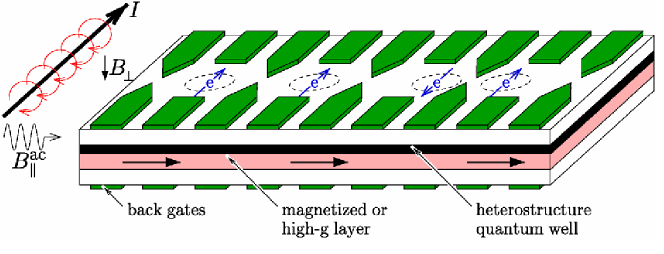
Figure 2: An array of quantum dot qubits realized by laterally confining electrons in a two dimensional electron gas formed at the interface of a heterostructure. The confinement is achieved electrostatically by applying voltages to the metallic top gates. Interaction is generally suppressed (as for the two qubits on the left) but may be turned on to realize two-qubit operations by lowering inter-dot gates (as for the two qubits on the right). Single spin rotations may be achieved by dragging electrons down (by changing back gate voltages) to a region where the Zeeman splitting in the presence of the external static magnetic field $B_{\bot}$ changes due to magnetization or an inhomogeneous $g$-factor present in that layer. A resonant magnetic ac pulse $B_{||}^{\mathrm{a}c}$ can then be used to rotate the spin under consideration, while leaving all other qubits unaffected due to the off-resonant Zeeman splitting (ESR). All-electrical single spin manipulation may be realized in the presence of spin-orbit interaction by applying ac electric pulses directly via the gates (EDSR). See subsect. 3.4 for more details.

Figure 2 displays part of a possible implementation of a quantum computer. Displayed are four qubits represented by the four single electron spins confined vertically in the heterostructure quantum well and laterally by voltages applied to the top gates. Initialization of the quantum computer could be realized at low temperature $T$ by applying an external magnetic field $B$ satisfying $|g\mu_{B}B|\gg k_{B}T$, where $g$ is the $g$-factor, $\mu_{B}$ is Bohr’s magneton, and $k_{B}$ is the Boltzmann constant. After a sufficiently long time, virtually all spins will have equilibrated to their thermodynamic ground state $|0\rangle=|{\uparrow}\rangle$. As discussed in the 2nd criterion of the last section, this method might be too slow for zeroing qubits in a running computation. Other proposed techniques include initialization through spin-injection from a ferromagnet, as has been performed in bulk semiconductors [42, 43], with a spin-polarized current from a spin-filter device [44, 45, 7, 46, 47], or by optical pumping [48, 49, 50, 51]. The latter method has allowed the preparation of spin states with very high fidelity, in one case as high as $99.8\%$ [52].

The proposal of ref. [7] requires single qubit rotations around a fixed axis in order to implement the cnot gate (see below). In the original work [7] this is suggested to be accomplished by varying the Zeeman splitting on each dot individually, which was proposed to be done via a site-selective magnetic field (generated by, e.g., a scanning-probe tip) or by controlled hopping of the electron to a nearby auxiliary ferromagnetic dot. Local control over the Zeeman energy may also be achieved through $g$-factor modulation [53], the inclusion of magnetic layers [54] (see also fig. 2) or by modification of the local Overhauser field due to hyperfine couplings [55]. Arbitrary rotations may be performed via ESR induced by an externally applied oscillating magnetic field (see subsect. 3.4). In this case, however, site-selective tuning of the Zeeman energy is still required in order to bring a specific electron in resonance with the external field, while leaving the other electrons untouched (see also fig. 2). Alternative all-electrical proposals (i.e., without the need for local control over magnetic fields) in the presence of spin-orbit interaction or a static magnetic field gradient have been discussed recently. See subsubsect. 3.4.1 for greater details.

Two-qubit nearest-neighbor interaction is controlled in the proposal of ref. [7] by electrical pulsing of a center gate between the two electrons. If the gate voltage is high, the interaction is ‘off’ since tunneling is suppressed exponentially with the voltage. On the other hand, the coupling can be switched ‘on’ by lowering the central barrier for a certain switching time $\tau_{s}$. In this configuration, the interaction of the two spins may be described in terms of the isotropic Heisenberg Hamiltonian

$$H_{s}(t)=J(t)\mathbf{S}_{L}\cdot\mathbf{S}_{R},$$ (1)

where $J(t)\propto t_{0}^{2}(t)/U$ is the time-dependent exchange coupling that is produced by turning on and off the tunneling matrix element $t_{0}(t)$ via the center gate voltage. $U$ denotes the charging energy of a single dot, and $\mathbf{S}_{L}$ and $\mathbf{S}_{R}$ are the spin-$\frac{1}{2}$ operators for the left and right dot, respectively. Equation (1) is a good description of the double-dot system if the following criteria are satisfied: (i) $\Delta E\gg k_{B}T$, where $T$ is the temperature and $\Delta E$ the level spacing. This means that the temperature cannot provide sufficient energy for transitions to higher-lying orbital states, which can therefore be ignored. (ii) $\tau_{s}\gg\Delta E/\hbar$, requiring the switching time $\tau_{s}$ to be such that the action of the Hamiltonian is ‘adiabatic enough’ to prevent transitions to higher orbital levels. (iii) $U>t_{0}(t)$ for all $t$ in order for the Heisenberg approximation to be accurate. (iv) $\Gamma^{-1}\gg\tau_{s}$, where $\Gamma^{-1}$ is the decoherence time. This is basically a restatement of the 3rd DiVincenzo criterion. For recent experimental results on the decoherence times in lateral GaAs quantum dots, see subsubsect. 3.3.3.

The pulsed Hamiltonian eq. (1) applies a unitary time evolution $U_{s}(t)$ to the state of the double dot given by $U_{s}(t)=\mathcal{T}\exp[-i\int_{0}^{t}H_{s}(t^{\prime})dt^{\prime}/\hbar]=\exp[-(i/\hbar)\int_{0}^{t}J(t^{\prime})dt^{\prime}\mathbf{S}_{L}\cdot\mathbf{S}_{R}]$. If the constant interaction $J(t)=J_{0}$ is switched on for a time $\tau_{s}$ such that $\int_{0}^{\tau_{s}}J(t)dt/\hbar=J_{0}\tau_{s}/\hbar=\pi\mod 2\pi$, then $U_{s}(\tau_{s})$ exchanges the states of the qubits: $U_{s}(\tau_{s})|\mathbf{n},\mathbf{n^{\prime}}\rangle=|\mathbf{n^{\prime}},\mathbf{n}\rangle$. Here, $\mathbf{n}$ and $\mathbf{n^{\prime}}$ denote real unit vectors and $|\mathbf{n},\mathbf{n^{\prime}}\rangle$ is a simultaneous eigenstate of the two operators $\mathbf{S}_{L}\cdot\mathbf{n}$ and $\mathbf{S}_{R}\cdot\mathbf{n^{\prime}}$. This gate is called swap. If the interaction is switched on for the shorter time $\tau_{s}/2$, then $U_{s}(\tau_{s}/2)=U_{s}(\tau_{s})^{1/2}$ performs the so-called ‘square-root of swap’ denoted by $\sqrt{\textsc{swap}}$. This gate together with single-qubit rotations about a fixed (say, the $z$-) axis can be used to synthesize the cnot operation [7]

$$U_{\textsc{cnot}}=e^{i(\pi/2)S_{L}^{z}}e^{-i(\pi/2)S_{R}^{z}}U_{s}(\tau_{s})^{1/2}e^{i\pi S_{L}^{z}}U_{s}(\tau_{s})^{1/2},$$ (2)

or, alternatively, as

$$U_{\textsc{cnot}}=e^{i\pi S_{L}^{z}}U_{s}(\tau_{s})^{-1/2}e^{-i(\pi/2)S_{L}^{z}}U_{s}(\tau_{s})e^{i(\pi/2)S_{L}^{z}}U_{s}(\tau_{s})^{1/2}.$$ (3)

The latter representation has the potential advantage that single qubit rotations involve only one spin, in this case the one in the left dot. Writing the cnot gate as above, it is seen that arbitrary single qubit rotations together with the $\sqrt{\textsc{swap}}$ gate are sufficient for universal quantum computing. See subsect. 3.4 for a recent experimental implementation of the $\sqrt{\textsc{swap}}$ operation. Errors during the execution of a $\sqrt{\textsc{swap}}$ gate due to non-adiabatic transitions to higher orbital states [56, 57], spin-orbit interaction [58, 59, 60], and hyperfine coupling to surrounding nuclear spins [61, 62, 63, 64] have been studied. Furthermore, realistic systems will include some anisotropic spin terms in the exchange interaction which may cause additional errors. Conversely, this fact might be used to perform universal quantum computing with two-spin encoded qubits, in the absence of single-spin rotations [58, 65, 66, 67].

2.6 Alternative approaches to quantum computing

Although the remainder of the review will mostly be concerned with the realization of the spin-qubit proposal of ref. [7] (and related decoherence effects), we would nevertheless like to discuss some of the alternative proposals for quantum computing that have emerged in recent years. Note that by this we are not referring to the many alternative physical implementations of qubits which are also studied extensively in present-day research (see, e.g., ref. [68] for a review focussing mainly on solid state qubits). Rather, we would like to review proposals for quantum computers which fundamentally differ from the standard circuit model. The schemes we will turn our attention to are measurement-based and adiabatic quantum computing. We will not discuss topological quantum computing in greater detail, which performs computation by braiding non-Abelian anyons. These are particular quasi-particle excitations predicted to exist in certain two-dimensional strongly correlated many-body systems such as a two-dimensional electron gas in the fractional quantum Hall regime. Topological quantum computing is supposed to be much less susceptible to gate errors since small deformations of braids do not change their topology. The interested reader is referred to the recent reviews refs. [69, 70]. See ref. [71] for a measurement based implementation of cnot on $\nu=5/2$ Ising-type anyon qubits.

2.6.1 Measurement-based quantum computing

Implementing quantum gates, particularly two-qubit gates, with a precision as required by fault-tolerant error correction is difficult. Instead of performing gate operations on qubits, there are proposals that allow for universal quantum computing by replacing part or all of these gates by measurement. We will mainly focus on a measurement-based implementation of cnot for qubits represented by single or multiple electron spins. Afterwards, we will briefly outline the ideas behind the so-called ‘one-way quantum computer’.

Measurement-based implementation of cnot

When using the polarization state of a photon as a qubit, it is known that universal quantum computing can be achieved using only linear optics and single photon measurements [72]. This holds similarly for all bosons. For electrons (and, similarly, for all fermions), there exists a strong no-go theorem [73, 74] stating that quantum computing with single-electron Hamiltonians and single-spin measurements can efficiently be simulated on a classical computer, thus not exhibiting the observed exponential speed-up of some algorithms over their classical analogs. However, the no-go theorem can be circumvented by exploiting the electron’s charge degree of freedom: It has been shown recently how to build a cnot gate for single- [75] and multi-electron [71] qubits by the ability to perform, apart from the availability of single-electron operations and single-spin readouts, charge measurements. Universal quantum computing is thereby restored. Note that the qubits are still encoded in spin states of electrons. Since spin and charge are commuting observables, charge measurements do not alter the information represented in the spins.

The main idea is to provide parity measurement of two electron spins via charge detection. The cnot gate is then constructed from these parity gates. Imagine we had such a device at hand, i.e., for a state in a space either spanned by $\{|{\uparrow\uparrow}\rangle,|{\downarrow\downarrow}\rangle\}$ (even parity), or by $\{|{\uparrow\downarrow}\rangle,|{\downarrow\uparrow}\rangle\}$ (odd parity), it could determine nondestructively which space the state belongs to by detecting the presence or absence of charge upon a measurement thereof. A rather abstract notion of a parity gate was described in ref. [75]. Further below, we will describe a much more concrete theoretical proposal in the reach of present-day experiments. In the following, however, we will first review the realization of a cnot gate for single-electron qubits as presented in ref. [75]. A generalization of this proposal to multi-electron qubits can be found in ref. [71]. Particularly, a detailed construction of the cnot gate for two-electron qubits encoded in the singlet-triplet basis (see subsect. 3.2) is discussed there.

Let a parity gate work as follows. Two electrons can enter the gate simultaneously, and after the parity was measured via charge detection, the electrons leave the gate with unmodified spin state if the latter was in one of the even or odd parity spaces described above.

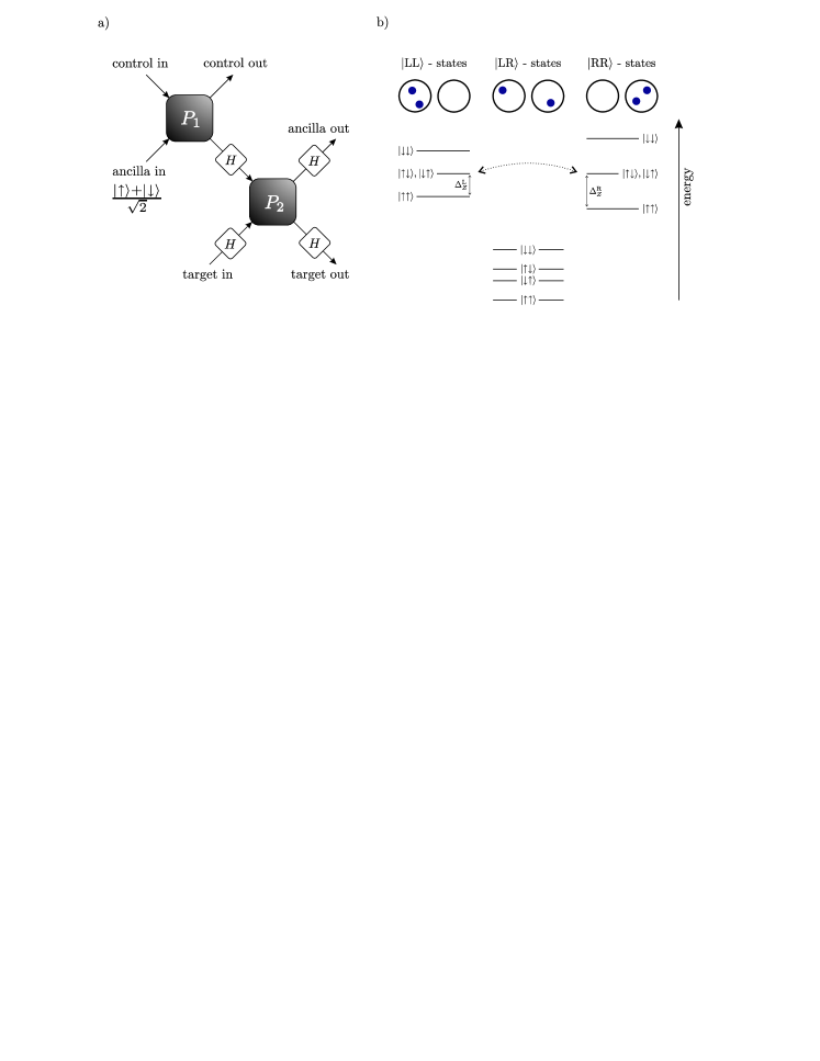
Figure 3: a) Construction of a deterministic cnot gate from two parity gates $P_{1}$ and $P_{2}$. Each parity gate has two input and two output arms and can discriminate whether two incident electrons are in a parallel or antiparallel spin configuration via charge sensing. The gates $H$ symbolize Hadamard transformations. The cnot operation is completed by applying Pauli rotations to the control and target electron depending on the outcomes of the two parity and the ancilla measurements. See main text for a detailed discussion. (Figure adapted from ref. [75].) b) Energy diagram for the double-dot parity gate proposed in ref. [76]. The charge states $|\mathrm{LL}\rangle$, $|\mathrm{LR}\rangle$, and $|\mathrm{RR}\rangle$ are indicated by the electron configuration in the double dot. The energy levels of all possible spin states are shown for each charge configuration. Gate voltages and a magnetic field are applied such that the $|\mathrm{LR}\rangle$ states are lowest in energy, and the antiparallel $|\mathrm{LL}\rangle$ and $|\mathrm{RR}\rangle$ states are on the same energy. This allows for resonant tunneling between the latter two states (indicated by the dotted arrow), while tunneling between parallel states is suppressed due to the Zeeman mismatch $\Delta_{Z}^{\mathrm{R}}>\Delta_{Z}^{\mathrm{L}}$. (Figure adapted from ref. [76].)

Furthermore, let the gate record ‘no charge’ ($p=0$) for two antiparallel spins, and ‘charge’ ($p=1$) for parallel incident spins. Figure 3 a displays the construction of the deterministic cnot gate using two connected parity gates $P_{1}$ and $P_{2}$. Before the input and after the output arms of $P_{2}$, a Hadamard transformation $H$ is applied to each spin, defined as $|{\uparrow}\rangle\rightarrow(|{\uparrow}\rangle+|{\downarrow}\rangle)/\sqrt{2}$, and $|{\downarrow}\rangle\rightarrow(|{\uparrow}\rangle-|{\downarrow}\rangle)/\sqrt{2}$. The control qubit enters the first gate $P_{1}$. Its state decides whether the target qubit, entering the second gate $P_{2}$, is to be flipped according to the definition of the cnot operation. $P_{1}$ is also provided with an ancilla qubit prepared in the state $(|{\uparrow}\rangle+|{\downarrow}\rangle)/\sqrt{2}$ which is then fed back into $P_{2}$. Upon leaving the second gate, the ancilla is measured. Conditioned on this result and the outcomes $p_{1}$ and $p_{2}$ of the two parity measurements in $P_{1}$ and $P_{2}$, respectively, a Pauli matrix has to be applied to control and target qubit in order to complete the cnot operation (see below). We will now see (following the supplementary appendix of ref. [75]) that this setup indeed implements cnot.

We depart from our usual notation for the spin basis and identify $|0\rangle\equiv|{\uparrow}\rangle$ and $|1\rangle\equiv|{\downarrow}\rangle$. Furthermore, all variables represent a number in $\{0,1\}$ and addition is performed modulo $2$. We first consider the action of the second gate $P_{2}$. After applying the Hadamard gates on the input arms of $P_{2}$, but before the parity measurement, an input state $|a\rangle|y\rangle$ has been transformed to $(|0\rangle+(-1)^{a}|1\rangle)(|0\rangle+(-1)^{y}|1\rangle)$ (normalization constants will be neglected for the rest of this section). Here, the first (second) state represents the qubit entering the upper (lower) arm of the parity gate. After the parity measurement the state has become

$$|a\rangle|y\rangle\rightarrow\begin{cases}|0\rangle|0\rangle+(-1)^{(a+y)}|1\rangle|1\rangle&\mathrm{if}\quad p_{2}=1\\ (-1)^{y}|0\rangle|1\rangle+(-1)^{a}|1\rangle|0\rangle&\mathrm{if}\quad p_{2}=0.\end{cases}$$ (4)

In the end, the Hadamard gates on the output arms are performed and the state of the ancilla is measured, i.e.,

$$|a\rangle|y\rangle \rightarrow\begin{cases}|0\rangle|a+y\rangle+|1\rangle|a+y+1\rangle&\mathrm{if}\quad p_{2}=1\\ (-1)^{a}|0\rangle|a+y\rangle-(-1)^{a}|1\rangle|a+y+1\rangle&\mathrm{if}\quad p_{2}=0\end{cases}$$ (5)

$$\rightarrow(-1)^{(p_{2}+1)(a+z)}|a+y+z\rangle,$$ (6)

where $z$ is the outcome of the ancilla measurement. The action of the first parity gate $P_{1}$ on the control and the ancilla qubit is given by $|x\rangle(|0\rangle+|1\rangle)\rightarrow|x\rangle|x+p_{1}+1\rangle$. The second state is transmitted to the upper arm of $P_{2}$, yielding the total action of the setup on a control-target pair $|x\rangle|y\rangle$:

$$|x\rangle|y\rangle\rightarrow(-1)^{(p_{2}+1)(x+z+p_{1}+1)}|x\rangle|x+y+z+p_{1}+1\rangle.$$ (7)

Post-correction depending on $p_{1}$, $p_{2}$ and $z$ has to be performed now in order to obtain the correct cnot operation defined by $|x\rangle|y\rangle\rightarrow|x\rangle|x+y\rangle$. The phase factor $(-1)^{(p_{2}+1)(z+p_{1}+1)}$ is irrelevant since it does not depend on $x$ and $y$. If $p_{2}=0$, a $\sigma_{z}$ gate has to be applied to the control qubit. This eliminates the remaining phase (since $\sigma_{z}|x\rangle=(-1)^{x}|x\rangle$). In order to obtain the correct target $|x+y\rangle$, a $\sigma_{x}$ gate needs to be applied if $z+p_{1}=0$ (since $\sigma_{x}|y\rangle=|y+1\rangle$). This completes the description of the cnot gate in terms of parity measurements.

We now qualitatively describe a concrete proposal due to ref. [76] of a parity gate exploiting charge measurement. The device consists of two coupled quantum dots containing the two electrons whose parity is to be determined. The dots are assumed to have different Zeeman splittings $\Delta_{Z}^{\mathrm{L}}$ and $\Delta_{Z}^{\mathrm{R}}$. This could be realized, e.g., by locally different magnetic fields or with an inhomogeneous $g$-factor. By applying suitable gate voltages and a perpendicular magnetic field, one can achieve the energy configuration shown in fig. 3b. The gate voltages are set such that all states $|\mathrm{LL}\rangle$ (two electrons in the left dot) and $|\mathrm{RR}\rangle$ (two electrons in the right dot) are higher in energy than $|\mathrm{LR}\rangle$ (one electron in each dot), independent of the spin configuration. The strength of the external magnetic field is chosen such that the zero-field singlet-triplet splitting in each dot is removed (see subsubsect. 3.2.1). This leads to the degeneracy of all spin states in the odd-parity space $\{|{\uparrow\downarrow}\rangle,|{\downarrow\uparrow}\rangle\}$ with charge configuration $|\mathrm{RR}\rangle$ or $|\mathrm{LL}\rangle$. The gate voltages can further be properly tuned to align these degenerate levels of the two dots. However, due to the different Zeeman splittings in the left and the right dot, parallel spin configurations with charge state $|\mathrm{RR}\rangle$ are detuned by $\epsilon=\pm 2(\Delta_{Z}^{\mathrm{R}}-\Delta_{Z}^{\mathrm{L}})$ from the corresponding states in $|\mathrm{LL}\rangle$. The energy spectrum hereby achieved allows for elastic tunneling between the states $|\mathrm{LL}\rangle$ and $|\mathrm{RR}\rangle$ (through the intermediate state $|\mathrm{LR}\rangle$) with antiparallel spins, whereas resonant tunneling for parallel spins is suppressed due to the Zeeman mismatch. The transition to the ground state occurs only inelastically. A quantum point contact near the neighboring dots is used as an electrometer to detect the presence (indicating antiparallel spins, as opposed to the abstract gate described above) or absence (indicating parallel spins) of tunneling events (see also subsect. 3.5). A microscopic model of the double dot system is further studied in ref. [76], where it is shown that elastic tunneling (if present) strongly dominates over inelastic tunneling, and that the device still works with high fidelity even if the measurement parameters cannot be controlled perfectly.

The one-way quantum computer

A proposal for quantum computing that requires nothing but single qubit measurements during computation is briefly outlined in the following. The one-way quantum computer [77] requires a so-called cluster state [78] to begin with. This is a certain highly entangled state that can be realized on a two- or three-dimensional array of qubits interacting through externally controllable nearest-neighbor Ising- [78] or Heisenberg-type [79] interactions. After this state is initialized, a network, i.e., an entangled state among qubits forming a grid-like structure, is realized by discarding undesired qubits through measurements of $\sigma_{z}$. The computation is then performed by measurements in the $x$-$y$ plane of qubits in the network. The choice of future measurement bases may depend on past measurement outcomes. It can be shown that universal quantum computing is possible, whereby the computation proceeds spatially from left to right with quantum information flowing on horizontal branches on the network and two-bit interactions implemented by measurements on vertical branches. The interested reader is referred to refs. [77, 78, 80] for greater detail.

Small-scale instances of Grover’s algorithm [81, 82] and the Deutsch-Jozsa algorithm [83] have recently been demonstrated within quantum optics.

2.6.2 Adiabatic quantum computing

Adiabatic quantum computing appeared first in the context of a novel approach to solve classical optimization problems [84]. It has then evolved into a general approach to quantum computation now known to be polynomially equivalent to the standard model [85], implying that standard and adiabatic quantum computers have the same computational power. While it was found rather quickly that a standard quantum computer can efficiently simulate arbitrary adiabatic computations [86, 87], hence proving one direction of the equivalence, it took several years to show the opposite, i.e., that an adiabatic quantum computer can simulate any standard computation with only a polynomial overhead [85]. We will review the basic ideas behind adiabatic quantum computing and the original approach towards it [85]. Afterwards, we will point out some quite recent developments in the field.

The basis of adiabatic quantum computing is the adiabatic theorem [88, 89]: Given a system initially prepared in an energy eigenstate and undergoing an externally induced time evolution, the theorem says that the system’s state will remain arbitrarily close to the corresponding instantaneous eigenstate, if there is a nonzero energy gap all along the evolution and if the latter is carried out ‘slow enough’. Hereby, the time scale for ‘slow enough’ depends on the desired closeness accuracy of the system’s state to the respective instantaneous eigenstate and on the size of the minimal gap along the evolution. The smaller the minimal gap, the slower the process has to be performed in order to suppress transitions to states higher in energy. In adiabatic quantum computing, one starts with a system prepared in the ground state of an initial Hamiltonian $H_{\mathrm{init}}$, with that ground state being unique and having a simple form such as $|000\ldots\rangle$. The system is then being evolved adiabatically according to $H(t)=(1-t/T)H_{\mathrm{init}}+(t/T)H_{\mathrm{final}}$, $t\in[0,T]$, into a setup described by the final Hamiltonian $H_{\mathrm{final}}$, whose ground state encodes the result of the desired computation. This has the potential advantage of not requiring fast gate and measurement operations. Additionally, adiabatic quantum computing is intrinsically robust against decoherence due to environmental noise (see ref. [91] for a review). One can prove a rigorous lower bound on the value of $T$ required to obtain a final state that is $\varepsilon$-close in $l_{2}$-norm to the ground state of $H_{\mathrm{final}}$. $T$ depends inversely both on $\varepsilon$ and on the minimal gap between the ground and first excited state of $H(t)$ (called the spectral gap). The running time $\tau$ is defined to be $T\max_{t}||H(t)||$, where the second factor makes $\tau$ invariant to rescaling of $H(t)$. Further, $H_{\mathrm{init}}$ and $H_{\mathrm{final}}$ are restricted to be, in the original terminology, local, meaning that they may only allow interactions between a constant number of particles in order to be physically realistic. This constraint also assures that the Hamiltonians have efficient classical descriptions [85].

The main difficulty to adiabatic quantum computing is the fact that finding an $H_{\mathrm{final}}$ encoding the result of a computation in its ground state is impossible, since that result is intrinsically unknown (otherwise there would be no need for its computation). While in the standard model an algorithm is executed by a discrete unitary time evolution, $H_{\mathrm{final}}$ is subjected to simultaneous local constraints. This problem is overcome in ref. [85] by loosening the requirement for $H_{\mathrm{final}}$ to have a ground state exactly equal to the outcome of a standard quantum computation. It is shown that it is sufficient to obtain a ground state having nonzero overlap with the desired state. This overlap can then be enhanced arbitrarily with polynomial overhead.

Given a quantum circuit with $L$ gates and denoting by $|\alpha(l)\rangle$, $l=0,1,\ldots,L$, the state in the circuit after the $l$th gate $U_{l}$ has been applied, it is aimed at constructing a Hamiltonian $H_{\mathrm{final}}$ whose ground state is the so-called history state

$$|\eta\rangle=\frac{1}{\sqrt{L+1}}\sum_{l=0}^{L}|\alpha(l)\rangle\otimes|1^{l}0^{L-l}\rangle^{c}.$$ (8)

The right $L$ qubits are referred to as clock qubits (superscript ‘c’) whose representation “enables a local verification of correct propagation of the computation from one step to the next, which cannot be done without the intermediate computational steps” [85]. After showing that there is an $H_{\mathrm{init}}$ with non-degenerate ground state $|00\ldots 0\rangle\otimes|0^{L}\rangle$, $H_{\mathrm{final}}$ is defined as

$$H_{\mathrm{final}}=\frac{1}{2}\sum_{l=1}^{L}H_{l}+H_{\mathrm{input}}+H_{\mathrm{clock}},$$ (9)

where $H_{\mathrm{input}}$ and $H_{\mathrm{clock}}$ ensure that undesired input states and illegal clock states receive an energy penalty. The $H_{l}$, $1<l<L$ are given by

$$\begin{split}H_{l}&=I\otimes|100\rangle\langle 100|^{c}_{l-1,l,l+1}-U_{l}\otimes|110\rangle\langle 100|^{c}_{l-1,l,l+1}\\ &-U_{l}^{\dagger}\otimes|100\rangle\langle 110|^{c}_{l-1,l,l+1}+I\otimes|110\rangle\langle 110|^{c}_{l-1,l,l+1},\end{split}$$ (10)

and similar for $l=1$ and $l=L$. The $H_{l}$ make sure that the unitary action of each $U_{l}$ comes along with the correct update of the clock register. The final Hamiltonian constructed in this way has indeed $|\eta\rangle$ as its ground state. In ref. [85] it is then further shown that the spectral gap of $H(t)$ is lower bounded by an inverse polynomial in $L$ for all $t$. This, together with adding identity gates (in the circuit picture) at the end of the computation in order to arbitrarily increase the weight of $|\alpha(L)\rangle$ in $|\eta\rangle$, results in a running time that scales with $L^{5}$.

Note, however, that the Hamiltonian obtained in this way is 5-local, i.e., interactions between 5 arbitrarily distant particles have to be realized. It was already shown in ref. [85] that $H_{\mathrm{final}}$ can be made 3-local, but the running time then increases and roughly scales as $L^{14}$. It was even demonstrated how to make an $H_{\mathrm{final}}$ involving only two-body nearest-neighbor interactions, although this required the usage of particles having a six-dimensional state space. These results have recently been extended to qubits with 2-local interactions [36, 92] and to qubits on a 2D lattice with nearest-neighbor two-body interactions [93]. All these constructions start from the 5-local Hamiltonian described earlier. Very recently, a rather different approach to adiabatic quantum computing has been taken using the concept of ‘ground state quantum computation’ [94]. There, the entire temporal trajectory of an algorithm is encoded spatially in the ground state of a suitable system. The proposal uses qubits and requires only two-body nearest-neighbor interactions. It has been shown that the scaling of the running time with $N$ and $L$, where $N$ is the number of qubits, is of order $(NL)^{2}$. The interested reader is referred to the original literature [94, 95].

2.7 Entanglement measures

Quantum correlations are heavily exploited in every quantum algorithm and form the key ingredient to the reason why quantum computing differs from classical computation. In the circuit model discussed in subsect. 2.2, entanglement is generated by the cnot gate. Typical simple examples of entangled states are Bell states such as $|\Phi^{+}\rangle=(|{\uparrow}\rangle_{A}|{\uparrow}\rangle_{B}+|{\downarrow}\rangle_{A}|{\downarrow}\rangle_{B})/\sqrt{2}$ [96]. Imagining that two particles in such a state travel to spatially arbitrarily separated observers $A$ and $B$, both observers will obtain random, but perfectly correlated measurement outcomes (assuming ideal measurement conditions). This is inconsistent with any classical (i.e., local) description of the state [96, 97].

Entanglement hence manifests itself in the form of inter-partite correlations in a quantum state which are not explainable by classical means. It this context, one usually introduces the notion of LOCC-operations [98]: If correlations observed in a quantum state cannot be reproduced (or simulated), starting from initially unrelated quantum subsystems, by local quantum operations (‘LO’) coordinated by and influencing each other via classical communication (‘CC’), then these correlations are identified with the presence of entanglement in that state. On the other hand, if a state can be created by LOCC-operations alone, it is denoted separable, i.e., unentangled. The fact that LOCC-operations can neither create entanglement in a separable state, nor enhance already present entanglement (on average), makes entanglement a resource which is sought to be quantified.

Formally, a pure state in an $n$-partite Hilbert space $\mathcal{H}=\bigotimes_{i=1}^{N}\mathcal{H}_{i}$ is called entangled if it cannot be written as a product state $|\psi\rangle=\bigotimes_{i=1}^{N}|\psi_{i}\rangle$. For example, the state $|\phi\rangle=(|{\uparrow\uparrow}\rangle-|{\uparrow\downarrow}\rangle+|{\downarrow\uparrow}\rangle-|{\downarrow\downarrow}\rangle)/2$ can be written in the form $|\phi\rangle=(|{\uparrow}\rangle+|{\downarrow}\rangle)/\sqrt{2}\otimes(|{\uparrow}\rangle-|{\downarrow}\rangle)/\sqrt{2}$ and is thus separable, i.e., not entangled, whereas such a decomposition is not possible for the Bell state $|\Phi^{+}\rangle$ from above. Analogously, a mixed state $\rho$ acting on $\mathcal{H}$ is separable if it can be written in the form $\rho=\sum_{i}p_{i}\bigotimes_{k=1}^{N}\rho_{k}^{i}$, where the $\rho_{k}^{i}$ act on $\mathcal{H}_{k}$ for all $k$. However, as already indicated earlier, the story is not over after categorizing states into a ‘black and white’ scheme by determining whether a particular state is separable or entangled. A simple example demonstrating that some states can be ‘more entangled’ than others is the fact that some states violate Bell-type inequalities stronger than others, implying the presence of more quantum correlations.

An entanglement measure is a function from the space of density matrices to a closed interval in the real non-negative numbers, the lower bound usually being $0$, and should reflect the physical properties of entanglement. Most importantly, it should be non-increasing under LOCC-operations on average, which is meaningful, taking the previous discussion into account. In particular, it should be invariant under local unitary transformations which merely correspond to local changes of basis. An entanglement measure satisfying the previous conditions is called an entanglement monotone [101, 102]. Additionally, entanglement measures are often demanded to be able to uniquely distinguish between separable and entangled states, usually incorporated by constructing the measures such that they are $0$ if and only if the state examined is separable.

Entanglement in bipartite systems is the case understood by far the most until now, in contrast to multipartite entanglement (see, e.g., ref. [98]). This is also due to the existence of a meaningful entanglement measure for bipartite states, namely, the entanglement of formation $E_{F}$ [102], defined as

$$E_{F}(\rho)=\min_{\{p_{i},|\psi_{i}\rangle\}\in\mathfrak{D}(\rho)}\sum_{i}p_{i}E(|\psi_{i}\rangle),$$ (11)

where

$$\begin{split}\mathfrak{D}(\rho)=&\Bigl{\{}\left\{p_{i},|\psi_{i}\rangle\right\}_{i=1}^{K}\;\big{|}K\geq\mathop{\mathrm{missing}}{rank}\rho,\;p_{i}\geq 0,\\ &\sum_{i=1}^{K}p_{i}=1,\;|\psi_{i}\rangle\in\mathcal{H},\;\rho=\sum_{i=1}^{K}p_{i}|\psi_{i}\rangle\langle\psi_{i}|\Bigr{\}}\end{split}$$ (12)

is the set of all so-called pure-state decompositions of $\rho$, and

$$E(|\psi\rangle)=-\mathop{\mathrm{missing}}{tr}\nolimits\left[(\mathop{\mathrm{missing}}{tr}\nolimits_{1}{|\psi\rangle\langle\psi|})\log_{2}(\mathop{\mathrm{missing}}{tr}\nolimits_{1}{|\psi\rangle\langle\psi|)}\right]$$ (13)

is the entropy of entanglement ($\mathop{\mathrm{missing}}{tr}\nolimits_{1}$ denotes the partial trace over the first subsystem). The latter is an entanglement monotone for bipartite pure states and is closely related to the von Neumann entropy. The numerical value of $E_{F}(\rho)$ is meaningful in the following sense: It has been shown [102] that, given a number of $N$ identical states $\rho$, one can (asymptotically) ‘distill’ $N\cdot E_{F}(\rho)$ maximally entangled Bell states (such as $|\Phi^{+}\rangle$) out of them. The entanglement of formation thus measures quantum correlations in units of the entanglement contained in a Bell state.

There exists a vast amount of proposed entanglement measures for multipartite pure states. The study of mixed-state entanglement is, however, important as well, since any realistic quantum system will eventually couple to the environment and thus decohere. The so-called convex roof construction [103] (the entanglement of formation being an early example thereof) gives a general recipe how to extend a pure-state entanglement monotone to mixed states: Given an arbitrary pure-state multipartite entanglement monotone $m$, the convex roof of $m$ is given by

$$M(\rho)=\inf_{\{p_{i},|\psi_{i}\rangle\}\in\mathfrak{D}(\rho)}\sum_{i}p_{i}m(|\psi_{i}\rangle),$$ (14)

where $\mathfrak{D}(\rho)$ is defined as in eq. (12). $M$ has the desirable feature that it is an entanglement monotone itself, and that it properly reduces to $m$ if $\rho$ describes a pure state [104]. The optimization problem coming along with eq. (14) is, however, rather involved and seems impossible to be analytically solvable in general. Remarkably, there is one major exception to this statement: There exists a general analytical expression for the entanglement of formation of two qubits [105].

Nevertheless, the optimization problem in eq. (14) can be tackled numerically to some extent [106, 107, 108] by first parameterizing the set of all pure-state decompositions $\mathfrak{D}(\rho)$. Let $St(k,r)$ denote the set of all $k\times r$ matrices $U\in\mathds{C}^{k\times r}$ with the property $U^{\dagger}U=1_{r\times r}$. The required parametrization of $\mathfrak{D}(\rho)$ is due to the Schrödinger-HJW theorem [109, 110], stating that every decomposition of $\rho$ into $k$ states is related to a matrix $U\in St(k,r)$, where $r=\mathop{\mathrm{missing}}{rank}\rho$, and vice versa. A search over $St(k,r)$ for all $k\geq r$ is thus equivalent to searching over $\mathfrak{D}(\rho)$. Explicitly, given a matrix $U\in St(k,r)$ and the eigendecomposition $\rho=\sum_{i=1}^{r}\lambda_{i}|\chi_{i}\rangle\langle\chi_{i}|$ of $\rho$, the pure-state decomposition corresponding to $U$ is given by

$$p_{i}=\langle\tilde{\psi}_{i}|\tilde{\psi}_{i}\rangle,\qquad|\psi_{i}\rangle=(1/\sqrt{p_{i}})|\tilde{\psi}_{i}\rangle,$$ (15)

where

$$|\tilde{\psi}_{i}\rangle=\sum_{j=1}^{r}U_{ij}\sqrt{\lambda_{j}}|\chi_{j}\rangle,\qquad i=1,\ldots,k.$$ (16)

One is hence confronted with the new optimization problem

$$M(\rho)=\min_{k\geq r}\inf_{U\in St(k,r)}h(U,\rho),$$ (17)

where $h(U,\rho)$ is the convex sum on the right-hand side of eq. (14). In practice, one can of course only investigate this problem for a few values of $k$. However, numerical studies show that a $k$ not much larger than $r$ is sufficient for obtaining accurate results [106, 107, 108]. General-purpose numerical algorithms tackling eq. (17) for arbitrary pure-state entanglement monotones have been presented very recently [107, 108], together with studies of entanglement in states emerging from physical Hamiltonians.

3 Spin manipulation in GaAs quantum dots

As announced, we will restrict ourselves in the rest of the review mostly to lateral GaAs quantum dots. This is motivated by the remarkable latest achievements we have witnessed in the field. The main features of the spin-qubit proposal of ref. [7], in particular the single and two-qubits gates, have by now been realized in single and double GaAs quantum dots with various degrees of accuracy. It is therefore meaningful to review the field in the light of the five DiVincenzo criteria for scalable quantum computing presented in subsect. 2.4.

3.1 Realization of well-defined spin qubits

The qubits we are considering are obtained in a standard two-dimensional electron gas (2DEG) formed at the interface of a GaAs/AlGaAs heterostructure, as illustrated in fig. 2. The electron gas is then depleted by means of metallic top gates in order to define the confinement region of the quantum dots. We refer to refs. [40] and [41] for a detailed discussion of the stability diagram of single and double quantum dots. The main features thereof can be recovered from a simple charging Hamiltonian [41]

$$H_{0}=\frac{U}{2}\sum_{i}N_{i}(N_{i}-1)+U_{12}N_{1}N_{2}-e\sum_{i}V_{i}N_{i}+\sum_{i,m}\epsilon_{m}n_{i,m},$$ (18)

where we assumed the two dots ($i=1,2$) to be identical for simplicity. Here, $U$ and $U_{12}$ are the on-site and nearest-neighbor Coulomb repulsions, respectively, $V_{i}$ are the local potentials at each dot, and the $\epsilon_{m}$ denote single-particle orbital energies with occupation $n_{i,m}=n_{i,m,\uparrow}+n_{i,m,\downarrow}$. Furthermore, $N_{i}=\sum_{m}n_{i,m}$ is the number of electrons in dot $i$. Smaller but still relevant corrections to $H_{0}$ are determined by external fields (e.g., magnetic fields), spin-couplings to the environment (e.g., via spin-orbit or hyperfine interaction, see subsect. 3.3 and sect. 4) and tunneling. The simplest example of such an additional term is the Zeeman coupling

$$H_{Z}=g\mu_{B}{\bf B}\cdot\sum_{j}{\bf S}_{j},$$ (19)

where ${\bf B}$ is the externally applied magnetic field and ${\bf S}_{j}=\boldsymbol{\sigma}_{j}/2$ is the spin-$\frac{1}{2}$ operator of the $j$-th electron in the double dot, $j=1,2,\ldots,N_{1}+N_{2}$. In the following, we generally define the quantization direction to be along $\bf B$, with the $|{\uparrow}\rangle$ orientation having lower Zeeman energy since $g<0$ in GaAs.

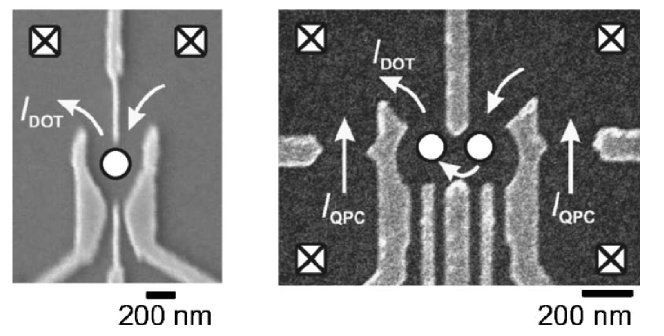
Figure 4: Scanning electron micrographs of a single (left) and double (right) quantum dot. The electrons are confined to the regions indicated by the white circles, surrounded by metallic top gates (light gray areas), and the square boxes indicate the Ohmic contacts. In the double dot setup, two quantum point contacts used for charge sensing can be seen. (Reprinted figures with permission from ref. [40]. Copyright (2007) by the American Physical Society.)

The metallic gates allow one to control the potentials $V_{i}$, which determine the ground-state occupation denoted by $(N_{1},N_{2})$. The spin qubits are realized by occupying each dot with exactly one electron. While control of the electron number down to single occupancy was achieved early on for other types of dots (e.g., vertical quantum dots [111]), the lateral confinement tends to suppress the tunneling rates with the reservoirs. This problem leads to difficulties in observing the few-electron regime but can be overcome by designing proper gating structures (figure 4 shows two examples of actual samples). For this reason, the first demonstrations of few-electron single [112] and double dots [113, 114, 115] with lateral gating are much more recent than for vertical dots.

3.2 Initialization of the spin state

A straightforward procedure to initialize a systems of qubits is to apply a sufficiently large magnetic field and wait for relaxation to the ground state $|{\uparrow\uparrow\uparrow}\ldots\rangle$ to occur. Experiments are usually performed in dilution refrigerators with base temperature around 20 mK, which is smaller than typical Zeeman splittings ($\sim 300$ mK at $B={1~{}\rm T}$ and using the bulk value $g=-0.44$). The initialization time is of the order of a few relaxation times, which in GaAs dots have been reported to be as high as $\sim 1~{}{\rm s}$ (see subsubsect. 3.3.3 for a more complete discussion). In the following, we discuss several other techniques used in practice to initialize single and double GaAs quantum dots to configurations other than $|{\uparrow\uparrow}\rangle$. This allows, e.g., for more flexibility in the subsequent manipulation of the double dot spin state.

3.2.1 Singlet-triplet transition in single dots

We consider here an isolated dot (more precisely, the $i=2$ dot in eq. (18)) and show that, if two electrons are present, the ground state can be chosen to be either a singlet or a triplet, depending on the value of the external magnetic field. Initialization in the desired spin state can, in principle, be accomplished easily by energy relaxation. We start from the lowest energy single electron states with charge configuration (0,1). Clearly, they only differ due to the spin and have energies $E_{\pm}(0,1)=\epsilon_{0}-eV_{2}\mp\Delta E_{Z}/2$ (see eqs. (18) and (19)), where $\Delta E_{Z}=|g\mu_{B}B|$ is the Zeeman splitting. If now one more electron is added, singlet and triplet states can be formed. The lowest lying states are denoted by $S(0,2)$ and $T_{m}(0,2)$, where the subscript $m=0,+,-$ refers to the component of the total spin parallel to ${\bf B}$. The energies are given by $E_{S}(0,2)=2(\epsilon_{0}-eV_{2})+U$ and $E_{T_{m}}(0,2)=E_{S}(0,2)+\Delta E_{ST}-m\Delta E_{Z}$, where the single-triplet splitting at zero magnetic field is given by $\Delta E_{ST}=\Delta\epsilon_{orb}-\Delta U$. Here, $\Delta\epsilon_{orb}=\epsilon_{1}-\epsilon_{0}$ is the difference in orbital energies, which would be the only contribution to $\Delta E_{ST}$ according to the simple charging Hamiltonian eq. (18). However, the splitting is experimentally found to be smaller than $\Delta\epsilon_{orb}$ due to a change $\Delta U$ in the charging energy [40]. The splitting $\Delta E_{ST}$ is generally still positive, resulting in a singlet ground state at zero magnetic field.

Interestingly, the Zeeman energy is smaller than $\Delta E_{ST}$ for typical values of the magnetic field. Therefore, an in-plane magnetic field cannot induce a singlet-triplet transition since, as a good approximation, it does not affect the orbital states. Instead, a significant decrease of $\Delta\epsilon_{orb}$ and increase of $\Delta U$ is produced by a magnetic field $B_{\perp}$ perpendicular to the 2DEG due to orbital effects. The energy crossing of singlet and triplet is typically realized around $B_{\perp}^{0}\simeq 1$ T [116, 117]. This condition is required for the realization of the parity gate discussed in subsubsect. 2.6.1. Furthermore, $B_{\perp}^{0}$ can be tuned via electric gates [117]. In the following, however, we will usually neglect orbital effects of the magnetic field, supposing $\bf B$ to be either in-plane or sufficiently small.

3.2.2 Pauli spin blockade in double dots

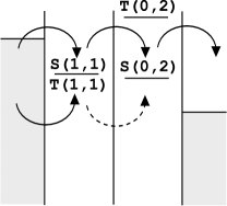
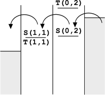
Figure 5: In the left panel, the Pauli spin blockade is illustrated. At positive bias, an electron from the left reservoir can tunnel to the right contact only if it enters the (0,1) double dot in a singlet configuration $S(1,1)$, while the triplet $T(1,1)$ is blocked due to spin conservation (dashed transition). At negative bias the electron can only tunnel in the $S(0,2)$ singlet and transport is always possible. The position of the chemical potentials $\mu_{\alpha}(1,1)$ ($\alpha=S,T_{m}$) is indicated in the first dot, while $\mu_{S}(0,2)$ and $\mu_{T_{m}}(0,2)$ are shown in the second one. The detailed structure of the (1,1) and $T(0,2)$ levels is not specified, since it is of an energy scale much smaller than the $S(0,2)$-$T(0,2)$ singlet-triplet splitting (see subsubsect. 3.2.3 for a more detailed discussion).

The lowest-lying (1,1) spin states are the singlet $S(1,1)$ and the triplets $T_{m}(1,1)$. The energies $E_{\alpha}(1,1)$ (where $\alpha=S$, $T_{m}$) are degenerate in first approximation and eq. (18) gives $E_{\alpha}(1,1)\simeq E(1,1)=2\epsilon_{0}-e(V_{1}+V_{2})+U_{12}$. It is however possible to selectively prepare the system in a triplet state via Pauli spin blockade [118, 119]. This is realized at positive bias if the chemical potentials $\mu_{\alpha}(1,1)$ and $\mu_{\alpha}(0,2)$ of the double dot are adjusted as shown in the left panel of fig. 5. The chemical potentials with respect to the $(0,1)$ occupation are defined as $\mu_{\alpha}(0,2)=E_{\alpha}(0,2)-E(0,1)$ and $\mu_{\alpha}(1,1)=E_{\alpha}(1,1)-E(0,1)$, and are shown in fig. 5 (for simplicity, we neglect the presence of small Zeeman splittings and assume $E_{+}(0,1)\simeq E_{-}(0,1)\equiv E(0,1)$). Tunneling occurs from the left reservoir which is connected to the first dot, to the right reservoir connected to the second dot. The sequence $(0,1)\rightarrow(1,1)\rightarrow S(0,2)\rightarrow(0,1)$ would be energetically allowed both through $S(1,1)$ and $T_{m}(1,1)$, but the transition $T_{m}(1,1)\rightarrow S(0,2)$ is forbidden due to spin conservation. Therefore, as soon as an electron tunnels from the left reservoir to $T_{m}(1,1)$, the double dot is blocked in the triplet state. Transport is only possible after relaxation into $S(1,1)$, which can occur on a millisecond time scale.

Note that at negative bias (cf. the right panel of fig. 5) a finite current can flow through the dots following the sequence $(0,1)\rightarrow S(0,2)\rightarrow S(1,1)\rightarrow(0,1)$. In this case electrons can only tunnel from the right reservoir to a singlet state, since the triplet is too high in energy, and the $T_{m}(1,1)$ states are never involved. The Pauli spin blockade effect thus leads to current rectification.

3.2.3 Singlet-triplet and charge states mixing in double dots

In the presence of an external magnetic field, the triplet energies are $E_{T_{m}}=E(1,1)-m\Delta E_{Z}$. Therefore, the states $T_{0}(1,1)$ and $S(1,1)$ remain degenerate. However, the magnetic fields on the two dots generally differ slightly due to different nuclear configurations (see subsubsect. 3.3.2 on the hyperfine interaction). We assume that the value of the magnetic field is $B\pm\Delta B_{N}$ at the left/right dot, where $\Delta B_{N}\sim 2~{}{\rm mT}$. This causes the relevant eigenstates to have spin configuration $|{\uparrow\downarrow}\rangle$ or $|{\downarrow\uparrow}\rangle$ (singlet-triplet mixing), with energies $E_{\uparrow\downarrow(\downarrow\uparrow)}=E(1,1)\mp g\mu_{B}\Delta B_{N}$. A first consequence of this fact is that the Pauli spin blockade discussed above occurs only for a mixture of $T_{\pm}(1,1)$, but not for $T_{0}(1,1)$. The reason is that $T_{0}(1,1)$ rotates to $S(1,1)$ due to the field inhomogeneity $\Delta B_{N}$, which removes the spin blockade since $S(1,1)$ can tunnel to $S(0,2)$. A second consequence is the possibility to initialize the system into the spin configurations $|{\uparrow\downarrow}\rangle$ or $|{\downarrow\uparrow}\rangle$. This requires a more sophisticated procedure relying on mixing of charge states, as described in the following.

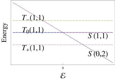
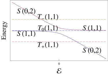
Figure 6: Double-dot energy diagram as a function of the detuning $\varepsilon$, close to $\varepsilon=0$. Without tunneling (left panel) $S(1,1)$ and $T_{0}(1,1)$ are always degenerate, while the $T_{\pm}(1,1)$ are split by a finite magnetic field. At $\varepsilon=0$, the two singlet states $S(1,1)$ and $S(0,2)$ are also degenerate. Inter-dot tunneling (right panel) causes mixing of the $S(1,1)$ and $S(0,2)$ states. The effect of a small difference $\Delta B_{N}$ in the nuclear fields of the two dots is not shown here, and is only relevant when the splitting between $S(1,1)$ and $T_{0}(1,1)$ is small (i.e., in the left panel (independent of $\varepsilon$) and at large detuning ($|\varepsilon|\gg 0$) in the second one). Then, the appropriate eigenstates have spin $|{\uparrow\downarrow}\rangle$ and $|{\downarrow\uparrow}\rangle$, as discussed in the text.

For simplicity, we neglect for the moment the small field inhomogeneity due to $\Delta B_{N}$. We also define the detuning $\varepsilon$ of the local potentials at the two dots as follows: $eV_{1}=e\tilde{V}_{1}-\varepsilon/2$ and $eV_{2}=e\tilde{V}_{2}+\varepsilon/2$, where the $\tilde{V}_{i}$ are constant potentials such that $S(1,1)$ and $S(0,2)$ are degenerate at $\varepsilon=0$. The detuning $\varepsilon$ changes the energy of the (0,2) singlet, $E_{S}(0,2)=E_{S}(1,1)-\varepsilon$, while $E_{S}(1,1)$ and other (1,1) states are not affected. These double dot levels are shown in the left panel of fig. 6, while the triplet states $T_{m}(0,2)$ have much higher energy and are thus not depicted. Consider next the effect of tunneling in the vicinity of $\varepsilon=0$. The tunneling Hamiltonian $H_{T}$ has a matrix element $\langle S(1,1)|H_{T}|S(0,2)\rangle=\sqrt{2}t_{c}$ and causes mixing of the singlets with different charging configurations. At $\varepsilon=0$ perfect mixing is realized, with energy splitting $2\sqrt{2}t_{c}$, while at large $\varepsilon$ the unperturbed eigenstates $S(0,2)$ and $S(1,1)$ are recovered. At large positive detuning, $S(0,2)$ is lower in energy than the $T_{+}(1,1)$ state, and initialization can hence be performed via energy relaxation. If one then slowly changes $\varepsilon$ toward negative values, the system evolves adiabatically along the lower singlet branch into the $S(1,1)$ state (cf. the right panel of fig. 6). The leakage to the $S(0,2)$ state is estimated in ref. [41]. Note also that $T_{+}(1,1)$ is not mixed with the singlet in this simple model.

We now consider the effect of $\Delta B_{N}$, which is important whenever the $S-T_{0}$ splitting is small. Since it usually holds that $t_{c}\gg|g\mu_{B}\Delta B_{N}|$, this is only the case if the detuning becomes large in magnitude. In this limit the splitting goes to zero (see fig. 6) and the inhomogeneity becomes the dominant effect. If the detuning $\varepsilon$ is decreased from large positive to large negative values faster than the time scale determined by $\Delta B_{N}$, the system will be initialized to $S(1,1)$ and will then begin to oscillate between $S(1,1)$ and $T_{0}(1,1)$ with frequency $2g\mu_{B}\Delta B_{N}/h$. Instead, by adiabatically reducing the value of $\varepsilon$, the system can be initialized to the spin configuration with lower energy, $|{\uparrow\downarrow}\rangle$ or $|{\downarrow\uparrow}\rangle$, depending on the sign of $\Delta B_{N}$.

3.3 Relaxation and decoherence in GaAs dots

The requirement of sufficiently long coherence times is perhaps the most challenging aspect for quantum computing architectures in the solid state. It requires a detailed understanding of the different mechanisms that couple the electron’s spin to its environment. We introduce here the main concepts relevant for GaAs dots, while a detailed discussion is postponed to sect. 4.

3.3.1 Spin-orbit coupling

While fluctuations in the electrical environment do not directly couple to the electron spin, they become relevant for spin decoherence in the presence of spin-orbit interaction. In GaAs 2DEGs two types of spin-orbit coupling (Dresselhaus and Rashba) are present. The Dresselhaus spin-orbit coupling originates from the bulk properties of GaAs [120]. The zinc-blend crystal structure has no center of inversion symmetry and a term of the type $H^{3D}_{D}\propto p_{x}(p_{y}^{2}-p_{z}^{2})\sigma_{x}+p_{y}(p_{z}^{2}-p_{x}^{2})\sigma_{y}+p_{z}(p_{x}^{2}-p_{y}^{2})\sigma_{z}$ is allowed in three dimensions, where ${\bf p}$ is the momentum operator and $\boldsymbol{\sigma}$ are the Pauli matrices. Due to the confining potential along the $z$-direction, we can substitute the $p_{z}$ operators with their expectation values. Using $\langle p_{z}^{2}\rangle\neq 0$ and $\langle p_{z}\rangle=0$, one obtains

$$H_{D}=\beta(p_{y}\sigma_{y}-p_{x}\sigma_{x}).$$ (20)

Smaller terms cubic in ${\bf p}$ have been neglected, which is justified by the presence of strong confinement.

The Rashba spin-orbit coupling is due to the asymmetry of the confining potential [121] and can be written in the suggestive form $H_{R}\propto(\boldsymbol{\mathcal{E}}\times{\bf p})\cdot\boldsymbol{\sigma}$, where ${\boldsymbol{\mathcal{E}}}=\mathcal{E}\hat{z}$ is an effective electric field along the confining direction:

$$H_{R}=\alpha(p_{x}\sigma_{y}-p_{y}\sigma_{x}).$$ (21)

The Rashba and Dresselhaus terms produce an internal magnetic field linear in the electron momentum defined by ${\bf B}_{SO}=-2[(\beta p_{x}+\alpha p_{y}){\bf e}_{x}-(\beta p_{y}+\alpha p_{x}){\bf e}_{y}]/g\mu_{B}$. If $\beta=0$, the magnitude of ${\bf B}_{SO}$ is isotropic in ${\bf p}$ and the direction is always perpendicular to the velocity. While moving with momentum ${\bf p}$, the spin precesses around ${\bf B}_{SO}$ and a full rotation is completed over a distance of order $\lambda_{SO}=|\hbar/(\alpha m^{*})|=1-10~{}\mu{\rm m}$, where $m^{*}$ is the effective mass. Generally, Rashba and Dresselhaus spin-orbit coupling coexist, their relative strength being determined by the confining potential. This results in the anisotropy of the spin-orbit coupling in the 2DEG plane (e.g., of the spin splitting as function of ${\bf p}$). In this case, two distinct spin-orbit lengths can be introduced

$$\lambda_{\pm}=\frac{\hbar}{m^{*}(\beta\pm\alpha)}.$$ (22)

For GaAs quantum dots, the spin-orbit interaction is usually a small correction that can be treated perturbatively since the size of the dot (typically $\sim 100$ nm) is much smaller than the spin-orbit coupling lengths $\lambda_{\pm}$. The qualitative effect introduced by the spin-orbit coupling is a small mixing of the spin eigenstates. As a consequence, the perturbed spin eigenstates can be coupled by purely orbital perturbation even if the unperturbed states have orthogonal spin components. Relevant charge fluctuations are produced by lattice phonons, surrounding gates, electron-hole pair excitations, etc. with the phonon bath playing a particularly important role (see subsect. 4.1).

3.3.2 Hyperfine interaction

The other mechanism for spin relaxation and decoherence that has proved to be effective in GaAs dots, and ultimately constitutes the most serious limitation of such systems, is due to the nuclear spins bath. All three nuclear species ⁶⁹Ga, ⁷¹Ga, and ⁷⁵As of the host material have spin 3/2 and interact with the electron spin via the Fermi contact hyperfine interaction

$$H_{HF}={\bf S}\cdot\sum_{i}A_{i}{\bf I}_{i},$$ (23)

where $A_{i}$ and ${\bf I}_{i}$ are the coupling strengths and the nuclear spin operator at site $i$, respectively. The density of nuclei is $n_{0}=45.6~{}{\rm nm}^{-3}$ and there are typically $N\sim 10^{6}$ nuclei in a dot. The strength of the coupling is proportional to the electron density at site $i$, and one has $A_{i}=A|\psi({\bf r}_{i})|^{2}/n_{0}$, where $\psi({\bf r})$ is the orbital envelope wave function of the electron and $A\approx 90~{}\mu$eV.

The study of the hyperfine interaction (23) represents an intricate problem involving subtle quantum many-body correlations in the nuclear bath and entangled dynamical evolution of the electron’s spin and nuclear degrees of freedom. While these topics will be discussed much more deeply in subsect. 4.2, it is nevertheless useful to present here a qualitative picture based on the expectation value of the Overhauser field ${\bf B}_{N}=\sum_{i}A_{i}{\bf I}_{i}/g\mu_{B}$. This field represents a source of uncertainty for the electron dynamics, since the precise value of ${\bf B}_{N}$ is not known. Due to the fact that the nuclear spin bath is in general a complicated mixture of different nuclear states (see subsubsect. 4.2.1 for a more detailed discussion of the nuclear density matrix), the operator ${\bf B}_{N}$ in the direction of the external field ${\bf B}$ does not correspond to a well-defined eigenstate, but results in a statistical ensemble of values. These fluctuations have an amplitude of order $B_{N,max}/\sqrt{N}\sim 5$ mT since the maximum value of $B_{N}$ (with fully polarized nuclear bath) is about 5 T.

Finally, even if it were possible to prepare the nuclei in a specific configuration (e.g., $|{\uparrow\uparrow\downarrow\uparrow}\ldots\rangle$), the nuclear state would still evolve in time to a statistical ensemble on a time scale $t_{nuc}$. Although direct internuclear interactions are present (e.g., magnetic dipole-dipole interactions between nuclei), the most important contribution to the bath’s time evolution is in fact due to the hyperfine coupling itself, causing the back action of the electron spin on the nuclear bath. Estimates of the nuclear bath timescale lead to $t_{nuc}=10-100~{}\mu$s or longer at higher values of the external magnetic field ${\bf B}$ [40].

3.3.3 Relevant time scales

We provide here a summary of the relevant time scales for spin decoherence in GaAs dots. In the Bloch phenomenological description of the time evolution, the spin density matrix $\rho=(1+{\bf P}\cdot\boldsymbol{\sigma})/2$ (where ${\bf P}$ is the spin polarization) satisfies

$$\dot{\bf P}=\frac{g\mu_{B}}{\hbar}{\bf B}\times{\bf P}-\boldsymbol{\Gamma}({\bf P}-{\bf P}_{0}),$$ (24)

where the tensor $\Gamma_{ij}$ is diagonal in a reference frame with the $z$-axis along $\bf B$. With this choice, the equilibrium polarization is ${\bf P}_{0}=P_{0}{\bf e}_{z}$. The time $T_{1}=\Gamma_{zz}^{-1}$ is the longitudinal spin decay time, or spin-flip time, and describes the energy relaxation to the ground state. In GaAs quantum dots $T_{1}$ has a strong magnetic field dependence and can be very long, ranging from $1$ ms around $5~{}{\rm T}$ to more than 1 s at $1~{}{\rm T}$ [123]. This dependence originates entirely from the spin-orbit interaction since, at such high values of the magnetic field, the hyperfine coupling plays no role for energy relaxation (due to the large mismatch between the nuclear and electron Zeeman energies). At small magnetic fields the spin-orbit coupling becomes ineffective and, in fact, does not cause any relaxation at $B=0$ [124]. Nevertheless, the hyperfine interaction contributes to the reduction of $T_{1}$ to much smaller values (down to $10-100$ ns, due to electron-nuclear flip-flops [40]).

The transverse spin decay time $T_{2}=\Gamma_{xx}^{-1}=\Gamma_{yy}^{-1}$ describes the decay of the transverse polarization components $P_{x}$ and $P_{y}$. The $T_{2}$ time cannot be larger than $2T_{1}$. This maximal value is obtained if only the spin-orbit coupling were present [124]. However, $T_{2}$ is dominated by the hyperfine interaction and is much shorter than $T_{1}$. Due to the fluctuations of the Overhauser field in the nuclear bath’s initial state, a transverse decay time of order $10$ ns is obtained (see subsubsect. 4.2.1). In this case, it is clear that the much longer timescale $t_{nuc}=10-100~{}\mu$s does not play a role for the transverse electron spin evolution. This decay time is usually denoted as $T_{2}^{*}$ and referred to as ’ensemble-averaged’ transverse spin decay time. We note that the decoherence process is generally non-exponential (see subsubsect. 4.2.1).

If the initial nuclear state is prepared in an eigenstate of the Overhauser field in the ${\bf B}$ direction, an ’intrinsic’ decay time $T_{2}$ is obtained. A technique for narrowing the initial nuclear state was proposed in ref. [63] and is discussed in subsubsect. 4.2.3. The decay time $T_{2}$ is determined in this case by the coupled dynamics of the electron spin and the nuclear bath. It is comparable to the $t_{nuc}$ time scale (estimates give $T_{2}\sim 1-100~{}\mu$s) and therefore much longer than $T_{2}^{*}$. However, $T_{2}$ is clearly very difficult to access experimentally. A quantity more easily measured is the spin echo decay time $T_{echo}$. We refer to ref. [125] for a description of the spin echo technique, and to ref. [61] for its application to GaAs double dots. This method can be used to perfectly refocus an ensemble of spins in the idealized case where decoherence is only due to static fluctuations of the environment. However, in reality the initial polarization cannot be completely recovered due to the time evolution of the nuclear bath. A decay time $T_{echo}>1~{}\mu$s is reported in ref. [61] at 100 mT.

3.4 Universal quantum gates

Both single- and two-qubit gates have been demonstrated in GaAs quantum dots. The single gate was realized in ref. [126] by means of the well-known electron spin resonance (ESR), which we briefly describe here (for a more extended discussion see, e.g., ref. [125]). An oscillating magnetic field is applied in the transverse direction (perpendicular to $\bf B$) at the resonant frequency $\omega=\Delta E_{Z}/\hbar$. This ESR field can be seen as a sum of two contributions, rotating clockwise and counterclockwise around $\bf B$ at the same frequency $\omega$. However, only the contribution precessing in resonance with the electron spin is of relevance. We denote this component by ${\bf B}_{1}$, while the counter-propagating field is neglected in the following.

Consider now the effect on the electron spin. Without the ESR signal, the spin simply precesses around ${\bf B}$ with angular frequency $\omega$. It is useful to introduce a reference frame rotating around ${\bf B}$ in which the precessing spin appears static. We now apply ${\bf B}_{1}$, which also appears static in the rotating frame. The effect is to induce a precession of the spin around ${\bf B}_{1}$ in the rotating frame. In particular, if the spin is initialized along $\bf B$, a complete spin-flip is realized after a time $\pi\hbar/g\mu_{B}B_{1}$. Typical fields in the experimental setup [126] are up to $\sim 100$ mT, which gives a $\sim 15$ ns switching time.

On the other hand, the two-qubit swap operation was implemented with a much faster gate duration $\sim 0.5$ ns [61]. The gate is realized in a similar way to the original proposal of ref. [7] (see subsect. 2.5), based on the control of the exchange coupling. In practice, the detuning $\varepsilon$ of the double dot is changed, since this modifies the splitting between the lower singlet branch and the triplet $T_{0}$, as described in subsubsect. 3.2.3 and illustrated in fig. 6. If a pulse from a large negative value $\varepsilon_{0}$ to some value $\varepsilon_{c}$ around zero and back to $\varepsilon_{0}$ is applied, a finite energy splitting $J(\varepsilon_{c})$ between triplet $T_{0}$ and singlet $S$ exists for the duration $\tau$ of the pulse. This causes the spin state $|{\uparrow\downarrow}\rangle$ to rotate to $|{\downarrow\uparrow}\rangle$ if the pulse has length $\tau=\pi\hbar/J(\varepsilon_{c})$, which realizes the swap operation. The $\sqrt{\textsc{swap}}$ operation is obtained if the time $\tau$ is half of that required by the swap gate.

3.4.1 Electrical manipulation of individual spins

While standard ESR is useful for single spin manipulation [126] and can in principle be applied to the individual dots of a large array (see subsect. 2.5), it is much more convenient to perform coherent spin rotations through the electric gates at the individual dots. An example of such a technique is the electric-dipole-induced spin resonance (EDSR), which is well known in two dimensions [127, 128, 129] and was also studied in lower dimensional-systems [130, 131]. EDSR in quantum dots was investigated theoretically in ref. [131], which discusses in detail the effect on the electron spin of an external ac electric field mediated by the spin-orbit interaction. In the following, we review the main results of this analysis.

The single dot is described by the two-dimensional Hamiltonian

$$H=\frac{{\bf p}^{2}}{2m^{*}}+U({\bf r})+H_{SO}+H_{Z}-e{\bf E}_{0}\cdot{\bf r}\sin(\omega t),$$ (25)

where ${\bf r}=(x,y)$ is the electron’s coordinate. The second term is the lateral confining potential of the dot and the third term is the spin-orbit coupling (Rashba and Dresselhaus) discussed in subsubsect. 3.3.1. For the present section, it is convenient to define new axes ${\bf e}_{x}=({\bf a}_{x}+{\bf a}_{y})/\sqrt{2}$, ${\bf e}_{y}=-({\bf a}_{x}-{\bf a}_{y})/\sqrt{2}$, and ${\bf e}_{z}={\bf a}_{z}$ (instead of ${\bf e}_{i}={\bf a}_{i}$, as in subsubsect. 3.3.1), where ${\bf a}_{i}$ are unit vectors along the cubic axes of the crystal. With this choice, $H_{SO}$ takes the particularly simple form

$$H_{SO}=\frac{\hbar}{m^{*}}\left(\frac{p_{y}\sigma_{x}}{\lambda_{-}}+\frac{p_{x}\sigma_{y}}{\lambda_{+}}\right),$$ (26)

where $\lambda_{\pm}$ are the spin-orbit lengths defined in eq. (22). The third term in eq. (25) is the usual Zeeman coupling $H_{Z}=g\mu_{B}{\bf B}\cdot{\bf S}$ and the last term is the external electric perturbation. The electric field is assumed to be spatially uniform on the small region of the dot.

The unperturbed states are the eigenstates $\psi_{m}({\bf r})|\pm\rangle$ of the dot Hamiltonian $H_{d}={\bf p}^{2}/2m^{*}+U({\bf r})$. To calculate the effect of the oscillating electric field, one has to resort to third order perturbation theory since the final result has to be proportional to the spin-orbit coupling as well as to the electric field and to the Zeeman splitting $\Delta E_{Z}$. No spin-electric coupling can be obtained at $B=0$, a property related to the invariance of $H_{SO}$ upon time-reversal. It is convenient to approach the problem by making use of the unitary Schrieffer-Wolff transformation $e^{S}He^{-S}$ described in the Appendix. If the confining potential is harmonic, i.e., $U({\bf r})=\frac{1}{2}m^{*}\omega_{0}^{2}r^{2}$, the final result is obtained explicitly as $S=i\boldsymbol{\xi}\cdot\boldsymbol{\sigma}-i\frac{g\mu_{B}}{m^{*}\hbar\omega_{0}^{2}}({\bf B}\times\boldsymbol{\zeta})\cdot\boldsymbol{\sigma}$, where $\boldsymbol{\xi}=(y/\lambda_{-},x/\lambda_{+},0)$, $\boldsymbol{\zeta}=(p_{y}/\lambda_{-},p_{x}/\lambda_{+},0)$, and the spin Hamiltonian for the ground state reads

$$H_{\rm eff}=g\mu_{B}{\bf B}\cdot{\bf S}+g\mu_{B}{\bf h}_{0}\cdot{\bf S}\sin(\omega t),$$ (27)

where

$${\bf h}_{0}=2{\bf B}\times{\bf\Omega}=\frac{2e}{m^{*}\omega_{0}^{2}}{\bf B}\times\left(\frac{E_{0,y}}{\lambda_{-}},\frac{E_{0,x}}{\lambda_{+}},0\right).$$ (28)

Equation (27) clearly reveals the possibility to perform ESR-type spin manipulation, since the electric field induces an effective oscillating magnetic field ${\bf h}_{0}\sin(\omega t)$. From the above expression, we estimate ${\bf h}_{0}\simeq 2~{}{\rm mT}$, using $B=1~{}{\rm T}$, $\lambda_{\pm}=10~{}\mu$m, and $E_{0}=100~{}{\rm V/cm}$. This value is in agreement with a recent experiment [132], in which a spin-flip time around $100$ ns has been found. Corrections to the linear spin-orbit coupling and to the harmonic approximation of the confining potential are also considered in ref. [131] and are responsible for an additional contribution to the EDSR signal which is not discussed here. This additional term only exists in combination with orbital effects of the magnetic field and is absent for an in-plane field ${\bf B}$ (as realized in ref. [132]).

Finally, we note that EDSR is not the only method for spin manipulation via oscillating electric fields. Spin-electric coupling can be also realized by oscillating the position of the dot in the presence of a static but inhomogeneous magnetic field, e.g., provided by the stray field of a nearby micromagnet [133]. This proposal was recently realized in ref. [134]. Gate-induced coherent single spin-rotations were also reported in [135] with a setup very similar to that of the EDSR experiment of ref. [132]. In that case however, the magnetic field is applied in the $[1\bar{1}0]$ direction, perpendicular to the electric field modulation, and eq. (28) gives ${\bf h}_{0}=0$. Therefore, the spin-electric coupling in ref. [135] was attributed to the inhomogeneous Overhauser field produced by the hyperfine interaction.

3.5 Readout of electron spin states

Several methods are available for reading out the spin state of single and double quantum dots and all of them rely on the mechanism of spin-to-charge conversion. While the electron’s magnetic moment is too small to be directly detected, the charge configuration of the single or double dot system can be measured accurately. This is usually accomplished by means of one or more quantum point contacts adjacent to the dots (these are narrow constrictions of the 2DEG through which current can flow), as shown in the right sample in fig. 4. The conductance of a point contact is quantized and is, at the transition between two plateaus, highly sensitive to the electrostatic environment, in particular to the charge distribution in the quantum dots (see the upper right panel in fig. 7). For example, a general strategy for spin readout consists in tuning the system to a configuration in which tunneling between different charge states is allowed or suppressed, depending on the particular spin state. The occurrence of the tunneling process is monitored by the point contact signal, and the corresponding spin state is inferred. We discuss below some more specific examples.

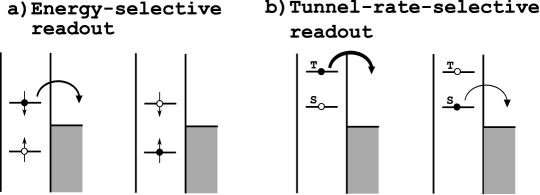
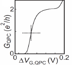
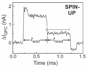
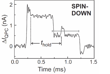
Figure 7: Spin readout in a single dot. In the upper left panels, two possible configurations of the dot are shown, which allow to distinguish between the spin states of the ground and excited levels. In (a) only an electron in the excited state can tunnel out, which is useful for the readout of Zeeman-split states in a single electron dot. In (b) one of the two states (here, the excited state) happens to have a much larger tunneling rate. This configuration is useful for discriminating singlet and triplet states in two-electron dots. In the upper right panel, the conductance of a point contact is shown as a function of the voltage of an adjacent gate. The cross marks the most sensitive position for charge detection. In the bottom panels, an example of the point contact current signal for energy selective readout is shown: The actual measurement is performed in the $t_{\rm read}$ interval (marked in both panels by the horizontal threshold bar), during which the dot is as in (a). In the bottom right panel, a signal above threshold is detected as long as the dot is empty. This corresponds to the spin-$|{\downarrow}\rangle$ electron tunneling out of the dot, followed by tunneling in of an $|{\uparrow}\rangle$ electron. In the left panel, conversely, the dot is always occupied by an electron in the $|{\uparrow}\rangle$ state. The point contact signal before $t_{\rm read}$ refers to the initialization of the dot. See, e.g., ref. [40] for greater detail. (The top right and the two bottom figures are reprinted with permission from ref. [40]. Copyright (2007) by the American Physical Society.)

3.5.1 Single dot readout

The first method for single-shot spin detection we will address here is the so called energy-selective readout [136]. The chemical potentials of the single dot are aligned with the 2DEG reservoir such that the $|{\uparrow}\rangle$ ground state is blocked while a $|{\downarrow}\rangle$ electron can still tunnel out (see fig. 7). Whether the electron leaves the dot or not is ascertained through charge sensing. It was proposed in [137, 138] to demonstrate the ESR rotation of a single spin by making use of this method. Note, however, that the Zeeman splitting must be much larger than the thermal broadening, which implies large ESR excitation frequencies in the microwave range. This has caused additional problems, e.g., photon-assisted tunneling out of the dot, that are difficult to overcome experimentally and prevented this type of experiment from succeeding. Instead, the ESR experiment was performed in double dots using another type of spin readout, which we discuss in the next section. We would also like to mention that another detection method exists for single dots in the case where there is a large difference between the tunneling rates of two states [139]. This method is useful to discriminate singlet and triplet states in a two-electron dot (i.e., the $S(0,2)$ and $T_{m}(0,2)$ discussed in subsubsect. 3.2.1), since the excited triplet has a more extended orbital wave function and better contact with the 2DEG reservoir.

3.5.2 Spin readout in double dots

The mechanisms used for readout of double-dot states are identical to those described for initialization in subsubsects. 3.2.2 and 3.2.3. For example, if a double dot is in the charge configuration (1,1), tunneling to $S(0,2)$ is only possible if the spin state is $|{\uparrow\downarrow}\rangle$ or $|{\downarrow\uparrow}\rangle$. Again, the (1,1) and (0,2) states are easily distinguished by charge sensing. This method of spin readout is used in the ESR experiment of ref. [126]: First, the double dot is initialized to a mixture of $T_{+}(1,1)$ and $T_{-}(1,1)$ via Pauli spin blockade (see left panel of fig. 5). The system is then brought to the Coulomb blockade regime by decreasing the detuning $\varepsilon$. As a consequence, the chemical potential $\mu_{S}(0,2)$ becomes higher than $\mu_{\alpha}(1,1)$ and tunneling is not allowed. The ESR signal can now be applied to one of the two electrons, thereby rotating the initially parallel spin configuration ($|{\uparrow\uparrow}\rangle$ or $|{\downarrow\downarrow}\rangle$) to the antiparallel states $|{\uparrow\downarrow}\rangle$ or $|{\downarrow\uparrow}\rangle$. The double dot is finally brought again to the Pauli spin blockade regime and tunneling can now occur. Repeating the procedure many times, the probability that the single spin was rotated during the application of the ESR signal is determined.

Another detection method can be used in the (1,1) charge configuration to distinguish $|{\uparrow\downarrow}\rangle$ from $|{\downarrow\uparrow}\rangle$: Consider fig. 6, and suppose that at large negative detuning the system is in one of the two states $|{\uparrow\downarrow}\rangle$ or $|{\downarrow\uparrow}\rangle$. By adiabatically changing the detuning to large positive values, $|{\uparrow\downarrow}\rangle$ evolves to $S(0,2)$ and $|{\downarrow\uparrow}\rangle$ to $T_{0}(1,1)$ (for definiteness, we assume here and in the following $\Delta B_{N}>0$) and the two different charge configurations can be distinguished. We can now describe the experiment realizing the $\sqrt{\textsc{swap}}$ operation [61] in greater detail: The system is first initialized in $|{\uparrow\downarrow}\rangle$ as described in subsubsect. 3.2.3. A pulse in $\varepsilon$ is then applied, which introduces a large singlet-triplet splitting, as discussed in subsect. 3.4. The swap or $\sqrt{\textsc{swap}}$ operations are realized for appropriate pulse lengths, but for an arbitrary pulse the double dot is brought, at large negative detuning, into a superposition of $|{\uparrow\downarrow}\rangle$ and $|{\downarrow\uparrow}\rangle$. Finally, the detection method described above is applied and, repeating this scheme many times, the probabilities of the two spin states are measured. Singlet-triplet spin echo experiments can be also performed with a similar procedure [61].

4 Relaxation and spin decoherence in GaAs quantum dots

Electron spins in GaAs quantum dots are inevitably coupled to the surrounding environment. This coupling results in decoherence, which is the process leading to the loss of information stored in a qubit. While an introduction to the mechanisms behind decoherence of electron spins in GaAs quantum dots has already been presented in subsect. 3.3, we will review this topic here in much greater detail. For the reader’s convenience, we will initially repeat some of the basic concepts with additional remarks required for the subsequent treatment.

As already mentioned in subsubsect. 3.3.3, two time scales describing the decoherence process of a single spin can be distinguished. The spin-flip time (also called longitudinal spin decay time) $T_{1}$ describes the time scale for random spin-flips $\left|\uparrow\right>\leftrightarrow\left|\downarrow\right>$, whereas the transverse spin decay time $T_{2}$ describes the decay of superpositions of spin-up and spin-down states $\alpha\left|\uparrow\right>+\beta\left|\downarrow\right>$. The first time scale $T_{1}$ is important if the qubit is operated as a classical bit. For quantum computing, also the spin decoherence time $T_{2}$ plays a major role and must thus be sufficiently long.

The relaxation time $T_{1}$ and the decoherence time $T_{2}$ are not unrelated. Naively, one might expect $T_{2}\ll T_{1}$, but as shown in [124] and as we will see below, this is not necessarily the case for arbitrarily large Zeeman splittings. In general, the electron spin $\mathbf{S}$ couples both to the external magnetic field $\mathbf{B}$, and to the fluctuating internal field $\mathbf{h}(t)$ with the time-averaged value $\left<\mathbf{h}(t)\right>=0$ (actual sources of this volatile internal field will be discussed later on). We also assume $\left<h_{i}(t)h_{j}(t^{\prime})\right>\propto\delta_{ij}$, where $h_{i}(t)$ with $i=x,y,z$ are the components of the vector $\mathbf{h}(t)$. The Hamiltonian for the single-electron spin reads

$$H=g\mu_{B}\mathbf{S}\cdot\mathbf{B}+\mathbf{S}\cdot\mathbf{h}(t),$$ (29)

where $g$ is the $g$-factor ($g=-0.44$ in bulk GaAs) and $\mu_{B}=9.27\times 10^{-24}$ J/T is the magnetic moment of the single electron spin. The relaxation time can be expressed in the weak coupling limit as [140]

$$\frac{1}{T_{1}}=\frac{1}{2\hbar^{2}}\int_{-\infty}^{\infty}dt~{}\mathrm{Re}\left[\left<h_{x}(0)h_{x}(t)\right>+\left<h_{y}(0)h_{y}(t)\right>\right]e^{-i\omega_{Z}t},$$ (30)

where $\omega_{Z}=g\mu_{B}B/\hbar$ is the Zeeman frequency. On the other hand, the expression for the $T_{2}$ time is

$$\frac{1}{T_{2}}=\frac{1}{2T_{1}}+\frac{1}{2\hbar^{2}}\int_{-\infty}^{\infty}dt~{}\mathrm{Re}\left<h_{z}(0)h_{z}(t)\right>.$$ (31)

Notably, the relaxation contribution $(2T_{1})^{-1}$ has been separated from the dephasing part incorporated in the integral. It was proven that for the spin-orbit interaction (discussed in the next section), up to linear order in momentum, $\mathbf{h}(t)\cdot\mathbf{B}=0$ and the effective magnetic field can only have fluctuations transverse to the applied $\mathbf{B}$-field. As a result, the integral yields zero and the upper bound on $T_{2}$ is realized, i.e., $T_{2}=2T_{1}$, independent of the origin of the fluctuations [124].

In contrast to the single-electron case, experiments performed on an ensemble of systems with different environments are subject to additional decoherence. It is therefore required to introduce an ensemble-averaged transverse spin decay time $T_{2}^{*}$, which is typically much shorter than the transverse single-spin decay time $T_{2}$. One finds various other symbols for $T_{2}^{*}$ in the literature, such as $\tau_{c}$ (the correlation time) and $T_{M}$ (the magnetization envelope decay time), used to emphasize the non-exponential character of the decay. See subsubsect. 3.3.3 for a summary of theoretical estimates and experimental results for these various decoherence time scales.

For quantum computers to work on a large scale, it is crucial to understand the microscopic mechanisms underlying dissipation and decoherence, and to devise effective methods to reduce their impact on the electron’s spin dynamics. This would allow to achieve longer coherence times and, in turn, reduce qubit errors. Two main sources of decoherence in GaAs are to be identified, namely the spin-orbit and the hyperfine interaction. (i) The spin-orbit interaction couples the electron’s spin to its orbital degrees of freedom. The orbital motion is influenced by lattice phonons, which provide a large dissipative bosonic reservoir. In this way, an effective coupling between the electron’s spin and the phonon bath is established leading to energy dissipation and decoherence. (ii) The Fermi contact hyperfine interaction couples the electron’s spin directly to the surrounding bath of fluctuating nuclear spins. In a typical GaAs quantum dot the electron wave function overlaps with wave functions of approximately $10^{5}$ nuclei. The electron spin dynamics is thus strongly affected by the nuclear spin bath. These two decoherence mechanisms will be discussed extensively in the remaining part of this section.

4.1 Spin-orbit interaction

The main features of the spin-orbit interaction have already been discussed in subsubsect. 3.3.1. Here, we would like to emphasize that this interaction originates, in fact, from the relativistic Dirac equation and provides a direct coupling between the spin $\mathbf{S}$ and the momentum $\mathbf{p}$. In vacuum, the spin-orbit term derived from the Dirac equation turns out to be

$$H_{SO}=-\frac{\hbar e}{2m^{2}c^{2}}\mathbf{S}\cdot\left(\mathbf{p}\times{\boldsymbol{\nabla}}V\right),$$ (32)

where $c$ is the speed of light, $m$ is the free electron mass, $e$ the electron charge, $\mathbf{S}=\makebox{\boldmath$\sigma$}/2$ with $\sigma$ being the vector of Pauli matrices, $\mathbf{p}$ is the canonical momentum, and $V$ is an electric potential. Accounting for the lack of spatial inversion symmetry in the bulk GaAs crystal and assuming the presence of an asymmetric confining potential originating in the GaAs/AlGaAs heterostructure, the two-dimensional spin-orbit Hamiltonian reduces to the sum of the Rashba [141] and Dresselhaus [120] contributions

$$H_{SO}=H_{R}+H_{D}=\alpha\left(p_{x}\sigma_{y}-p_{y}\sigma_{x}\right)+\beta\left(p_{x}\sigma_{x}-p_{y}\sigma_{y}\right),$$ (33)

where $\alpha$ is tunable by external gates while $\beta$ is a material constant stemming from the bulk inversion asymmetry. The tunability of $\alpha$ allows one, in principle, to achieve $\alpha=\pm\beta$. In this particular case, $H_{SO}=\alpha\left(p_{x}\mp p_{y}\right)\left(\sigma_{x}\pm\sigma_{y}\right)$ and $\left(\sigma_{x}\pm\sigma_{y}\right)$ is conserved. As a result, the electron’s spin decouples from its momentum degrees of freedom.

4.1.1 Relaxation through phonons

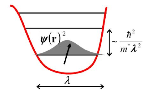
Figure 8: An electron in its orbital ground state, as determined by the two-dimensional confining potential (thick red curve). The probability to find the electron becomes negligible at distances greater than dot’s diameter $\lambda\sim 100~{}{\rm nm}$. The ground state is separated from the first excited state by an energy gap $\sim\hbar^{2}/m^{*}\lambda^{2}$.

We consider in this section the following two-dimensional model Hamiltonian for an electron in the conduction band

$$H=H_{d}+H_{Z}+H_{SO}+H_{el-ph}(t).$$ (34)

Equation (34) above only differs from eq. (25) by the last term. $H_{d}={\bf p}^{2}/2m^{*}+U(\mathbf{r})$ describes the electron in the presence of a lateral confining potential, which is assumed parabolic, i.e., $U(\mathbf{r})=m^{*}\omega_{0}^{2}r^{2}/2$, and determines the ground state orbital wave function $\psi_{0}({\bf r})=\exp(-r^{2}/2\lambda^{2})/\lambda\sqrt{\pi}$, where $\lambda^{-2}=\hbar^{-1}\sqrt{(m^{*}\omega_{0})^{2}+(eB_{z}/2c)^{2}}$. The probability density $|\psi_{0}(\mathbf{r})|^{2}$ to find the electron outside a circle of radius $\lambda/2$ is negligible, where a typical dot diameter is $\lambda\sim 100$ nm (see Figure 8). The second term of eq. (34) is the Zeeman Hamiltonian $H_{Z}=g\mu_{B}\mathbf{B}\cdot{\bf S}$ and the third one is the spin-orbit interaction $H_{SO}$, discussed briefly in the previous section. As discussed for eq. (25), it is convenient to express $H$ in a rotated coordinate system, such that $H_{SO}$ takes the simpler form eq. (26). Note that, for a typical GaAs quantum dot, the spin orbit lengths $\lambda_{\pm}\sim 1-10~{}\mu$m are much larger than the diameter of the dot and the orbital level spacing $\hbar^{2}/m^{*}\lambda^{2}\sim 1$ meV $\approx 10$ K far exceeds typical experimental temperatures $k_{B}T$ and Zeeman energies $g\mu_{B}B$. The last contribution in eq. (34) takes into account two different types of electron-phonon interactions [142]

$$H_{el-ph}(t)=\sum_{\mathbf{q},j}\frac{F(q_{z})e^{i\mathbf{q}_{\parallel}\cdot\mathbf{r}}}{\sqrt{2\rho_{c}\omega_{\mathbf{q},j}/\hbar}}\left(e\beta_{\mathbf{q},j}-iq\Xi_{\mathbf{q},j}\right)\left(b_{-\mathbf{q},j}^{\dagger}+b_{\mathbf{q},j}\right),$$ (35)

where the time-dependence is due to the phonon operators. In the above equation, $b_{\mathbf{q},j}^{\dagger}$ creates an acoustic phonon with wave vector $\mathbf{q}=\left(\mathbf{q}_{\parallel},q_{z}\right)$, branch index $j$, and dispersion $\omega_{\mathbf{q},j}$. Furthermore, $\rho_{c}$ is the sample density and $F(q_{z})=\int_{-\infty}^{+\infty}|\varphi(z)|^{2}e^{iq_{z}z}dz$, where $\varphi(z)$ is the electron wave function in the direction $z$ of the confinement (the full wave function is $\varphi(z)\psi({\bf r})$, where ${\bf r}=(x,y)$). Note that $F(q_{z})$ equals unity for $|q_{z}|\ll d^{-1}$ and vanishes for $|q_{z}|\gg d^{-1}$, where $d$ is the size of the quantum well along the $z$ axis. The couplings $\beta_{\mathbf{q},j}$ are determined by the piezoelectric electron-phonon interaction as follows

$$\beta_{\mathbf{q},j}=\frac{2\pi}{q^{2}\kappa}\beta^{\mu\nu\eta}q_{\mu}\left(q_{\nu}e_{\eta,j}(\mathbf{q})+q_{\eta}e_{\nu,j}(\mathbf{q})\right),$$ (36)

where $\beta^{\mu\nu\eta}$ is the electro-mechanical tensor, $\kappa$ is the dielectric constant, and $e_{\mu,j}(\mathbf{q})$ is the phonon polarization unit vector for branch $j$. For GaAs, $\beta^{\mu\nu\eta}=h_{14}$ if the indices $\mu\nu\eta$ are a cyclic permutation of $xyz$, where $h_{14}\approx 0.16$ C/m². Otherwise, $\beta^{\mu\nu\eta}=0$ [143]. Finally, the deformation potential electron-phonon interaction gives

$$\Xi_{\mathbf{q},j}=\frac{1}{2q}\Xi^{\mu\nu}\left(q_{\mu}e_{\nu,j}(\mathbf{q})+q_{\nu}e_{\mu,j}(\mathbf{q})\right),$$ (37)

where $\Xi^{\mu\nu}$ is the deformation tensor. For GaAs one has $\Xi^{\mu\nu}=\Xi_{0}\delta_{\mu\nu}$, where $\Xi_{0}\approx 7$ eV [143]. Therefore, the above expression simply becomes $\Xi_{\mathbf{q},j}=\Xi_{0}\delta_{j,1}$, since only the longitudinal branch $j=1$ gives a non-vanishing contribution.

As in subsubsect. 3.4.1, it is convenient to approach the perturbative treatment of the Hamiltonian (34) by making use of the unitary Schrieffer-Wolff transformation described in the Appendix. The final result of this procedure is an effective spin Hamiltonian of the form

$$H_{\mathrm{eff}}=\left<\psi_{0}({\bf r})\right|e^{S}He^{-S}\left|\psi_{0}({\bf r})\right>=g\mu_{B}\mathbf{B}\cdot{\bf S}+g\mu_{B}{\bf S}\cdot\delta\mathbf{B}(t)+\ldots,$$ (38)

where spin-independent terms are omitted. In the above equation, $\delta\mathbf{B}(t)=2\mathbf{B}\times\mathbf{\Omega}(t)$ where eq. (93) immediately gives $\mathbf{\Omega}(t)=\left<\psi_{0}({\bf r})\right|[((1-\hat{P})\hat{L}_{d}^{-1}\makebox{\boldmath$\xi$}),H_{el-ph}(t)]\left|\psi_{0}({\bf r})\right>$. The vector $\xi$ and the superoperators $\hat{P}$ and $\hat{L}_{d}^{-1}$ are defined in the Appendix. Note that the form of $H_{\rm eff}$ above is the same as eq. (29). However, as pointed out in the beginning of sect. 4, there can be only transverse fluctuations of the effective magnetic field, i.e., $\delta\mathbf{B}(t)\cdot\mathbf{B}=0$, to first order in the spin-orbit interaction. This property holds not only for phonons, but is valid regardless of the nature of the charge fluctuations, as is seen from the general form of eq. (92).

4.1.2 Energy relaxation

If the scattering events are not correlated, i.e., if the phonons emitted and absorbed by the electron leave the dot in a time $\tau_{c}$ which satisfies $d/s\lesssim\tau_{c}\lesssim\lambda/s$ (with $s$ being the sound velocity), then the expectation value $\left<\mathbf{S}\right>$ obeys the Bloch equation

$$\dot{\left<\mathbf{S}\right>}=g\mu_{B}\mathbf{B}\times\left<\mathbf{S}\right>-\mathbf{\Gamma}\left<\mathbf{S}\right>+\mathbf{\Upsilon}.$$ (39)

In this formula, the decay tensor $\mathbf{\Gamma}$ and the inhomogeneous term $\mathbf{\Upsilon}$ can be derived in the Born-Markov approximation for a generic $\delta\mathbf{B}(t)$ which fulfills $\left<\delta\mathbf{B}(t)\right>=0$, and are expressed in terms of the spectral function

$$J_{ij}(\omega)=\frac{g^{2}\mu_{B}^{2}}{2\hbar^{2}}\int_{0}^{\infty}\left<\delta B_{i}(0)\delta B_{j}(t)\right>e^{-i\omega t}dt.$$ (40)

In general, besides a term proportional to the spectral function $\mathbf{J}$, the tensor $\mathbf{\Gamma}$ receives an additional contribution from elastic scattering of the electron spin. However, because of the transverse nature of the magnetic field fluctuations, this contribution vanishes identically. The final result for $T_{1}$ and $T_{2}$ reads

$$\frac{1}{T_{1}}=\frac{2}{T_{2}}={\rm Re}[J_{xx}(\omega_{Z})+J_{xx}(-\omega_{Z})+J_{yy}(\omega_{Z})+J_{yy}(-\omega_{Z})],$$ (41)

where $\omega_{Z}=g\mu_{B}B/\hbar$ is the Zeeman frequency, as in eq. (30). The explicit expression for $\mathrm{Re}J_{xx}(\omega)$ reads [124]

$$\mathrm{Re}J_{xx}(\omega) = \frac{\omega_{Z}^{2}\omega^{3}(2N_{\omega}+1)}{(2\Lambda_{+}m^{*}\omega_{0}^{2})}\sum_{j=1}^{3}\frac{\hbar}{\pi\rho_{c}s_{j}^{5}}\int_{0}^{\pi/2}d\theta\sin^{3}\theta$$ (42)

$$\times e^{-(\omega\lambda\sin\theta)^{2}/2s_{j}^{2}}\left|F\left(\frac{|\omega|}{s_{j}}\cos\theta\right)\right|^{2}\left(e^{2}\overline{\beta}_{j,\theta}^{2}+\frac{\omega^{2}}{s_{j}^{2}}\overline{\Xi}_{j}^{2}\right)$$

where $N_{\omega}=(e^{\hbar\omega/T}-1)^{-1}$ is the Bose distribution and $s_{j}$ is the velocity of sound for the branch $j$. In GaAs, the $s_{j}$ have values $s_{1}\approx 4.7\times 10^{3}$ m/s and $s_{2}=s_{3}\approx 3.37\times 10^{3}$ m/s. Furthermore, $\overline{\Xi}_{j}=\Xi_{0}\delta_{j,1}$ with $\Xi_{0}\approx 7$ eV, $\overline{\beta}_{1,\theta}=3\sqrt{2}\pi h_{14}\kappa^{-1}\sin^{2}\theta\cos\theta$, $\overline{\beta}_{2,\theta}=\sqrt{2}\pi h_{14}\kappa^{-1}\sin 2\theta$, $\overline{\beta}_{3,\theta}=3\sqrt{2}\pi h_{14}\kappa^{-1}(3\cos^{2}\theta-1)\sin\theta$ with $h_{14}\approx 0.16$ C/m² and $\kappa\approx 13$. The result for $J_{yy}(\omega)$ is obtained by substituting $\Lambda_{+}\to\Lambda_{-}$ in the above expression. Here $\Lambda_{\pm}$ are effective spin-orbit lengths given in [124]. For a magnetic field $\bf B$ in the $z$ direction the simple result $\Lambda_{\pm}=\lambda_{\pm}$ is obtained, where $\lambda_{\pm}$ are defined in eq. (22). Note that both $J_{xx}$ and $J_{yy}$ are multiplied by $\omega^{3}$, thereby exhibiting a super-Ohmic behavior.

By explicitly evaluating this rather cumbersome expression, a relaxation time $T_{1}\approx(825\pm 275)~{}\mu$s is found at $B=8$ T. This result is in very good agreement with the experimental value $T_{1}^{\mathrm{exp}}=800~{}\mu$s at the same strength of the magnetic field [136]. The rather large uncertainty of the theoretical prediction is due to the measured value of the $g$-factor.

4.1.3 Magnetic field dependence of the relaxation rate

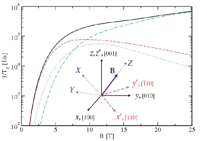
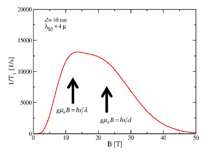
Figure 9: Left panel: The relaxation rate $1/T_{1}$ given by eq. 42 is plotted as a function of the magnetic field $B$. Contributions due to the piezoelectric effect with transverse and longitudinal phonons are plotted as dashed and dotted curves, respectively. The contribution due to the deformation potential mechanisms is shown by a dot-dashed curve. Right panel: The relaxation rate $1/T_{1}$ is plotted for large magnetic fields, where the $1/T_{1}\propto B^{5}$ behavior is suppressed.

Another important result is obtained in the range of magnetic field below $\sim 3$ T, when the relaxation rate $1/T_{1}$ increases with the magnetic field as $B^{5}$. This can be inferred from the presence in eq. (42) of the prefactor $\omega_{Z}^{2}\omega^{3}$ (note that, in the final expression for $1/T_{1}$, one has to set $\omega=\omega_{Z}$). There are three contributions to this power-law behavior: (i) The fluctuating magnetic field is proportional to the external magnetic field, i.e., $\delta B^{2}\propto B^{2}$. (ii) The phonon velocity is proportional to the phonon dispersion, i.e., $v_{ph}(\omega)\propto\omega^{2}$ with $\omega=g\mu_{B}B$. (iii) The spin-orbit Hamiltonian couples to the magnetic field through its momentum, i.e., $H_{SO}\propto p_{\alpha}\propto B$. The final result $\propto B^{5}$ was confirmed experimentally in ref. [123]. In the opposite limit, i.e. for magnetic fields larger than $\sim 12$ T, the power law is suppressed, since phonons are averaged to zero over the dot size $\lambda_{ph}^{B}=s/h\mu_{B}B\ll\lambda$. These two regimes have been summarized in fig. 9.

4.1.4 Magnetic field angular dependence

For an arbitrary direction of the magnetic field $\mathbf{B}=B(\sin\theta\cos\varphi,$ $\sin\theta\sin\varphi,\cos\theta)$ it was found [124] that

$$\frac{1}{T_{1}}=\frac{\left(\alpha^{2}+\beta^{2}\right)\left(1+\cos^{2}\theta\right)+2\alpha\beta\sin^{2}\theta\sin 2\varphi}{\beta^{2}T_{1}(\theta=\pi/2,\alpha=0)}.$$ (43)

Noteworthy, there is an interference between the Rashba and Dresselhaus terms which leads to a diverging relaxation time $T_{1}\rightarrow\infty$ when $\alpha=\beta$, $\theta=\pi/2$, and $\varphi=3\pi/4$. This result is valid to all orders in the spin-orbit interaction and is an effect of spin conservation, which occurs for the special condition $\alpha=\beta$ of the spin-orbit couplings (see also the discussion of $H_{SO}$, earlier in this section).

4.2 Hyperfine interaction

As discussed in the previous section, the relaxation process of the spin polarization in GaAs quantum dots is dominated by the spin-orbit interaction, which couples the electron spin to the phonon bath. If no other effect were present, the upper bound for the decoherence time $T_{2}=2T_{1}$ would be satisfied [124]. Measurements of $T_{1}$ reveal that ultra-long relaxation times $\sim 1$ s are achievable for magnetic fields $B\sim 1$ T [123]. Hence, long decoherence times might be expected as well. Unfortunately, measured spin decoherence times are considerably shorter and range from $1~{}\mu$s [61] to roughly $10~{}\mu$s [126, 144]. Thus, the spin decoherence in GaAs must be dominated by other effects.

The major source of decoherence in GaAs was investigated theoretically in [55] and was attributed to the hyperfine interaction with the nuclear spins. In fact, this is the cause of decoherence in numerous candidate systems for quantum information processing applications such as quantum dots [145, 61, 126], Si:P donors [146], NV centers in diamond [15, 147], and molecular magnets [148, 149].

A possible way to limit this decoherence problem in GaAs might be to use holes instead of electrons [150, 151, 152], since the Fermi contact hyperfine interaction vanishes in this case. The detailed form of the hyperfine interaction for holes was recently studied in ref. [152] and receives contributions from the dipole-dipole interaction and the coupling of the electron orbital angular momentum to the nuclear spins. It is indeed found to be smaller than for electrons (but still sizable) and of Ising type, differently from the electron’s isotropic Heisenberg interaction. Another strategy against decoherence would be to employ materials such as C, Si, Ge and others, which do not host any nuclear magnetic moment. Finally, one can insist on GaAs, which is still the most common material for quantum information processing applications, and deal with the nuclear spins. In this section we follow this last approach and focus on the decoherence process caused by the hyperfine interaction. Based on its detailed understanding, we suggest possible schemes for its reduction or elimination.

The following Hamiltonian describes the hyperfine interaction in a single quantum dot in the presence of a magnetic field applied in $z$ direction $\mathbf{B}=B\mathbf{e}_{z}$ and dipole-dipole interaction $H_{dd}$ between nuclear spins

$$H=\mathbf{h}\cdot\mathbf{S}+bS_{z}+\epsilon\sum_{i}I^{z}_{i}+H_{dd},$$ (44)

where $\mathbf{h}=\sum_{i}A_{i}\mathbf{I}_{i}$ is the nuclear magnetic field also known as the Overhauser field, $A_{i}$ is the hyperfine coupling strength at site $i$, $b=g\mu_{B}B$ is the electron Zeeman splitting and $\epsilon=g_{I}\mu_{N}B$ is the nuclear Zeeman splitting. The nuclear (Bohr) magneton is denoted by $\mu_{I}$ ($\mu_{B}$) and nuclear (electron) $g$-factor by $g_{I}$ ($g$). Typically, the electron orbital energy level spacing for lateral quantum dots containing one electron is much larger than the energy scale of the hyperfine interaction. Therefore, the electron remains in its orbital ground state and no orbital excitations due to the interactions with nuclei are possible.

The hyperfine coupling is non-uniform since we have $A_{i}\propto|\psi(\mathbf{r}_{i})|^{2}$. For GaAs, the average coupling strength weighted by the natural abundance of each isotope (cf. subsubsect. 3.3.2) is $A\approx 90~{}\mu$eV. The typical energy associated with the hyperfine interaction is then $A/N\approx 10^{6}$ s^-1, where $N\approx 10^{5}$ is the typical number of nuclei in contact with the electron spin. This scale has to be compared with the dipole-dipole interaction energy $\left<(\delta H_{dd})^{2}\right>^{1/2}\approx 10^{4}$ s^-1, which is much smaller and will be neglected in the following.

The nuclear Zeeman term can be formally eliminated from the Hamiltonian by transforming to a rotating reference frame [153]. One can also separate the longitudinal part $H_{0}$ from the transverse flip-flop part $V$ of the hyperfine Hamiltonian, which leads to the following expression

$$H^{\prime}=H_{0}+V=(b^{\prime}+h_{z})S_{z}+\frac{1}{2}(h_{+}S_{-}+h_{-}S_{+}),$$ (45)

where $h_{\pm}=h_{x}\pm ih_{y}$ and $S_{\pm}=S_{x}\pm iS_{y}$ are ladder operators for the nuclear field and the electron spin, respectively, and $b^{\prime}=b-\epsilon$. From this representation, it becomes clear that the longitudinal component $V$ describes flip-flop processes: If the electron spin and the spin of a neighboring nucleus are opposite, their direction can be simultaneously swapped. This flip-flop mechanism allows for electron mediated diffusion of the nuclear spins and determines fluctuations of the nuclear spins polarization on a timescale of order $100~{}\mu$s.

4.2.1 Ensemble averaged decoherence time

A central question to address is how the initial state of the nuclei affects the evolution of the electron spin. Assume that for times $t<0$ the electron spin and the nuclear bath are decoupled and described by the density operators $\rho_{S}(0)$ and $\rho_{I}(0)$ respectively. At $t=0$, they are brought into contact over a switching time scale that is sufficiently short, e.g., the time taken to inject an electron into a quantum dot. The initial state of the entire system $\rho(t=0)$ is continuous at $t=0$ and, hence, $\rho(0^{-})=\rho(0^{+})=\rho_{S}(0)\otimes\rho_{I}(0)$. Following ref. [153], we assume for simplicity nuclei with spin-$\frac{1}{2}$ and consider three types of initial spin configurations, namely

$$\rho_{I}^{(1)}(0)=\left|\psi_{I}\right>\left<\psi_{I}\right|\hskip 10.0pt\mathrm{with}\hskip 10.0pt\left|\psi_{I}\right>=\bigotimes_{k=0}^{N}\left(\sqrt{f_{\uparrow}}\left|\uparrow_{k}\right>+e^{i\phi_{k}}\sqrt{1-f_{\uparrow}}\left|\downarrow_{k}\right>\right),$$ (46)

$$\rho_{I}^{(2)}(0)=\sum_{N_{\uparrow}}\binom{N}{N_{\uparrow}}f_{\uparrow}^{N_{\uparrow}}\left(1-f_{\uparrow}\right)^{N-N_{\uparrow}}\left|N_{\uparrow}\right>\left<N_{\uparrow}\right|,$$ (47)

$$\rho_{I}^{(3)}(0)=\left|n\right>\left<n\right|\hskip 20.0pt\mathrm{with}\hskip 10.0pth_{z}\left|n\right>=\sum_{k}A_{k}I_{k}^{z}\left|n\right>=\frac{pA}{2}\left|n\right>,$$ (48)

where $\left|\uparrow_{k}\right>$ and $\left|\downarrow_{k}\right>$ are the spin-up and spin-down eigenstates of the $k$-th nucleus, $f_{\uparrow}$ determines the nuclear polarization $p=2f_{\uparrow}-1$, $\phi_{k}$ is an arbitrary site-dependent phase, $N$ is the total number of nuclei, and $N_{\uparrow}$ is the number of the nuclei in the spin-up state. $\left|N_{\uparrow}\right>$ thus denotes any product state of the form $\left|\uparrow\downarrow\uparrow\uparrow\cdots\right>$ with $N_{\uparrow}$ nuclear spins up and $N-N_{\uparrow}$ spins down, and $A=\sum_{k}A_{k}$.

We note that $\rho_{I}^{(1)}(0)$ and $\rho_{I}^{(3)}(0)$ are both pure states but in the first one $\left|\psi_{I}\right>$ is chosen to render the $z$ component of nuclear spin translationally invariant: $\left<\psi_{I}\right|I_{k}^{z}\left|\psi_{I}\right>=\left(2f_{\uparrow}-1\right)/2=p/2$, while in the second one $\left|n\right>$ is chosen to be an eigenstate of $h_{z}$ with eigenvalue $pA/2$. On the other hand, $\rho_{I}^{(2)}(0)$ is a mixed state, which corresponds to an ensemble of product states where the $N$ spins in each product state are selected from a bath of polarization $p$.

Now we evaluate the nuclear spin dynamics under $H_{0}$, i.e., when the flip-flop term $V$ can be neglected. This is justified, for instance, at large magnetic fields, because the energy gap between spin-up and spin-down states of the electron is much larger than the nuclear splitting between spin-up and spin-down states, thus making the flip-flop transition energetically forbidden. We also assume the simplified case of uniform coupling constants $A_{k}=A/N$. Since $\left[H_{0},S_{z}\right]=0$, $\left<S_{z}\right>_{t}$ is constant. Instead, $[H_{0},S_{\pm}]\neq 0$ and the transverse components, $\left<S_{\pm}\right>_{t}=\left<S_{x}\right>_{t}\pm i\left<S_{y}\right>_{t}$, have a nontrivial time dependence, which can be evaluated by tracing out the electron and nuclear degrees of freedom $\left<S_{\pm}\right>_{t}=\mathrm{Tr}\left[e^{iH_{0}t}S_{\pm}e^{-iH_{0}t}\rho(0)\right]$. The final results read

$$\left<S_{\pm}\right>_{t}^{(1,2)}=\left<S_{\pm}\right>_{0}\sum_{N_{\uparrow}}\binom{N}{N_{\uparrow}}f_{\uparrow}^{N_{\uparrow}}\left(1-f_{\uparrow}\right)^{N-N_{\uparrow}}e^{\pm i\left(b^{\prime}+AM(N_{\uparrow})/2N\right)t},$$ (49)

$$\left<S_{\pm}\right>_{t}^{(3)}=\left<S_{\pm}\right>_{0}e^{\pm i\left(b^{\prime}+pA/2\right)t},$$ (50)

where $M(N_{\uparrow})=2N_{\uparrow}-N$ is the nuclear magnetization on a dot with $N_{\uparrow}$ nuclear spins up and we generally set $\hbar=1$ from now on. Note the similarity between randomly correlated pure states and mixed states, which yield the same final result eq. (49). It is also seen that no decay in eq. (50) is obtained for the eigenstate $|n\rangle$, but a finite transverse relaxation time follows from eq. (49), due to the average over the binomial distribution. One can further evaluate the expression in eq. (49), by direct application of the central limit theorem, and obtain

$$\left<S_{\pm}\right>_{t}^{(1,2)}=\left<S_{\pm}\right>_{0}e^{-t^{2}/2t_{c}^{2}\pm i\left(b^{\prime}+pA/2\right)t}\hskip 10.0pt\mathrm{with}\hskip 10.0ptt_{c}=\frac{2}{A}\sqrt{\frac{N}{1-p^{2}}}.$$ (51)

This Gaussian decay occurs on a timescale $t_{c}\approx 5$ ns, for a GaAs quantum dot with $p^{2}\ll 1$ and $N=10^{5}$.

4.2.2 Electron Spin Resonance

To study the electron spin dynamics, the electron spin resonance (ESR) technique is very fruitful. In order to achieve the resonance condition, an alternating magnetic field $\mathbf{B}_{\mathrm{ac}}=B_{\mathrm{ac}}\mathbf{e}_{x}\cos\omega t$ is applied in the transverse direction, in addition to the static out-of-plane magnetic field $\mathbf{B}=B\mathbf{e}_{z}$. The Hamiltonian of this system is

$$H_{ESR}=(h_{z}+b)S_{z}+b_{1}\cos(\omega t)S_{x},$$ (52)

where $b_{1}=g\mu_{B}B_{\mathrm{ac}}$. The first term is $H_{0}$ of eq. (45), but we neglected the nuclear Zeeman splitting $\epsilon$. We have again assumed that spin-flip processes are not important since the static magnetic field is large. As discussed in the previous section, the nuclear bath is in a superposition of eigenstates $|n\rangle$ of the $h_{z}$ operator, with corresponding eigenvalues $h_{z}^{n}$. The distribution of the $h_{z}^{n}$ eigenvalues is Gaussian, with mean $h_{0}={\rm Tr}\{\rho_{I}h_{z}\}$ and variance $\sigma\sim A/\sqrt{N}$, defined by $\sigma^{2}={\rm Tr}\{\rho_{I}(h_{z}-h_{0})^{2}\}$. As in the previous section, $\rho_{I}$ is the density matrix of the nuclear system.

The decay of the driven Rabi oscillations is found in a rotating-wave approximation (valid for $(b_{1}/b)^{2}\ll 1$) and is given by [63]

$$P_{\uparrow}(t)\sim\frac{1}{2}+C+\sqrt{\frac{b_{1}}{8\sigma^{2}t}}\cos\left(\frac{b_{1}}{2}t+\frac{\pi}{4}\right)+o\left(\frac{1}{t^{3/2}}\right)$$ (53)

where $C=1/2-\left(\sqrt{2\pi b_{1}^{2}}/8\sigma\right)\exp\left(b_{1}^{2}/8\sigma^{2}\right)\mathrm{erfc}\left(b_{1}/\sqrt{8\sigma^{2}}\right)$ is a time-independent constant. The above formula holds for $t\gg\mathrm{max}\left(1/\sigma,1/b_{1},b_{1}/2\sigma^{2}\right)$ and $h_{0}+b=\omega$. Interestingly, the decay is a slow power law $\propto 1/\sqrt{t}$ and exhibits a universal phase shift of $\pi/4$. Even if the Rabi period exceeds the timescale $\tau\sim 15$ ns for the transverse spin decay, this result implies that Rabi oscillations are visible, due to the fact that the power law becomes valid after a short time $\tau$ for $b_{1}\approx\sigma$. The universal phase shift originates from the off-resonant contributions, which possess a higher Rabi period and shift the average oscillation in phase.

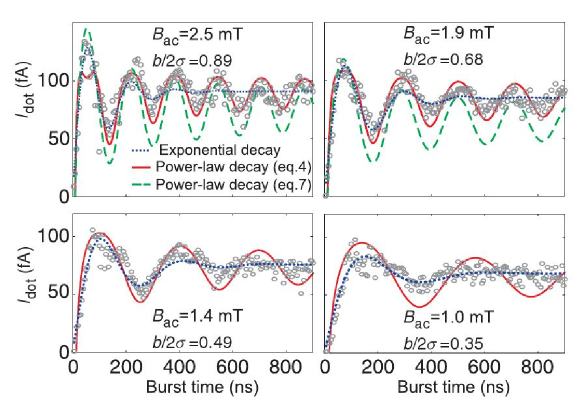
Figure 10: Rabi oscillations for four different driving fields $B_{\mathrm{ac}}$. The gray circles represent the experimental data obtained in the transport measurement as described in the main text. The best fit of eqs. (54) and (55) is represented by solid and dashed lines, respectively. Two fitting parameters were used: the saturation value and the phase shift. The latter turns out to be close to the theoretical value $\pi/4$. See ref. [144] for more information.

These predictions, i.e., both the non-exponential decay and the universal phase shift, have been recently confirmed experimentally [144]. The electron spin state was detected by a transport measurement in a double dot configuration. Electrons are transported through the double quantum dot via transitions from the state with one electron in each dot to the singlet state with two electrons in the right dot, as extensively described in subsubsects. 3.2.2 and 3.5.2. The states with even spin parity (parallel spins) block transport, whereas spins with odd spin parity (antiparallel spins) allow for transport. Given that the system is initialized in an even spin-parity state, the resonant oscillating transverse magnetic field rotates at least one of two electron spins and lifts the blockade. The time evolution of the probability to measure an odd parity state after a time $t$ has been calculated for the following two cases. When both electrons are in resonance with the alternating magnetic field, one finds

$$\begin{split}P_{\mathrm{odd}}^{(2)}(t)=&\frac{1}{2}-2C^{2}-C\sqrt{\frac{2b_{1}}{\sigma^{2}t}}\cos\left(\frac{b_{1}t}{2}+\frac{\pi}{4}\right)\\ &-\frac{b_{1}}{8\sigma^{2}t}\left[1+\cos\left(b_{1}t+\frac{\pi}{4}\right)\right]+o\left(\frac{1}{t^{3/2}}\right).\end{split}$$ (54)

Secondly, when only one electron is on resonance, one obtains

$$P_{\mathrm{odd}}^{(1)}(t)=\frac{1}{2}-C-\sqrt{\frac{b_{1}}{8\sigma^{2}t}}\cos\left(\frac{b_{1}t}{2}+\frac{\pi}{4}\right)+o\left(\frac{1}{t^{3/2}}\right).$$ (55)

The first result eq. (54) is valid for times $t\gtrsim\mathrm{max}\left(1/\sigma,1/b_{1},b_{1}/2\sigma^{2}\right)\sim 20$ ns for a $1.4$ mT nuclear field and $b_{1}\leq 2\sigma$. Note that the $1/t$ term, which becomes important for $b_{1}>\sigma$, oscillates with twice the Rabi frequency. This is the result of the simultaneous rotation of both spins. The term $t^{-1/2}$, which is dominant for $b_{1}<\sigma$, oscillates with the Rabi frequency and stems from the rotation of one spin only. As might be expected from these considerations, $P_{\mathrm{odd}}^{(1)}$ contains exclusively the latter term. The comparison of these theoretical results with the experimental data is presented in fig. 10.

It should be emphasized that the power-law decay and the universal, i.e., independent of all parameters, phase shift $\pi/4$ are obtained with the nuclear field $h_{z}$ being static during a time much longer than the Rabi period. Therefore, the good agreement between the experiment [144] and theory confirms the assumption of a static nuclear bath.

4.2.3 Narrowing of the nuclear state

The evolution of the electron spin governed by eq. (52) depends on the value of the nuclear field since the effective Zeeman splitting is given by $h_{z}^{n}+b$, where $h_{z}\left|n\right>=h_{z}^{n}\left|n\right>$. This means that the resonance condition $b+h_{z}^{n}-\omega=0$ for ESR also depends on the nuclear field. Therefore, a measurement of the electron spin state determines $h_{z}^{n}$ and the related state of the nuclei.

The eigenvalues of the nuclear field in equilibrium obey a Gaussian distribution, as discussed in the previous section. That is, the diagonal elements of the nuclear spin density matrix $\rho_{I}\left(h_{z}^{n},0\right)=\left<n\right|\rho_{I}\left|n\right>=\left(\sqrt{2\pi}\sigma\right)^{-1}\exp\left[-\left(h_{z}^{n}-h_{0}\right)^{2}/2\sigma^{2}\right]$ are Gaussian with mean $h_{0}$ and variance $\sigma$. After the electron spin is initialized in a state $\left|\uparrow\right>$ at time $t=0$, the system evolves under the Hamiltonian $H_{ESR}$ until a measurement of the spin is performed at $t=t_{m}$. Of special interest is the probability to find the electron spin in the orthogonal spin state $\left|\downarrow\right>$ and a given nuclear eigenstate $\left|n\right>$

$$P_{\downarrow}^{n}(t)=\frac{1}{2}\frac{b_{1}^{2}}{b_{1}^{2}+4\delta_{n}^{2}}\left[1-\cos\left(\frac{t\sqrt{b_{1}^{2}+4\delta_{n}^{2}}}{2}\right)\right],$$ (56)

where $b_{1}=g\mu_{B}B_{1}$ as defined before, and $\delta_{n}=b+h_{z}^{n}-\omega$ is the measure of deviation from the resonance condition. On the other hand, the probability to find the electron spin in the state $\left|\downarrow\right>$ with arbitrary configuration of the nuclei is easily obtained by integrating out the nuclear field $P_{\downarrow}(t)=\int dh_{z}^{n}\rho_{I}\left(h_{z}^{n},0\right)P_{\downarrow}^{n}(t)$. The measurement with outcome $\left|\downarrow\right>$ performed on the system results in the collapse of the diagonal part of the nuclear spin density matrix into

$$\rho_{I}\left(h_{z}^{n},0\right)\xrightarrow{\left|\downarrow\right>}\rho_{I}^{(1,\downarrow)}\left(h_{z}^{n},t_{m}\right)=\rho_{I}\left(h_{z}^{n},0\right)\frac{P_{\downarrow}^{n}(t_{m})}{P_{\downarrow}(t_{m})},$$ (57)

according to the basic rules of quantum mechanics. If the measurement has a time resolution smaller than $1/b_{1}$ (i.e., giving time-averaged values), the probability of outcome $\left|\downarrow\right>$ as a function of the nuclear field eigenvalue $h^{z}_{n}$ reads $P_{\downarrow}^{n}=b_{1}^{2}/2(b_{1}^{2}+4\delta_{n}^{2})$. In turn, the nuclear spin density matrix is multiplied by a Lorentzian with width $b_{1}$ and mean $h_{z}^{n}=\omega-b$. As a result, for $b_{1}<\sigma$, the nuclear spin distribution becomes narrowed and prolongation of the electron spin coherence is achieved. Analogously, if the measured outcome is $\left|\uparrow\right>$, the Gaussian nuclear spin distribution is modified as follows:

$$\rho_{I}\left(h_{z}^{n},0\right)\xrightarrow{\left|\uparrow\right>}\rho_{I}^{(1,\uparrow)}\left(h_{z}^{n},t_{m}\right)=\rho_{I}\left(h_{z}^{n},0\right)\frac{1-P_{\downarrow}^{n}(t_{m})}{1-P_{\downarrow}(t_{m})}.$$ (58)

Hence, the probability to match the resonance condition $b+h_{z}^{n}-\omega=0$ is considerably reduced. It has already been proven (cf. subsubsect. 4.2.2) that the nuclear spin evolution is slow enough to allow for multiple measurements of the electron spin (each of them performed after re-initializion to $\left|\uparrow\right>$) over a timescale on which the nuclear spins may be considered static. Repeating the initialization and measurement scheme $M$ times under the assumption of the static nuclear field, we arrive at

$$\rho_{I}\left(h_{z}^{n},0\right)\longrightarrow\rho^{(M,\alpha_{\downarrow})}\left(h_{z}^{n}\right)=\frac{1}{N}\rho_{I}\left(h_{z}^{n},0\right)\left(P_{\downarrow}^{n}\right)^{\alpha_{\downarrow}}\left(1-P_{\downarrow}^{n}\right)^{M-\alpha_{\downarrow}},$$ (59)

where $\alpha_{\downarrow}$ denotes the number of times the state $\left|\downarrow\right>$ was obtained. From the experimental point of view it should be easiest to narrow the nuclear field distribution by performing measurements with $b_{1}\ll\sigma$. Provided that the electron spin was projected to $\left|\downarrow\right>$, the narrowing has been achieved. Otherwise, the additional initialization-measurement cycles should be repeated until the narrowing is observed. The driving frequency should be adjusted after each initialization-measurement cycle to match the resonance condition in order to systematically move towards the narrowed state. Such an adaptive scheme is described in refs. [154] and [63].

4.2.4 Exact solution with a fully polarized nuclear bath

The idea of fully polarizing the nuclear system has attracted considerable attention, since in this special configuration the hyperfine-induced decoherence problem can be overcome. Furthermore, the system of an electron spin confined to a quantum dot with a completely polarized nuclear bath is solvable exactly [155, 156]. Despite the fact that the complete polarization of the nuclear spins is not accessible with current experimental methods (to reduce decoherence by an order of magnitude, polarization of above $99\%$ is required [153], whereas the current world record is about $60\%$ [51]), some schemes to achieve full polarization of the nuclei have been recently proposed. Figure 11 illustrates the temperature range that has to be accessed to directly polarize the nuclei in the presence of the external magnetic field [157]. Cooling to sub-mK temperatures is an experimental challenge which is currently actively pursued. At such low temperatures refs. [158] and [159] predict a phase transition to an ordered nuclear state, even in the absence of the external field. Of crucial importance is in this case the long range nature of the electron-mediated RKKY interaction, which is determined by nonanalytic corrections in the momentum dependence of the electronic spin-susceptibility [159, 160].

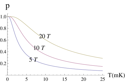
Figure 11: Average nuclear polarization in GaAs ($p=\frac{2}{3N}\sum_{i}\langle I_{i}\rangle$, where $i$ runs over the $N$ nuclei) as a function of temperature at different values of the magnetic field.

Consider a single electron confined to a quantum dot in its ground state. As discussed earlier, coupling of an external field $\mathbf{B}$ to the nuclear spins and direct dipole-dipole interactions among them are negligibly small. Hence, the Hamiltonian can be written as in eq. (44) with $\epsilon=0$ and $H_{dd}=0$. Additionally, we assume that the system is initially in the state $\left|\Psi_{0}\right>=\left|\Downarrow\uparrow\uparrow\cdots\right>=\left|\Downarrow\right>\otimes\left|\uparrow\uparrow\uparrow\cdots\right>$, i.e., the electron spin $|{\Downarrow}\rangle$ is opposite to the fully polarized nuclear bath state $\left|\uparrow\uparrow\uparrow\cdots\right>$. Due to conservation of total angular momentum, the time evolution of the wave function is fully described by $\left|\Psi(t)\right>=\alpha(t)\left|\Psi_{0}\right>+\sum_{k}\beta_{k}(t)\left|\Uparrow\uparrow\uparrow\cdots\downarrow_{k}\cdots\right>$ with the time-dependent coefficients $\alpha(t)$ and $\beta_{k}(t)$ obeying the normalization condition $\left|\alpha(t)\right|^{2}+\sum_{k}\left|\beta_{k}(t)\right|^{2}=1$. The second term in $\left|\Psi(t)\right>$ is a coherent superposition of states with exactly one nuclear spin flipped and thus resembles a magnon excitation.

We will study the correlator $C_{0}(t)=-\left<\Psi_{0}\right|\delta S_{z}(t){S}_{z}\left|\Psi_{0}\right>=\left(1-|\alpha(t)|^{2}\right)/2$, which describes the decay of the electron spin from its initial state $\left|\Downarrow\right>$. Here, $\delta S_{z}(t)=S_{z}(t)-S_{z}$, where $S_{z}(t)$ is the Heisenberg representation of $S_{z}$. Inserting $\left|\Psi(t)\right>$ into the Schrödinger equation, we obtain a set of coupled differential equations of the form

$$2i\frac{d\alpha(t)}{dt}=-A\alpha(t)/2+\sum_{k}A_{k}\beta_{k}(t)-b\alpha(t),$$ (60)

$$2i\frac{d\beta_{l}(t)}{dt}=\left(A/2-A_{l}\right)\beta_{l}(t)+A_{l}\alpha(t)+b\beta_{l}(t),$$ (61)

with $A=\sum_{k}A_{k}$ and $b=g\mu_{B}B$. These equations can be solved in the usual way by performing a Laplace transform $\alpha(u)=\int_{0}^{\infty}dt\alpha(t)e^{-ut}$. One obtains

$$\alpha(u)=i\frac{\alpha(0)}{D(u)}+\frac{i}{2D(u)}\sum_{k}\frac{A_{k}\beta_{k}(0)}{iu-(A+2b)/4+A_{k}/2},$$ (62)

where

$$D(u)=iu+\frac{A+2b}{4}-\frac{1}{4}\sum_{k}\frac{A_{k}^{2}}{iu-(A+2b)/4+A_{k}/2}.$$ (63)

Defining $iu=i\omega+(A+2b)/4$, using the initial conditions $\alpha(0)=1$ and $\beta_{k}(0)=0$, and replacing the sum over $k$ by an integral, i.e.,

$$\sum_{k}\frac{A_{k}^{2}}{i\omega+A_{k}/2}=2\left[A-2\pi iN\omega\int dz\ln\left(1-\frac{iA\chi_{0}^{2}(z)}{2\pi N\omega}\right)\right],$$ (64)

where $\chi_{0}(z)$ is the normalized transverse wave function defined through the envelope wave function $|\Psi(r,z)|^{2}=\exp(-r^{2}/a^{2})\chi_{0}^{2}(z)/(\pi a^{2}a_{z})$, where $a$ and $a_{z}$ are dot’s dimensions in the lateral and transverse direction, respectively, one arrives at the following expression for $\alpha(t)$ (required to calculate the correlator $C_{0}(t)$)

$$\alpha(t)=\frac{e^{-iA^{\prime}t/4}}{2\pi}\int_{\gamma-i\infty}^{\gamma+i\infty}d\omega\frac{e^{i\omega t}}{i\omega+b+\pi Ni\omega\int dz\ln\left(1-\frac{iA\chi_{0}^{2}(z)}{2\pi N\omega}\right)}.$$ (65)

Here, $A^{\prime}=A+2b$, and $z$ is dimensionless in units of $a_{z}$. The integration contour is a vertical line in the complex $\omega$ plane such that all singularities lie to its left. There are two types of singularities: two branch points $\omega=0$ and $\omega_{0}=iA\chi_{0}^{2}(0)/2\pi N$, and first order poles which lie on the imaginary axis ($\omega=i\upsilon$). For $b>0$ there is one pole, while for $b<0$ there are two poles; for $b=0$ there is one pole at $\omega_{1}\approx iA/2+iA\int dz\chi_{0}^{4}(z)/4\pi N$. The contribution from the branch cut between $\omega=0$ and $\omega=\omega_{0}$ is

$$\tilde{\alpha}(t)=\frac{e^{-iA^{\prime}t/4}}{\pi N}\int_{0}^{1}d\kappa\frac{2z_{0}\kappa e^{i\tau^{\prime}\kappa}}{\left|\kappa\int dz\left|\chi_{0}^{2}(z)/\chi_{0}^{2}(0)\kappa-1\right|+\kappa/\pi N-2b/A\chi_{0}^{2}(0)\right|^{2}+\left(2\pi z_{0}\right)^{2}\kappa^{2}},$$ (66)

where $\tau^{\prime}=\tau\chi_{0}^{2}(0)$ with $\tau=At/2\pi N$, and $z_{0}=z_{0}(\kappa)$ is defined through $\chi_{0}^{2}(z_{0})=\chi_{0}^{2}(0)\kappa$. $N=n_{0}a_{z}a^{2}$ is a number of nuclear spins of density $n_{0}$ and we have introduced the dimensionless variable $\kappa=\omega/\omega_{0}\leq 1$.

The physical picture is the following. At time $t=0$ the system has some energy corresponding to the pole. It then starts oscillating back and forth, while each time visiting different frequencies within the branch cut. This corresponds to the flip-flop processes with the nuclei located at different sites. The contribution from the branch cut therefore describes the electron spin decoherence. At time $\tau\sim 1$ (where the decay mainly takes place) the decoherence is due to the interaction with the nuclei located at distances of order of the dot radius where the derivative of the coupling constant is maximal. For longer times, $\tau\gg 1$, the asymptotic behavior is determined either by the interaction with the nuclei located far from the dot or near the dot center depending on the Zeeman field value.

First, consider the limit of large Zeeman field ($b\gg A$) and large times ($\tau\gg 1$). The main contribution to the integral comes from $\kappa\rightarrow 1$, i.e., by the interaction with the nuclei located near the dot center. The asymptotic behavior of $\tilde{\alpha}(t)$ is

$$\tilde{\alpha}(\tau\gg 1)=\frac{e^{-iA^{\prime}t/4}e^{i\tau^{\prime}}}{\pi N}\frac{\chi_{0}^{2}(0)}{\sqrt{\left(\chi_{0}^{2}\right)^{\prime\prime}}}\frac{A^{2}}{b^{2}}\frac{(1-i)\sqrt{\pi}}{4i\tau^{3/2}}\propto\frac{1}{N}\left(\frac{A}{b}\right)^{2}.$$ (67)

Here, $(\chi_{0}^{2})^{\prime\prime}$ denotes the second derivative of $\chi_{0}^{2}$ evaluated at $z=0$. Remember that the correlation function is given by $C_{0}(t)=\left(1-|\alpha(t)|^{2}\right)/2$ and that $\alpha(t)$ contains, besides the branch cut contribution $\tilde{\alpha}(t)$ (which is a decaying function of time), an oscillating term due to the pole contribution. Therefore, the leading term in the full correlator for $\tau\gg 1$ is a constant, given by the square of the modulus of the pole contribution. The next higher correction is the product of the pole contribution and $\tilde{\alpha}(t)$ as stated above.

Secondly, for the magnetic field turned off ($b=0$) the asymptotic behavior of the integrand in eq. (66) for $\tau\gg 1$ is determined by $\kappa\ll 1$. Taking for instance $\chi_{0}^{2}(z)/\chi_{0}^{2}(0)=e^{-z^{2}}$, we find

$$\tilde{\alpha}(\tau\gg 1)\propto 1/\ln^{\frac{3}{2}}\tau.$$ (68)

This result is non-universal. It depends on the form of the electron wave function at distances larger than the dot size, since the decoherence is due to the interaction with the nuclei located far from the dot. The disturbance of the nuclear spins propagates from the center of the dot outwards.

To summarize this part, we have shown that the decaying part of the correlator $C_{0}(t)$ is strongly affected by the magnetic field strength. However, the characteristic time scale for the onset of the non-exponential decay is the same for all cases and is given by $(A/N)^{-1}$. For GaAs quantum dots, this is in the range of microseconds.

4.2.5 Time evolution with arbitrary nuclear polarization

In the previous section we discussed the exactly solvable case of an electron spin coupled to a fully polarized nuclear bath. However, for an initial nuclear spin configuration which is not completely polarized, no exact solution exists and standard time-dependent perturbation theory fails [155, 156]. In this section, we review a systematic approach to the electron spin dynamics in the presence of the Fermi contact hyperfine interaction eq. (45). This theory is valid in the limit of high magnetic fields and for arbitrary spin polarization and nuclear spin $I$ ($I=3/2$ in GaAs). Furthermore, the initial state of the system is $\rho(0)=\rho_{S}(0)\otimes\rho_{I}(0)$ and it is assumed that $\rho_{I}(0)=|n\rangle\langle n|$, where $|n\rangle$ is an eigenstate of $h_{z}$. In practice, this is not usually the case and an appropriate ‘narrowing’ procedure as the one described in subsubsect. 4.2.3 has to be applied. Throughout this section and in the next one we also assume isotropic hyperfine couplings (in $d$ dimensions)

$$A_{k}=A_{0}\exp\left[-\left(\frac{r_{k}}{l_{0}}\right)^{q}\right],$$ (69)

where $r_{k}$ is the radial coordinate of the $k$-th nuclear site. Note that $\sum_{k}A_{k}=A$, and therefore $A_{0}\sim A/N$, where $N$ is defined as the number of nuclei within the radius $l_{0}$ and $A\sim 90~{}\mu{\rm eV}$ in GaAs. In the following, we choose the unit of energy such that $A_{0}=2$.

We follow ref. [153] and start from the generalized master equations describing the exact dynamics of the reduced electron spin polarization

$$\langle\dot{S}_{z}\rangle_{t} =N_{z}(t)-i\int_{0}^{t}dt^{\prime}\Sigma_{zz}(t-t^{\prime})\langle S_{z}\rangle_{t^{\prime}},$$ (70)

$$\langle\dot{S}_{+}\rangle_{t} =i\omega_{n}\langle S_{+}\rangle_{t}-i\int_{0}^{t}dt^{\prime}\Sigma_{++}(t-t^{\prime})\langle S_{+}\rangle_{t^{\prime}},$$ (71)

where $\omega_{n}=b^{\prime}+\langle n|h_{z}|n\rangle$ and $S_{\pm}=S_{x}\pm iS_{y}$. It is also useful to introduce the reduced self-energy superoperator, which acts on a generic operator $O$ as follows [153]

$$\hat{\Sigma}_{S}(t)O=-i\mathrm{Tr}_{I}\left\{\hat{L}e^{-i\hat{Q}\hat{L}t}\hat{L}_{V}[\rho_{I}(0)O]\right\},$$ (72)

where $\hat{L}=\hat{L}_{0}+\hat{L}_{V}$ is the full Liouvillian superoperator, defined by $\hat{L}_{0}O=[H_{0},O]$ and $\hat{L}_{V}O=[V,O]$, the superoperator $\hat{Q}$ is defined by $\hat{Q}O=O-\rho_{I}(0)\mathrm{Tr}_{I}O$, and $\mathrm{Tr}_{I}$ is the partial trace over the nuclear degrees of freedom. By using eq. (72) above, we can write the kernel of eq. (71) as $\Sigma_{++}(t)=\mathrm{Tr}_{S}[S_{-}\hat{\Sigma}_{S}(t)S_{+}]$, where $\mathrm{Tr}_{S}$ is the partial trace over the electron spin. We also define $\Sigma_{\mu\nu}(t)=\mathrm{Tr}_{S}[\rho_{\mu}\hat{\Sigma}_{S}(t)\rho_{\nu}]$ where $\mu,\nu=\uparrow,\downarrow$ and $\rho_{\uparrow(\downarrow)}=(1\pm\sigma_{z})/2$. In terms of these quantities, the kernel of eq. (70) is given by $\Sigma_{zz}(t)=\Sigma_{\uparrow\uparrow}(t)-\Sigma_{\uparrow\downarrow}(t)$. Finally, the inhomogeneous term of eq. (70) is most simply defined in terms of its Laplace transform $f(s)=\int_{0}^{\infty}dtf(t)e^{-st}$, which gives $N_{z}(s)=(2is)^{-1}\left[\Sigma_{\uparrow\uparrow}(s)+\Sigma_{\uparrow\downarrow}(s)\right]$.

Solutions to eqs. (70) and (71) cannot be obtained exactly and, to proceed further, an expansion in powers of the flip-flop term $V$ (see eq. (45)) is performed. The self-energy superoperator (72) can be expressed as a series in terms of $\hat{L}_{V}$, where only even powers appear, i.e., $\Sigma_{S}(t)=\Sigma^{(2)}_{S}(t)+\Sigma^{(4)}_{S}(t)+\ldots\,\,$. At order $2(k+1)$, the self-energy contribution is suppressed at least by a factor $\Delta^{k}$, where $\Delta=N/\omega_{n}$ becomes small at large values of the external magnetic field. Therefore, the Born approximation $\Sigma_{S}(t)=\Sigma^{(2)}_{S}(t)$ is justified in this limit. The time evolution can be determined from the Laplace transforms of eqs. (70) and (71), which involve the following lowest-order self-energies

$$\Sigma_{\uparrow\uparrow}^{(2)}(s) =-iNc_{+}\left[I_{+}(s-i\omega_{n})+I_{-}(s+i\omega_{n})\right],$$ (73)

$$\Sigma_{\uparrow\downarrow}^{(2)}(s) =iNc_{-}\left[I_{-}(s-i\omega_{n})+I_{+}(s+i\omega_{n})\right],$$ (74)

$$\Sigma_{++}^{(2)}(s) =-iN\left[c_{-}I_{+}(s)+c_{+}I_{-}(s)\right],$$ (75)

where $c_{\pm}=I(I+1)-\left<\right<m(m\pm 1)\left>\right>$ and $\left<\right<F(m)\left>\right>=\sum_{m=-I}^{I}P(m)F(m)$. Here, $P(m)$ is the probability to find a nuclear spin with $z$-projection $m$ and $F(m)$ is an arbitrary function (for example $\left<\right<m\left>\right>=pI$ gives the polarization $p$ of the initial state). The explicit expression of $I_{\pm}(s)$ reads

$$I_{\pm}(s)=\frac{1}{4N}\sum_{k}\frac{A_{k}^{2}}{s\mp iA_{k}/2}=\frac{d}{m}\int_{0}^{1}dx\frac{x|\ln x|^{\nu}}{s\mp ix},$$ (76)

where $\nu=d/q-1$ and we performed the continuum limit using eq. (69). Two examples obtained inverting eq. (76) are plotted in fig. 12 as functions of time. Note that $t$ is in units of $2/A_{0}$, which corresponds to a timescale of order $N/A\sim 1~{}\mu{s}$.

We describe next the case $\Delta\ll 1$, in which the solution has a simple form in terms of the small parameter $\delta=N/\omega_{n}^{2}$. The longitudinal component is given by $\langle S_{z}\rangle_{t}=\langle S_{z}\rangle_{\infty}+\sigma_{z}^{\rm dec}(t)$, where

$$\langle S_{z}\rangle_{\infty}=[1-2\,\delta\,I_{0}(c_{+}+c_{-})]\langle S_{z}\rangle_{0}+2\,pI\,\delta I_{0},$$ (77)

$$\sigma_{z}^{\rm dec}(t)=2\,\delta\,{\rm Re}\left[\left(C_{+}I_{-}(t)+C_{-}I_{+}(t)\right)e^{-i\omega_{n}t}\right].$$ (78)

Here, $I_{0}=I_{\pm}(t=0)$, $c_{\pm}$ were defined before, and $C_{\pm}=c_{\pm}(\langle S_{z}\rangle_{0}\pm\frac{1}{2})$. The transverse solution is $\langle S_{+}\rangle_{t}=\sigma_{+}^{\rm osc}(t)+\sigma_{+}^{\rm dec}(t)$, where

$$\sigma_{+}^{\rm osc}(t)=[1-\delta\,I_{0}(c_{+}+c_{-})]\langle S_{+}\rangle_{0}e^{i\omega_{n}t},$$ (79)

$$\sigma_{+}^{\rm dec}(t)=\delta\left[c_{+}I_{-}(t)+c_{-}I_{+}(t)\right]\langle S_{+}\rangle_{0}.$$ (80)

In both cases, the solution is expressed as a sum of a term which is constant in absolute value ($\langle S_{z}\rangle_{\infty}$ and $\sigma_{+}^{\rm osc}(t)$ respectively), and a decaying part ($\sigma_{z}^{\rm dec}(t)$ and $\sigma_{+}^{\rm dec}(t)$ respectively). The former is almost equal to the initial polarization, $\langle S_{z}\rangle_{0}$ or $\langle S_{+}\rangle_{0}$, except a correction of order $\delta$. Reintroducing dimensional units (i.e., multiplying by $A_{0}^{2}/4$), one obtains that the fraction of polarization which decays is $\delta\sim A^{2}/\omega_{n}^{2}N$. The time dependence of this decaying contribution is determined by the $I_{\pm}(t)$ functions. As illustrated in fig. 12, the $I_{\pm}(t)$ can have a very different form, depending on the ratio $d/q$. In particular

$$I_{\pm}(t\gg 1)\propto\frac{e^{\pm it}}{t^{d/q}}\qquad\qquad{\rm for}~{}\frac{d}{q}<2,$$ (81)

$$I_{\pm}(t\gg 1)\propto\frac{(\ln t)^{\frac{d}{q}-1}}{t^{2}}\qquad{\rm for}~{}\frac{d}{q}\geq 2,$$ (82)

where the first expression is determined by the nuclei close to the origin, and the second one from distant nuclei with a small coupling $A_{k}$. These two asymptotic forms are relevant in different physical situations, e.g., the first one for $s$-type hydrogenic functions of Si impurities ($d=3$ and $q=1$) and the second for a parabolic quantum dot in two dimensions ($q=d=2$). Note that in eq. (81) the decay has an oscillatory character, differently from eq. (82).

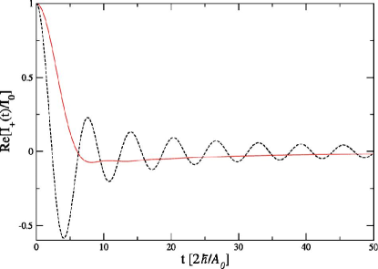
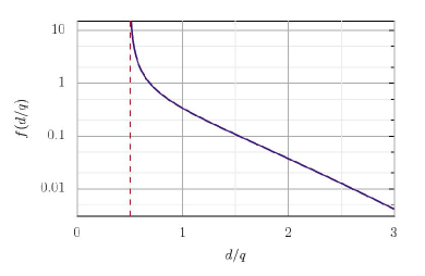
Figure 12: Left panel: Plot of ${\rm Re}[I_{+}(t)/I_{+}(0)]$, as obtained from eq. (76). The solid line was calculated with $d=3$ and $m=1$, which is appropriate for a hydrogen $s$-type envelope wave function. The dashed curve refers to a two-dimensional Gaussian envelope wave function ($d=m=2$). The asymptotic behaviors in the two cases are given in eqs. (82) and (81) respectively. Right panel: Geometrical factor $f(d/q)$ defined by eq. (87), with $d$ being the dimensionality and $q$ is related to the shape of the ground-state wave function (see eq. (69)).

Within the second-order Born approximation scheme discussed here, the time evolution at generic values of the expansion parameter $\Delta<1$ offers a rich scenario, including terms with exponential decay, non-exponential decay, and undamped oscillations. The same method also reproduces the exact solution of the previous section, at $p=1$, and can be extended to higher order in $\hat{L}_{V}$. We refer to ref. [153] for the detailed treatment of these topics. As a final comment we note that the electron spin dynamics, as described at this level of approximation, is non-Markovian. For large times the electron spin polarization does not display an exponential decay but is constant in magnitude. The interesting part of the time dependence is given by the small decaying functions $\sigma_{z}^{\rm dec}(t)$ and $\sigma_{+}^{\rm dec}(t)$, which also have a non-exponential charater, see eqs. (81) and (82). This picture is reexamined in the next section, where a different result (i.e., Markovian decay) is found at very large time scales ($T_{2}\sim\omega_{n}^{2}N/A^{3}$, see also fig. 13).

4.2.6 Markovian dynamics

At large magnetic fields, it is in principle possible to carry on the perturbative treatment of the previous section in terms of $V$ to an arbitrary accuracy. Higher order corrections to the self-energy are multiplied by a small factor $\Delta$ and are expected to be small. However, it will become clear in the following that these initially small perturbative corrections can grow with time and become significant. Therefore, we reexamine the problem of the previous section (i.e., the time evolution of the spin polarization if the initial state $|n\rangle$ of the nuclear bath is an eigenstate of $h_{z}$) with special attention to the time evolution at large time scales. We focus on the transverse component, generally described by eq. (71). Full decay of this polarization component at large times, of order $\omega_{n}N/A^{2}\gg N/A$, is found in ref. [161] and an asymptotic dependence $\propto 1/t^{2}$ is derived in Ref [162]. It is therefore necessary to improve the treatment yielding eqs. (79) and (80) to describe the full decay of the transverse polarization. We outline here a different method of solution, which in fact predicts a Markovian spin decay at large times [163].

As a first step, consider the following second order effective Hamiltonian derived from a Schrieffer-Wolff transformation of eq. (44)

$$H_{\mathrm{eff}}=\left(b+h_{z}+\frac{1}{2}\sum_{k\neq l}\frac{A_{k}A_{l}}{\omega}I_{k}^{-}I_{l}^{+}\right)S_{z}+b\sum_{k}\gamma_{k}I_{k}^{z},$$ (83)

where $\omega=b+h_{z}$ and $I_{k}^{+}$ ($I_{k}^{-}$) is the raising (lowering) ladder operator for the nuclear spins at site $k$. Differently from eq. (44), a site-dependent nuclear $g$-factor $g_{I_{k}}$ is taken into account, such that $\gamma_{k}=g_{I_{k}}\mu_{N}/g\mu_{B}$, and the term $H_{dd}$ is omitted. The Schrieffer-Wolff transformation was performed assuming that corrections to the diagonal part of $H_{\mathrm{eff}}$ of order of $\sim A^{2}/Nb$ can be neglected, but corrections of the same order to the non-diagonal part should be retained. This is justified by the fact that the bath correlation time $\tau_{c}\sim N/A\ll Nb/A^{2}$ is small compared to the time scale on which the diagonal corrections become relevant for $b\gg A$.

In this effective Hamiltonian, the perturbing term is $V_{\rm eff}=XS_{z}$, where $X$ is given by $X=1/2\sum_{k\neq l}A_{k}A_{l}I_{k}^{-}I_{l}^{+}/\omega$. We can now proceed as in the previous section, and approximate the memory kernel $\Sigma_{++}(t)$ of eq. (71) to lowest order in $V_{\rm eff}$. However, the result obtained in this case is more accurate: the second order Born approximation in $V_{\rm eff}$, applied to (83), retains contributions up to fourth order in the hyperfine couplings $A_{k}$. Differently from the previous section, the Markov approximation can be applied in this case, and leads to a non-vanishing decay. The decoherence rate

$$\frac{1}{T_{2}}=\mathrm{Re}\int_{0}^{\infty}dte^{-i\Delta\omega t}\left<X(t)X(0)\right>$$ (84)

is given in terms of the non-diagonal part dynamics $X(t)=e^{-i\omega t}Xe^{i\omega t}$. The expectation value is taken with respect to the initial ‘narrowed’ nuclear spin state and $\Delta\omega$ is a shift of the precession frequency (i.e., $\langle S_{+}\rangle_{t}=\frac{x_{t}}{2}e^{i(\omega_{n}+\Delta\omega)t}$, where $x_{t}$ is a slowly varying envelope) which has to be determined self-consistently, see ref. [163]. Provided that the initial nuclear spin polarization is smooth on the scale of the electron wave function, the matrix elements of operators such as $I_{k}^{\pm}I_{k}^{\mp}$ can be replaced by their average values and the correlator $\left<X(t)X(0)\right>$ takes the form

$$\left<X(t)X(0)\right>=\frac{c_{+}c_{-}}{4\omega_{n}^{2}}\sum_{k\neq l}A_{k}^{2}A_{l}^{2}e^{-i(A_{k}-A_{l})t},$$ (85)

where $c_{\pm}$ are as in the previous section and $\omega_{n}=\langle n|\omega|n\rangle$ . We consider now an initially uniform unpolarized state with equal populations of all nuclear Zeeman levels. This means that $\left<\right<m\left>\right>=0$ and $\left<\right<m^{2}\left>\right>=I(I+1)/3$, while $\omega_{n}=b$. The final result takes the particularly simple form

$$\frac{1}{T_{2}}=\pi\left(\frac{I(I+1)A}{3b}\right)^{2}f\left(\frac{d}{q}\right)\frac{A}{N},$$ (86)

where

$$f\left(\frac{d}{q}\right)=\frac{q}{d}\left(\frac{1}{3}\right)^{2\frac{d}{q}-1}\frac{\Gamma(2d/q-1)}{(\Gamma(d/q))^{3}},$$ (87)

which is valid for any dimensionality provided that $d/q>1/2$. The geometrical factor dependence is shown in the right plot of fig. 12. In 3D it may describe a donor impurity, in 2D a lateral gated quantum dot, while in 1D a nanotube or a nanowire. Note that for $q/d=2$ the decoherence rate diverges so that the decoherence time tends to zero, which signals the failure of the Makov approximation. Furthermore, $1/T_{2}\propto I^{4}$ depends strongly on the nuclear spin so that systems with large magnetic moment like In (with $I=9/2$) exhibit faster decay than, for instance, GaAs (with $I=3/2$). Finally, the validity condition for the Markov approximation, $T_{2}>\tau_{c}\sim N/A$ is satisfied if $A/b<1$, and coincides with the requirement for the Born approximation.

In heteronuclear systems the decoherence time is given by the sum of decoherence rates weighted by the natural abundance of each isotope $\nu_{i}$ squared, i.e., $1/T_{2}=\sum_{i}\nu_{i}^{2}\Gamma_{i}$, if interspecies flip-flops are neglected. The quadratic dependence on isotopic concentration is particularly striking. In spite of the fact that all isotopes in GaAs have the same nuclear spin and nominally the same hyperfine coupling constant, the decay is dominated by intraspecies flip-flops between As spins. This effect may both explain why only Ga spins have been seen to contribute to coherent effects in transport experiments through (In/Ga)As quantum dots [145] and why polarization seems to be transferred more efficiently from electron to As – rather than Ga – in GaAs quantum dots [164].

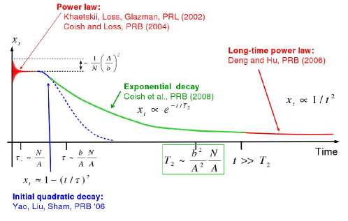
Figure 13: Schematic representation of the decay of the transverse polarization. The different regimes are discussed in subsubsects. 4.2.5 and 4.2.6.

Finally, taking into account the discussion of the present section, we summarize in fig. 13 the functional dependence of the transverse spin polarization. There, four regimes are schematically depicted : (i) If $t<\tau_{c}\sim N/A$, the power law decay discussed in the previous section applies [155, 156, 153]. (ii) If $\tau_{c}\ll t\ll\tau\sim bN/A^{2}$, a quadratic correction $\propto-(t/\tau)^{2}$ is obtained in ref. [161]. (iii) If $\tau<t\ll T_{2}\sim(b/A)^{2}(N/A)$, the exponential decay $\propto e^{-t/T_{2}}$ discussed in this section is valid [163]. (iv) If $t\gg T_{2}$, the long-time power law decay is $\propto 1/t^{2}$ [162].

The Schrieffer-Wolff transformation

The Schrieffer-Wolff transformation is a very useful method to treat the coupling of external orbital perturbations to the spin states in the presence of spin-orbit interaction. It is applied to the theoretical treatment of EDSR in quantum dots (see Section 3.4.1) and spin relaxation due to phonons and other charge fluctuations (see Section 4). We give here some additional details on the subject (see also ref. [131]).

The Hamiltonian treated here is similar to eq. (25) and (34). More specifically, we consider $H=H_{d}+H_{Z}+H_{SO}+V(t)$, where the unperturbed dot Hamiltonian is $H_{d}={\bf p}^{2}/2m^{*}+U({\bf r})$ as before (the eigenstates are $|n,\pm\rangle=\psi_{n}({\bf r})|\pm\rangle$, with energy $\epsilon_{n}$). The only difference is that $V(t)$ refers here to a general orbital perturbation, whereas in eq. (25) and eq. (34) $V(t)$ specifically is the external ac electric field and the electron-phonon coupling, respectively.

Consider now a unitary transformation of $H$ of the form

$$\tilde{H}=e^{S}He^{-S}\simeq H_{d}+H_{Z}+V(t)+[S,V(t)]+\ldots$$ (88)

where $S$ satisfies $[H_{d}+H_{Z},S]=H_{SO}$, such that the spin-orbit perturbation $H_{SO}$ does not appear in $\tilde{H}$. The transformed Hamiltonian $\tilde{H}$ is accurate to first order in the spin-orbit coupling, which determines the last term $[S,V(t)]$. The solution for $S$ can be formally written in terms of the Liouvillian superoperators $\hat{L}_{d(Z)}$ defined by $\hat{L}_{d(Z)}A=[H_{d(Z)},A]$, where $A$ is a generic electron operator. Note that the spin-orbit coupling in the form of eq. (26) can be written as $H_{SO}=i[H_{d},\boldsymbol{\sigma}\cdot\boldsymbol{\xi}]=i\hat{L}_{d}\boldsymbol{\sigma}\cdot\boldsymbol{\xi}$, where $\boldsymbol{\xi}=(y/\lambda_{-},x/\lambda_{+},0)$ and $S$ satisfies

$$(\hat{L}_{d}+\hat{L}_{Z})S=i\hat{L}_{d}\boldsymbol{\sigma}\cdot\boldsymbol{\xi}.$$ (89)

To every order in $\hat{L}_{Z}$, eq. (89) is solved by

$$S=(1-\hat{P})\sum_{n=0}^{\infty}(-\hat{L}_{d}^{-1}\hat{L}_{Z})^{n}~{}i\boldsymbol{\sigma}\cdot\boldsymbol{\xi},$$ (90)

where $\hat{L}_{d}^{-1}=-i\int_{0}^{\infty}e^{i(\hat{L}_{d}+i\eta)t}{\rm d}t$, with $\eta=0^{+}$, and $\hat{P}$ is such that $\langle n\sigma|\hat{P}A|n^{\prime}\sigma^{\prime}\rangle=\langle n\sigma|A|n^{\prime}\sigma^{\prime}\rangle$ if $\epsilon_{n}=\epsilon_{n^{\prime}}$ and $\langle n\sigma|\hat{P}A|n^{\prime}\sigma^{\prime}\rangle=0$ otherwise. Therefore, $\hat{P}A$ commutes with $H_{d}$ and $\hat{L}_{d}\hat{P}=0$. Furthermore, $\hat{L}_{d}$ and $\hat{L}_{Z}$ commute (since $H_{d}$ and $H_{Z}$ do) and $\hat{L}_{d}^{-1}$ and $\hat{P}$ commute with them as well, following directly from their definitions. By making use of these properties, one can verify that (89) is satisfied by (90).

We can now calculate the effective potential $[S,V(t)]$. The first non-vanishing contribution to the commutator is obtained to first order in $\hat{L}_{Z}$ and can be written in the following form

$$[S,V(t)]=[g\mu_{B}\boldsymbol{\sigma}\cdot({\bf B}\times(1-\hat{P})\hat{L}_{d}^{-1}\boldsymbol{\xi}),V(t)]+\ldots.$$ (91)

Finally, we derive an effective spin Hamiltonian by calculating the expectation value $\langle\psi_{0}({\bf r})|\tilde{H}|\psi_{0}({\bf r})\rangle$ with respect to the ground state orbital wave function of $H_{d}$. Neglecting spin-independent terms we obtain

$$H_{\rm eff}=\frac{g\mu_{B}}{2}{\bf B}\cdot\boldsymbol{\sigma}+g\mu_{B}({\bf B}\times\boldsymbol{\Omega}(t))\cdot\boldsymbol{\sigma},$$ (92)

where the first term is the usual Zeeman coupling and an additional effective magnetic field is produced by $V(t)$ through $\boldsymbol{\Omega}(t)$, which is defined by

$$\boldsymbol{\Omega}(t)=\langle\psi_{0}({\bf r})|[(1-\hat{P})\hat{L}_{d}^{-1}\boldsymbol{\xi},V(t)]|\psi_{0}({\bf r})\rangle.$$ (93)

References

- [1] \NAMEDeutsch D., \INProc. R. Soc. London, Ser. A400198597.
- [2] \NAMEFeynman R. P., \INInt. J. Theor. Phys.211982467.
- [3] \NAMEFeynman R. P., \INFound. Phys.161986507.
- [4] \NAMEAspect A., Grangier P. \atqueRoger G., \INPhys. Rev. Lett.49198291.
- [5] \NAMEEinstein A., Podolsky B. \atqueRosen N., \INPhys. Rev.471935777.
- [6] \NAMESchrödinger E., \INNaturwissenschaften231935823.
- [7] \NAMELoss D. \atqueDiVincenzo D. P., \INPhys. Rev. A571998120.
- [8] \NAMEBulaev D. V., Trauzettel B. \atqueLoss D., \INPhys. Rev. B772008235301.
- [9] \NAMETrif M., Golovach V. N. \atqueLoss D., \INPhys.Rev. B772008045434.
- [10] \NAMELeuenberger M. N. \atqueLoss D., \INNature4102001789.
- [11] \NAMEMeier F., Levy J. \atqueLoss D., \INPhys. Rev. Lett.902003047901.
- [12] \NAMELehmann J., Gaita-Arin̄o A., Coronado E. \atqueLoss D., \INNat. Nanotechnol.22007312.
- [13] \NAMETrif M., Troiani F., Stepanenko D. \atqueLoss D., \INPhys. Rev. Lett.1012008217201.
- [14] \NAMETrauzettel B., Bulaev D. V., Loss D. \atqueBurkard G., \INNat. Phys.32007192.
- [15] \NAMEChildress L., Gurudev Dutt M. V., Taylor J. M., Zibrov A. S., Jelezko F., Wrachtrup J., Hemmer P. R. \atqueLukin M. D., \INScience3142006281.
- [16] \NAMEAwschalom D. D., Epstein R. \atqueHanson R., \INSci. Am.297200784.
- [17] \NAMEDutt M. V. G., Childress L., Jiang L., Togan E., Maze J., Jelezko F., Zibrov A. S., Hemmer P. R. \atqueLukin M. D., \INScience31620071312.
- [18] \NAMENeumann P., Mizuochi N., Rempp F., Hemmer P., Watanabe H., Yamasaki S., Jacques V., Gaebel T., Jelezko F. \atqueWrachtrup J., \INScience32020081326.
- [19] \NAMEDiVincenzo, \INFortschr. Phys.482000771.
- [20] \NAMEChurch J., \INAm. J. Math.581936435.
- [21] \NAMETuring A. M., \INProc. Lond. math. Soc. Ser. 24421936230.
- [22] \NAMEPapadimitriou C. M., \TITLEComputational Complexity (Addison-Wesley, Reading, Massachusetts) 1994.
- [23] \NAMEChernoff H., \INAnn. Math. Statist.231952493.
- [24] \NAMENielsen M. A. \atqueChuang I. L., \TITLEQuantum Computation and Quantum Information (Cambridge University Press, New York) 2000.
- [25] \NAMEWootters W. K. \atqueZurek W. H., \INNature2991982802.
- [26] \NAMEBarenco A., Bennett C. H., Cleve R., DiVincenzo D. P., Margolus N., Shor P., Sleator T., Smolin J. A. \atqueWeinfurter H., \INPhys. Rev. A5219953457.
- [27] \NAMEBernstein E. \atqueVazirani U., \INSiam Journal on Computing2619971411.
- [28] \NAMECleve R., arXiv:quant-ph/9906111 (1999).
- [29] \NAMEDeutsch D. \atqueJozsa R., \INProc. R. Soc. London, Ser. A4391992553.
- [30] \NAMECleve R., Ekert A., Macchiavello C. \atqueMosca M., \INProc. R. Soc. London, Ser. A4541998339.
- [31] \NAMEGrover L. K., \TITLEA fast quantum mechanical algorithm for database search, in \TITLEProceedings, 28th Annual ACM Symposium on the Theory of Computing 1996, p. 212 (arXiv:quant-ph/9605043).
- [32] \NAMEShor P., \INSIAM Journal on Computing2619971484.
- [33] \NAMERivest R., Shamir A. \atqueAdleman L., \INCommunications of the ACM211978120.
- [34] \NAMEKitaev A., Shen A. \atqueVyalyi M. N., \TITLEClassical and Quantum Computation (American Mathematical Society) 2002.
- [35] \NAMEAharonov D. \atqueNaveh T., arXiv:quant-ph/0210077 (2002).
- [36] \NAMEKempe J., Kitaev A. \atqueRegev O., \INSIAM J. Comput.3520061070.
- [37] \NAMEPreskill J., \INProc. R. Soc. London, Ser. A4541998385.
- [38] \NAMEAliferis P. \atquePreskill J., arXiv:0710.1301 (2007).
- [39] \NAMEGottesman D., \INJ. Mod. Optics472000333.
- [40] \NAMEHanson R., Kouwenhoven L. P., Petta J. R., Tarucha S. \atqueVandersypen L. M. K., \INRev. Mod. Phys.7920071217.
- [41] \NAMECoish W. A. \atqueLoss D., in \TITLEHandbook of Magnetism and Advanced Materials, edited by \NAMEKronmüler H. \atqueParkin S., Vol. 5 (Wiley, New York) 2007, p. 2895, (arXiv:cond-mat/0606550).
- [42] \NAMEFiederling R., Keim M., Reuscher G., Ossau W., Schmidt G., Waag A. \atqueMolenkamp L. W., \INNature4021999787.
- [43] \NAMEOhno Y., Young D. K., Beschoten B., Matsukara F., Ohno H. \atqueAwschalom D. D., \INNature4021999790.
- [44] \NAMEPrinz G. \atqueHathaway K., \INPhysics Today48199524.
- [45] \NAMEPrinz G. A., \INScience28219981660.
- [46] \NAMEDiVincenzo D. P., \INJour. Appl. Phys.8519994785.
- [47] \NAMERecher P., Sukhorukov E. V. \atqueLoss D., \INPhys. Rev. Lett.8520001962.
- [48] \NAMECortez S., Krebs O., Laurent S., Senes M., Marie X., Voisin P., Ferreira R., Bastard G., G’erard J.-M. \atqueAmad T., \INPhys. Rev. Lett.892002207401.
- [49] \NAMEShabaev A., Efros A., Gammon D. \atqueMerkulov I. A., \INPhys. Rev. B682003201305(R).
- [50] \NAMEGywat O., Engel H.-A., Loss D., Epstein R. J., Mendoza F. M. \atqueAwschalom D. D., \INPhys. Rev. B692004205303.
- [51] \NAMEBracker A. S., Stinaff E. A., Gammon D., Ware M. E., Tischler J. G., Shabaev A., Efros A. L., Park D., Gershoni D., Korenev V. L. \atqueMerkulov I. A., \INPhys. Rev. Lett.942005047402.
- [52] \NAMEAtature M., Dreiser J., Badolato A., Hogele A., Karrai K. \atqueImamoglu A., \INScience3122006551.
- [53] \NAMESalis G., Y. K., Ensslin K., Driscoll D. C., Gossard A. C. \atqueAwschalom D. D., \INNature4142001619.
- [54] \NAMEMyers R. C., Ku K. C., Li X., Samarth N. \atqueAwschalom D. D., \INPhys. Rev. B722005041302(R).
- [55] \NAMEBurkard G., Loss D. \atqueDiVincenzo D. P., \INPhys. Rev. B5919992070.
- [56] \NAMESchliemann J., Loss D. \atqueMacDonald A. H., \INPhys. Rev. B.632001085311.
- [57] \NAMERequist R., Schliemann J., Abanov A. G. \atqueLoss D., \INPhys. Rev. B712005115315.
- [58] \NAMEBonesteel N. E., Stepanenko D. \atqueDiVincenzo D. P., \INPhys. Rev. Lett.872001207901.
- [59] \NAMEBurkard G. \atqueLoss D., \INPhys. Rev. Lett.882002047903.
- [60] \NAMEStepanenko D., Bonesteel N. E., DiVincenzo D. P., Burkard G. \atqueLoss D., \INPhys. Rev. B682003115306.
- [61] \NAMEPetta J. R., Johnson A. C., Taylor J. M., Laird E. A., Yacoby A., Lukin M. D., Marcus C. M., Hanson M. P. \atqueGossard A. C., \INScience30920052180.
- [62] \NAMECoish W. A. \atqueLoss D., \INPhys. Rev. B722005125337.
- [63] \NAMEKlauser D., Coish W. A. \atqueLoss D., \INPhys. Rev. B732006205302.
- [64] \NAMETaylor J. M., Petta J. R., Johnson A. C., Yacoby A., Marcus C. M. \atqueLukin M. D., \INPhys.l Rev. B762007035315.
- [65] \NAMELidar D. A. \atqueWu L.-A., \INPhys. Rev. Lett.882001017905.
- [66] \NAMEStepanenko D. \atqueBonesteel N. E., \INPhys. Rev. Lett.932004140501.
- [67] \NAMEChutia S., Friesen M. \atqueJoynt R., \INPhys. Rev. B732006241304.
- [68] \NAMECerletti V., Coish W. A., Gywat O. \atqueLoss D., \INNanotechnology162005R27.
- [69] \NAMENayak C., Simon S. H., Stern A., Freedman M. \atqueSarma S. D., \INRev. Mod. Phys.8020081083.
- [70] \NAMEStern A., \INAnn. Phys.3232008204.
- [71] \NAMEZilberberg O., Braunecker B. \atqueLoss D., \INPhys. Rev. A772008012327.
- [72] \NAMEKnill E., Laflamme R. \atqueMilburn G. J., \INNature409200146.
- [73] \NAMETerhal B. M. \atqueDiVincenzo D. P., \INPhys. Rev. A652002032325.
- [74] \NAMEKnill E., arXiv:quant-ph/0108033 (2001).
- [75] \NAMEBeenakker C. W. J., DiVincenzo D. P., Emary C. \atqueKindermann M., \INPhys. Rev. Lett.932004020501.
- [76] \NAMEEngel H.-A. \atqueLoss D., \INScience3092005586.
- [77] \NAMERaussendorf R. \atqueBriegel H. J., \INPhys. Rev. Lett.8620015188.
- [78] \NAMEBriegel H. J. \atqueRaussendorf R., \INPhys. Rev. Lett.862001910.
- [79] \NAMEBorhani M. \atqueLoss D., \INPhys. Rev. A712005034308.
- [80] \NAMERaussendorf R., Browne D. E. \atqueBriegel H. J., \INPhys. Rev. A682003022312.
- [81] \NAMEWalther P., Resch K. J., Rudolph T., Schenck E., Weinfurter H., Vedral V., Aspelmeyer M. \atqueZeilinger A., \INNature4342005169.
- [82] \NAMEPrevedel R., Walther P., Tiefenbacher F., Böhi P., Kaltenbaek R., Jennewein T. \atqueZeilinger A., \INNature445200765.
- [83] \NAMETame M. S., Prevedel R., Paternostro M., Bohi P., Kim M. S. \atqueZeilinger A., \INPhys. Rev. Lett.982007140501.
- [84] \NAMEFarhi E., Goldstone J., Gutmann S. \atqueSipser M., arXiv:quant-ph/0001106 (2000).
- [85] \NAMEAharonov D., van Dam W., Kempe J., Landau Z., Lloyd S. \atqueRegev O., \INSIAM J. Comput.372007166 (arXiv:quant-ph/0405098).
- [86] \NAMEvan Dam W., Mosca M. \atqueVazirani U., \TITLEHow powerful is adiabatic quantum computation?, in \TITLEProceedings of the 42nd IEEE Symposium on Foundations of Computer Science (FOCS 2001), p. 279.
- [87] \NAMEFarhi E., Goldstone J., Gutmann S., Lapan J., Lundgren A. \atquePreda D., \INScience2922001472.
- [88] \NAMEKato T., \INJ. Phys. Soc. Jap.51951435.
- [89] \NAMEMessiah A., \TITLEQuantum Mechanics (John Wiley & Sons, New York) 1958.
- [90] \NAMEFarhi E., Goldstone J. \atqueGutmann S., arXiv:quant-ph/0208135 (2002).
- [91] \NAMEKaminsky W. M. \atqueLloyd S., \TITLEScalable architecture for adiabatic quantum computing of np-hard problems, in \TITLEQuantum Computing and Quantum Bits in Mesoscopic Systems, edited by \NAMELeggett A., Ruggiero B. \atqueSilvestrini P. (Kluwer Academic) 2003.
- [92] \NAMESiu M. S., \INPhys.l Rev. A712005062314.
- [93] \NAMEOliveira R. \atqueTerhal B. M., \INQuant. Inf. Comp.820080900.
- [94] \NAMEMizel A., Lidar D. A. \atqueMitchell M., \INPhys. Rev. Lett.992007070502.
- [95] \NAMEMizel A., Mitchell M. W. \atqueCohen M. L., \INPhys. Rev. A652002022315.
- [96] \NAMEBell J., \INPhysics11964195.
- [97] \NAMEColbeck R. \atqueRenner R., \INPhysical Review Letters1012008050403.
- [98] \NAMEPlenio M. B. \atqueVirmani S., \INQuant. Inf. Comp.720071.
- [99] \NAMEBennett C. H., Bernstein H. J., Popescu S. \atqueSchumacher B., \INPhys. Rev. A5319962046.
- [100] \NAMEThapliyal A. V. \atqueSmolin J. A., \INPhys. Rev. A682003062324.
- [101] \NAMEVidal G., \INJ.Mod.Opt.472000355.
- [102] \NAMEBennett C. H., DiVincenzo D. P., Smolin J. A. \atqueWootters W. K., \INPhys. Rev. A5419963824.
- [103] \NAMEUhlmann A., \INPhys. Rev. A622000032307.
- [104] \NAMEMintert F., Carvalho A. R. R., Kuś M. \atqueBuchleitner A., \INPhys. Rep.4152005207.
- [105] \NAMEWootters W. K., \INPhys. Rev. Lett.8019982245.
- [106] \NAMEAudenaert K., Verstraete F. \atqueDe Moor B., \INPhys. Rev. A642001052304.
- [107] \NAMERöthlisberger B., Lehmann J., Saraga D. S., Traber P. \atqueLoss D., \INPhys. Rev. Lett.1002008100502.
- [108] \NAMERöthlisberger B., Lehmann J. \atqueLoss D., arXiv:0905.3106 (2009).
- [109] \NAMEHughston L. P., Jozsa R. \atqueWootters W. K., \INPhys. Lett. A183199314.
- [110] \NAMEKirkpatrick K. A., \INFound. Phys. Lett.19200595.
- [111] \NAMETarucha S., Austing D. G., Honda T., van der Hage R. J. \atqueKouwenhoven L. P., \INPhys. Rev. Lett.7719963613.
- [112] \NAMECiorga M., Sachrajda A. S., Hawrylak P., Gould C., Zawadzki P., Jullian S., Feng Y. \atqueWasilewski Z., \INPhys. Rev. B612000R16315.
- [113] \NAMEElzerman J. M., Hanson R., Greidanus J. S., Willems van Beveren L. H., De Franceschi S., Vandersypen L. M. K., Tarucha S. \atqueKouwenhoven L. P., \INPhys. Rev. B672003161308.
- [114] \NAMEHayashi T., Fujisawa T., Cheong H. D., Jeong Y. H. \atqueHirayama Y., \INPhys. Rev. Lett.912003226804.
- [115] \NAMEPetta J. R., Johnson A. C., Marcus C. M., Hanson M. P. \atqueGossard A. C., \INPhys. Rev. Lett.932004186802.
- [116] \NAMEKyriakidis J., Pioro-Ladriere M., Ciorga M., Sachrajda A. S. \atqueHawrylak P., \INPhys. Rev. B662002035320.
- [117] \NAMEZumbühl D. M., Marcus C. M., Hanson M. P. \atqueGossard A. C., \INPhys. Rev. Lett.932004256801.
- [118] \NAMEOno K., Austing D. G., Tokura Y. \atqueTarucha S., \INScience29720021313.
- [119] \NAMEJohnson A. C., Petta J. R., Marcus C. M., Hanson M. P. \atqueGossard A. C., \INPhys. Rev. B722005165308.
- [120] \NAMEDresselhaus G., \INPhys. Rev.1001955580.
- [121] \NAMEBychkov Y. A. \atqueRashba E. I., \INJETP Lett.39198478.
- [122] \NAMEPaget D., Lampel G., Sapoval B. \atqueSafarov V. I., \INPhys. Rev. B1519775780.
- [123] \NAMEAmasha S., MacLean K., Radu I. P., Zumbühl D. M., Kastner M. A., Hanson M. P. \atqueGossard A. C., \INPhys. Rev. Lett.1002008046803.
- [124] \NAMEGolovach V. N., Khaetskii A. \atqueLoss D., \INPhys. Rev. Lett.932004016601.
- [125] \NAMEAbragam A., \TITLEThe principles of nuclear magnetism (Oxford University Press, Oxford) 1961.
- [126] \NAMEKoppens F. H. L., Buizert C., Tielroij K.-J., Vink I. T., Nowack K. C., Meunier T., Kouwenhoven L. P. \atqueVandersypen L. M. K., \INNature4422006766.
- [127] \NAMERashba E. I. \atqueEfros A. L., \INPhys. Rev. Lett.912003126405.
- [128] \NAMEDuckheim M. \atqueLoss D., \INNat. Phys.22006195.
- [129] \NAMEKato Y., Myers R. C., Gossard A. C. \atqueAwschalom D. D., \INNature427200450.
- [130] \NAMELevitov L. S. \atqueRashba E. I., \INPhys. Rev. B672003115324.
- [131] \NAMEGolovach V. N., Borhani M. \atqueLoss D., \INPhys. Rev. B742006165319.
- [132] \NAMENowack K. C., Koppens F. H. L., Nazarov Y. V. \atqueVandersypen L. M. K., \INScience31820071430.
- [133] \NAMETokura Y., van der Wiel W. G., Obata T. \atqueTarucha S., \INPhys. Rev. Lett.962006047202.
- [134] \NAMEPioro-Ladrière M., Obata T., Tokura Y., Shin Y.-S., Kubo T., Yoshida K., Taniyama T. \atqueTarucha S., \INNature Phys.42008776.
- [135] \NAMELaird E. A., Barthel C., Rashba E. I., Marcus C. M., Hanson M. P. \atqueGossard A. C., \INPhys. Rev. Lett.992007246601.
- [136] \NAMEElzerman J. M., Hanson R., Greidanus J. S., Willems van Beweren L. H., De Franceschi S., Vandersypen L. M. K., Tarucha S. \atqueKouwenhoven L. P., \INNature4302004431.
- [137] \NAMEEngel H.-A. \atqueLoss D., \INPhys. Rev. Lett.8620014648.
- [138] \NAMEEngel H.-A. \atqueLoss D., \INPhys. Rev. B652002195321.
- [139] \NAMEHanson R., van Beveren L. H. W., Vink I. T., Elzerman J. M., Naber W. J. M., Koppens F. H. L., Kouwenhoven L. P. \atqueVandersypen L. M. K., \INPhys. Rev. Lett.942005196802.
- [140] \NAMESlichter C. P., \TITLEPrinciples of Magnetic Resonance (Springer-Verlag, Berlin) 1980.
- [141] \NAMERashba E. I., \INSov. Phys. Solid State219601109.
- [142] \NAMEGantmakher V. F. \atqueLevinson Y., \TITLECarrier scattering in metals and semiconductors (North-Holland, Amsterdam) 1987.
- [143] \NAMEYu P. Y. \atqueCardona M., \TITLEFundamentals of Semiconductors (Springer-Verlag, Berlin) 2001.
- [144] \NAMEKoppens F. H. L., Klauser D., Coish W. A., Nowack K. C., Kouwenhoven L. P., Loss D. \atqueVandersypen L. M. K., \INPhys. Rev. Lett.992007106803.
- [145] \NAMEOno K. \atqueTarucha S., \INPhys. Rev. Lett.922004256803.
- [146] \NAMEAbe E., Itoh K. M., Isoya J. \atqueYamasaki S., \INPhys. Rev. B702004033204.
- [147] \NAMEHanson R., Mendoza F. M., Epstein R. J. \atqueAwschalom D. D., \INPhys. Rev. Lett.972006087601.
- [148] \NAMEArdavan A., Rival O., Morton J. J. L., Blundell S. J., Tyryshkin A. M., Timco G. A. \atqueWinpenny R. E. P., \INPhys. Rev. Lett.982007057201.
- [149] \NAMEBertaina S., Gambarelli S., Mitra T., Tsukerblat B., Müller A. \atqueBarbara B., \INNature4532008203.
- [150] \NAMEBulaev D. V. \atqueLoss D., \INPhys. Rev. Lett.952005076805.
- [151] \NAMEBulaev D. V. \atqueLoss D., \INPhys. Rev. Lett.982007097202.
- [152] \NAMEFischer J., Coish W. A., Bulaev D. V. \atqueLoss D., \INPhys. Rev. B782008155329.
- [153] \NAMECoish W. A. \atqueLoss D., \INPhys. Rev. B702004195340.
- [154] \NAMEStepanenko D., Burkard G., Giedke G. \atqueImamoglu A., \INPhys. Rev. Lett.962006136401.
- [155] \NAMEKhaetskii A. V., Loss D. \atqueGlazman L., \INPhys. Rev. Lett.882002186802.
- [156] \NAMEKhaetskii A., Loss D. \atqueGlazman L., \INPhys. Rev. B672003195329.
- [157] \NAMEChesi S. \atqueLoss D., \INPhys. Rev. Lett.1012008146803.
- [158] \NAMESimon P. \atqueLoss D., \INPhys. Rev. Lett.982007156401.
- [159] \NAMESimon P., Braunecker B. \atqueLoss D., \INPhys. Rev. B772008045108.
- [160] \NAMEChesi S., Żak R. A., Simon P. \atqueLoss D., \INPhys. Rev. B792009115445.
- [161] \NAMELiu R.-B., Yao W. \atqueSham L. J., \INPhys. Rev. B722005081306.
- [162] \NAMEDeng C. \atqueHu X., \INPhys. Rev. B732006241303.
- [163] \NAMECoish W. A., Fischer J. \atqueLoss D., \INPhys. Rev. B772008125329.
- [164] \NAMEFoletti S., Martin J., Dolev M., Mahalu D., Umansky V. \atqueYacoby A., arXiv:0801.3613 (2008).