IFJPAN-IV-2009-1

CERN-PH-TH/2009-092

Matching NLO parton shower matrix element with exact phase space: case of $W\to l\nu$($\gamma$) and $\gamma^{*}\to\pi^{+}\pi^{-}$($\gamma$)^†

G. Nanava^a, Qingjun Xu^b,c and Z. Wa̧s^c,d
a Physikalisches Institut, Universität Bonn, Nussallee 12, 53115 Bonn, Germany
(On leave from IHEP, TSU, Tbilisi, Georgia)
^b Department of Physics, Hangzhou Normal University, Hangzhou 310036, China
^c Institute of Nuclear Physics, PAN, Kraków, ul. Radzikowskiego 152, Poland
^d CERN PH-TH, CH-1211 Geneva 23, Switzerland

ABSTRACT

The PHOTOS Monte Carlo is often used for simulation of QED effects in decay of intermediate particles and resonances. Momenta are generated in such a way that samples of events cover the whole bremsstrahlung phase space. With the help of selection cuts, experimental acceptance can be then taken into account.

The program is based on an exact multiphoton phase space. Crude matrix element is obtained by iteration of a universal multidimensional kernel. It ensures exact distribution in the soft photon region. Algorithm is compatible with exclusive exponentiation. To evaluate the program’s precision, it is necessary to control the kernel with the help of perturbative results. If availabe, kernel is constructed from the exact first order matrix element. This ensures that all terms necessary for non-leading logarithms are taken into account. In the present paper we will focus on the $W\to l\nu$ and $\gamma^{*}\to\pi^{+}\pi^{-}$ decays. The Born level cross sections for both processes approach zero in some points of the phase space.

A process dependent compensating weight is constructed to incorporate the exact matrix element, but is recommended for use in tests only. In the hard photon region, where scalar QED is not expected to be reliable, the compensating weight for $\gamma^{*}$ decay can be large. With respect to the total rate, the effect remains at the permille level. It is nonetheless of interest. The terms leading to the effect are analogous to some terms appearing in QCD.

The present paper can be understood either as a contribution to discussion on how to match two collinear emission chains resulting from charged sources in a way compatible with the exact and complete phase space, exclusive exponentiation and the first order matrix element of QED (scalar QED), or as the practical study of predictions for accelerator experiments.

IFJPAN-IV-2009-1

CERN-PH-TH/2009-092

June, 2009

^† This work is partially supported by EU Marie Curie Research Training Network grant under the contract No. MRTN-CT-2006-0355505, Polish Government grant N202 06434 (2008-2010) and EU-RTN Programme: Contract No. MRTN-CT-2006-035482, ’Flavianet’.

1 Introduction

One of the crucial goals of any high energy physics experiments is the comparison between results of new measurements and predictions obtained from theory. If agreement is obtained, then the validity domain for the theory is extended. Discrepancy can be attributed to the so called new physics. This scheme is in principle rather simple, but in practice, it is involved. For LEP experiments, enormous effort for such a program was documented in [1, 2]. It was necessary because for very precise scattering experiments one needs to study radiative corrections simultaneously with detector acceptance. As a consequence, it was possible to confirm experimentally that the Standard Model was indeed a field theory of elementary particle interactions. Quantum effects could not be omitted, they had to be included in calculations. The importance of this achievement was confirmed by the 1999 year Nobel Prize attributed to ’t Hooft and Veltman. Also the 2008 Nobel Prize for the mechanism of quark flavour mixing [3] required precise measurements and comparison with data. These experiments, Belle and BaBar, located respectively in Japan and USA required good control of radiative corrections too [4, 5].

Because of the nature of accelerator experiments, it is generally believed that the Monte Carlo technique is the only suitable tool for the precision comparison of theory with experimental data [1]: effects of detector acceptance can be merged into theoretical predictions by simple rejection of some of the generated events. Theoretical effects of different nature can be taken into account, in particular radiative corrections. A multitude of Monte Carlo programs were developed in context of QED [6, 7] and QCD [8, 9]. The references can serve as examples.

Such Monte Carlo programs must rely on results obtained from perturbative methods. In the case of QED, exponentiation [10] is useful. Exponentiation is a long established and rigorous scheme of reorganization of perturbative expansions. It was found [11] that Monte Carlo programs can be developed using it as a basis. Significant theoretical effort was nonetheless necessary. It required not only explicit calculation of exact fixed order cross sections, but also to separate them into appropriate parts, at the cross section or the spin amplitude level, to finally match results of fixed order calculations with coherent exclusive exponentiation (CEEX) [12] and implement it into computer programs.

QED predicts distributions which are strongly peaked in phase space. They may vary by more than 10 orders of magnitude. This and the complex structure of infrared singularity cancellations, poses a challenge in Monte Carlo method. Appropriate choice of the crude distribution over the phase space must be found. In the case of multi-photon radiation, a particularly elegant method was found [12]. Thanks to conformal symmetry, it was possible to construct a crude distribution which was actually exact from the phase space point of view. All simplifications were localized in an approximated matrix element. An approximated matrix element consisting of the Born amplitude multiplied by the so-called soft factors was used at a first step. Any further improvements could then be easily achieved with a correcting weight. The weight is the ratio of distributions calculated from an available matrix element obtained perturbatively to a given fixed order and the one used in first step of the generation.

The case of QCD is by far more complex, but the general principle is similar. One constructs a simplified matrix element (and approximated phase space) as a basis for the parton shower algorithms. Such a solution is limited to leading logarithms [13, 14, 15, 16, 17]. Phase space organizations based on so-called orderings are often used [18, 19]. Improvements beyond leading approximations are possible and widely used [20, 21], but have technical difficulties, for example through the appearance of negative weight events.

Another difficulty of QCD is the necessity to use parameterization of $\alpha_{s}$ at low $Q^{2}$ where the standard parameterization $\alpha_{s}=\alpha_{s}(Q^{2})$ becomes unreliable. At small scales non-perturbative aspects of QCD can dominate. Phenomena like underlying event [24] or hadronization [25] lead to further complications. This is of course on top of hadron structure functions obtained from experiments [26].

We will not elaborate in our paper on these topics, we think however, that the methods applied in this paper may provide a useful hint. First results [27] are encouraging. Our paper is devoted to reliability of the PHOTOS Monte Carlo. PHOTOS is a Monte Carlo [28, 29] for the QED bremsstrahlung in decays. Its structure is similar to the algorithms for QED exclusive exponentiation; the parameterization of its phase space is exact, but its algorithm is iterative. Conformal symmetry is not used. This is advantageous, terms responsable for leading logarithms of decay product are reproduced to all orders.

As in the cases mentioned before effort in understanding results of exact perturbative calculations was necessary for the construction of PHOTOS. Cross section level distributions, Refs. [30, 31], were used. Later, thanks to experience gained in KKMC project [12, 32], spin amplitudes were found to be helpful. In particular, results of Refs. [33, 34, 35] were used. They were essential for design and tests of the program, in particular for the choice of single emission kernels. Thanks to these works, interference of consecutive emissions from a charged line as well as interference of emissions from distinct charged lines was properly taken into account, without any need to divide the phase space into differently treated sectors. That is also why there was no need to separate the photon emission phase space into regions where either a shower or a fixed order hard matrix element is used.

Refs. [36, 37, 38] were devoted to numerical tests, but also a better explanation of theoretical foundation of the program was given there. It may be worth mentioning that for many years the program’s precision was of no interest and such explanations were delayed to the present decade.

The best detailed description of the phase space parameterization as used in PHOTOS and the explanation that it is actually exact, is given in Refs. [37, 38]. However, it is not different from what was already explained in [28, 29].

The precision of the program is significantly improved with respect to its early versions. As it was shown in [36, 37], even if the incomplete first order matrix element is used in PHOTOS, its results agree much better with KKMC using second order matrix element exclusive exponentiation [32] than with KKMC, using matrix element restricted to first order and exponentiation. To quantify this statement, the method described in [39, 40] was used. PHOTOS was found to exploit result of perturbative calculation quite well, but it cannot be a substitute of such calculations.

The main goal of the present paper is to study spin amplitudes for construction of the process dependent weight, as in [37, 38], but for $\gamma^{*}\to\pi^{+}\pi^{-}$ and $W^{\pm}\to l^{\pm}\nu$. For that purpose, the matrix element needs to be studied in great detail. Its gauge invariant parts need to be identified and with their help relations with amplitudes of lower orders have to be found. This second aspect is important and is closely related to properties used in defining factorization schemes, see eg. [41, 42].

Let us point out that in this paper we will not discuss spin amplitudes from the perspective of matching consecutive emissions from the same charged line. Such studies were performed earlier [29] and for other decays; these studies required double emission QED amplitudes [35, 34]. We will focus on single photon emission and matching the emissions from two charged lines in $\gamma^{*}\to\pi^{+}\pi^{-}$. The analysis of the spin amplitudes and tests for the algorithm in the case of $Z$ decay into pair of charged fermion was given earlier, in ref. [37]. The scalar particle decay into a pair of fermions was covered in [43] and the decay of a spinless particle into a pair of scalars was studied in [38]. It seems that the algorithm works better (correction weights are less important) when initial state is spinless. The case of $W$ decay was covered in [44], though some approximations were used and the decay requires to be revisited.

The two processes are not only of the technical interest, they provide examples for studies of Lorentz and gauge group properties of spin amplitudes and cross sections. The $\gamma^{*}\to\pi^{+}\pi^{-}$ decay is well measured. It is important to improve theoretical uncertainty of PHOTOS for this decay, because of its relevance to establishing $\alpha_{QED}(M_{Z})$ and to phenomenology of $g-2$. From that perspective, the validity of our study is limited by validity of scalar QED. The $W\to l\nu$ decay is of interest for precision measurement of $W$ mass and width, at LHC for example.

Our paper is organized as follows. In Section 2 we present the scalar QED spin amplitudes for the process $e^{+}e^{-}\to\gamma^{*}\to\pi^{+}\pi^{-}(\gamma)$. It will be shown that the spin amplitudes can be separated into two gauge invariant parts. Section 3 covers further discussion of the amplitudes, and the formulae for the cross section used to obtain numerical results. A separation into eikonal part and remaining parts is also presented. Section 4 is devoted to the numerical results obtained with the help of MC-TESTER [39, 40]. Different options of separating non-leading effects are demonstrated. Section 5 is devoted to the discussion of further tests, where distributions sensitive to the beam direction will be used as well. Similarities and differences with respect to the previous case will be underlined. Section 6 summarize the paper. Spin amplitudes for $W^{\pm}\to l^{\pm}\nu$ are given in the Appendix.

2 Amplitudes

One of the necessary steps in the development of any Monte Carlo program is analyzing spin amplitudes calculated from the theory or phenomenological model under consideration. Fixed order analytical results are often not sufficient. Even well known amplitudes have to be revisited again to study their structure. It appears to be fruitful to study decompositions of the amplitude into sums of gauge invariant parts, which can be further factorized into gauge invariant terms. In particular, to find correspondence with factorization properties of the underlying field theory.

The spin amplitudes for $W\to l\nu\gamma$  are collected in the Appendix. In principle they are straightforward and available already in appropriate form in [44] but let us recall them again to clarify possible ambiguities on how emission from $W$ is separated into final state radiation and initial state radiation. Let us point also to [47], where spin amplitudes for radiative corrections and $W$ decay Monte Carlo are discussed for the first time. This is an important starting point for the discussion of radiative corrections necessary for precise measurement of $W$ lineshape.

In the following, let us concentrate on the process $\gamma^{*}(p)\rightarrow\pi^{+}(q_{1})\pi^{-}(q_{2})\gamma(k,\epsilon)$. Since the precision required by experiments is lower in this case than at LEP, we will limit ourselves to the discussion of amplitudes for single photon emission. We will not perform detailed analysis of virtual corrections. At required level of precision, it is enough to anticipate their size thanks to the Kinoshita-Lee-Nauenberg theorem [48, 49]. Anyway, scalar QED predictions for our process are only partly reliable.

The spin structure of our process is new with respect to the processes we have already studied: $Z\to l^{+}l^{-}$, $h\to l^{+}l^{-}$ or $B^{0}\to\pi^{+}\pi^{-}$. The spin of the initial state can not be transmitted into helicities of the outgoing particles. That is why we can expect different properties of the amplitudes.

If one considers the process $e^{+}e^{-}\to\gamma^{*}(p)\rightarrow\pi^{+}(q_{1})\pi^{-}(q_{2})\gamma(k,\epsilon)$, amplitudes equivalent to those given in [50] are obtained. The amplitude can be written as $M=V^{\mu}H_{\mu}$ where $V_{\mu}=\bar{v}(p_{1},\lambda_{1})\gamma_{\mu}u(p_{2},\lambda_{2})$. The $p_{1},\lambda_{1},p_{2},\lambda_{2}$ are momenta and helicities of the incoming electron and positron. The $V_{\mu}$ define the spin state of the intermediate $\gamma^{*}$.

Let us turn to the virtual photon decay now. Following conventions of [50], the final interaction part of the Born matrix element for such process is

$$H_{0}^{\mu}(p,q_{1},q_{2})=\frac{eF_{2\pi}(p^{2})}{p^{2}}(q_{1}-q_{2})^{\mu}.$$ (1)

Here $p=q_{1}+q_{2}$. If a photon is present, this part of the amplitude reads:

$$H^{\mu}=\frac{e^{2}F_{2\pi}(p^{2})}{p^{2}}\left\{(q_{1}+k-q_{2})^{\mu}\frac{q_{1}\cdot\epsilon^{*}}{q_{1}\cdot k}+(q_{2}+k-q_{1})^{\mu}\frac{q_{2}\cdot\epsilon^{*}}{q_{2}\cdot k}-2\epsilon^{*\mu}\right\},$$ (2)

which can be re-written to the following form:

$$H^{\mu} = H_{0}^{\mu}(p,q_{1},q_{2})e\left(\frac{q_{1}\cdot\epsilon^{*}}{q_{1}\cdot k}-\frac{q_{2}\cdot\epsilon^{*}}{q_{2}\cdot k}\right)+$$ (3)

$$\frac{e^{2}F_{2\pi}(p^{2})}{p^{2}}\left(\frac{k^{\mu}q_{1}\cdot\epsilon^{*}-\epsilon^{*\mu}q_{1}\cdot k}{q_{1}\cdot k}+\frac{k^{\mu}q_{2}\cdot\epsilon^{*}-\epsilon^{*\mu}q_{2}\cdot k}{q_{2}\cdot k}\right).$$

Formally, $H_{0}^{\mu}(p,q_{1},q_{2})$ is as in the Born case, but with $p=q_{1}+q_{2}+k$ instead of $p=q_{1}+q_{2}$ for the virtual photon propagator. Let us note, that the first Born-like term and two other terms in the second line of (3) are separately gauge invariant. The normalization of space-like part of $H_{0}$ is not as at the Born level: $|\vec{q}_{1}-\vec{q}_{2}|<\sqrt{s-4m_{\pi}^{2}}$. The time-like part of $H_{0}$ drops out when the product with $V_{\mu}$ is taken.

Let us now return to $V_{\mu}$. Following conventions of [51] it reads:

$$V^{\mu}=2\left(|\lambda_{+}|\hat{e}_{1}^{\mu}+i\lambda_{+}\hat{e}_{2}^{\mu}-m\lambda_{-}\hat{e}_{3}^{\mu}\right)\,.$$ (4)

where $\lambda_{\pm}=\lambda_{1}\pm\lambda_{2}$. The vectors satisfy $(\hat{e}_{\alpha})^{\mu}=\delta^{\mu}_{\alpha}$. We choose $\hat{e}_{1}$ to lie in the reaction plane, while $\hat{e}_{2}=p_{1}\times(q_{1}-q_{2})/|p_{1}\times(q_{1}-q_{2})|$ is chosen to be perpendicular to that plane. The $\hat{e}_{1}$ is along incoming electron beam and $\hat{e}_{0}$ is proportional to $p_{1}+p_{2}$. The basis vectors can be written as

$$\hat{e}_{0}=\left(\begin{array}[]{cccc}1&0&0&0\end{array}\right)\,,\hat{e}_{1}=\left(\begin{array}[]{cccc}0&1&0&0\end{array}\right)\,,\hat{e}_{2}=\left(\begin{array}[]{cccc}0&0&1&0\end{array}\right)\,,\hat{e}_{3}=\left(\begin{array}[]{cccc}0&0&0&1\end{array}\right)\,.$$ (5)

We can drop the term proportional to the electron mass.

At Born level the second term in the expression (4) will not contribute because $e_{2}\cdot(q_{1}-q_{2})=0$. The complete amplitude is thus:

$$M_{Born}=e^{2}F_{2\pi}(S)\frac{1}{\sqrt{S}}|\lambda_{+}|\hat{e}_{1}\cdot(q_{1}-q_{2}),$$ (6)

where $\sqrt{S}$ is the energy of c.m.. One can see that the amplitude is proportional to $\sin\theta_{B}$ as it should be. Here $\theta_{B}=\angle p_{1}q_{1}$ is a scattering angle. Squared and summed over initial spin states the amplitude yelds:

$$\sum_{\lambda}|M_{Born}|^{2}(S,T,U)=\frac{8(4\pi\alpha)^{2}F_{2\pi}^{2}(S)}{S^{2}}\left(TU-m_{\pi}^{2}S\right).$$ (7)

The Mandelstam variables are defined as follows:

$$S=2p_{1}\cdot p_{2},\ \ \ T=2p_{1}\cdot q_{1},\ \ \ U=2p_{1}\cdot q_{2}.$$ (8)

The amplitude (3) for single photon emission can be decomposed into a sum of two gauge invariant parts:

$$H^{\mu}=H^{\mu}_{I}+H^{\mu}_{II}$$ (9)

or

$$H^{\mu}=H^{\mu}_{I^{\prime}}+H^{\mu}_{II^{\prime}}$$ (10)

where

$${H_{I}^{\mu}}=\frac{e^{2}F_{2\pi}(p^{2})}{p^{2}}(q_{1}-q_{2})^{\mu}\left(\frac{q_{1}\cdot\epsilon^{*}}{q_{1}\cdot k}-\frac{q_{2}\cdot\epsilon^{*}}{q_{2}\cdot k}\right),$$ (11)

$${H_{II}^{\mu}}=\frac{e^{2}F_{2\pi}(p^{2})}{p^{2}}\left(k^{\mu}\left(\frac{q_{1}\cdot\epsilon^{*}}{q_{1}\cdot k}+\frac{q_{2}\cdot\epsilon^{*}}{q_{2}\cdot k}\right)-2\epsilon^{*\mu}\right),$$ (12)

and alternatively

$$H_{I^{\prime}}^{\mu}=\frac{e^{2}F_{2\pi}(p^{2})}{p^{2}}\left((q_{1}-q_{2})^{\mu}+k^{\mu}\frac{q_{2}\cdot k-q_{1}\cdot k}{q_{2}\cdot k+q_{1}\cdot k}\right)\left(\frac{q_{1}\cdot\epsilon^{*}}{q_{1}\cdot k}-\frac{q_{2}\cdot\epsilon^{*}}{q_{2}\cdot k}\right),$$ (13)

$$H_{II^{\prime}}^{\mu} = \frac{2e^{2}F_{2\pi}(p^{2})}{p^{2}}\left(\frac{k^{\mu}}{q_{2}\cdot k+q_{1}\cdot k}(q_{1}\cdot\epsilon^{*}+q_{2}\cdot\epsilon^{*})-\epsilon^{*\mu}\right)\,.$$ (14)

3 Cross section and amplitude separation

Before going into numerical results, let us elaborate on the formulas presented above in more details. One can see rather easily that formulas (11) and (13) have a form typical for amplitudes of QED exclusive exponentiation [52], that is, Born factors multiplied by an eikonal factor $\left(\frac{q_{1}\cdot\epsilon^{*}}{q_{1}\cdot k}-\frac{q_{2}\cdot\epsilon^{*}}{q_{2}\cdot k}\right)$. In fact, the two expressions differ in the way how the Born factor approach the genuine Born expression. In both cases the expressions approach the Born in soft photon limit. In case of (13) this property holds for the photon collinear to $\pi^{+}$ or $\pi^{-}$. This was achieved by adding to (13) the term proportional to $k^{\mu}\frac{q_{2}\cdot k-q_{1}\cdot k}{q_{2}\cdot k+q_{1}\cdot k}$ and subtracting it from (14). As a consequence the expression in the first bracket of (13), in collinear configurations will be close to $q_{1}-q_{2}\mp k$ respectively if $q_{1}\cdot k\ll q_{2}\cdot k$ and $q_{2}\cdot k\ll q_{1}\cdot k$. Thus, it is consistent with LL level factorization into Born amplitude and eikonal factor. Generally expressions (11) and (13) differ from a product of Born times eikonal factor only by normalization. This defect is easy to correct, and we will return to this point later in this section when discussion of cross section will be given.

Experience with the $Z\to l^{+}l^{-}$ decay has shown that it is useful not only to rely on spin amplitudes, but to collect expressions for amplitudes squared and (partly) averaged over the spin degrees of freedom, since it can be useful for future work on matching kernels of consecutive emissions.

If one takes separation (9) for the calculation of two parts of spin amplitudes, after spin average, an expression for the cross section based on (9) takes the form:

$$\sum_{\lambda,\epsilon}|M|^{2} = \sum_{\lambda,\epsilon}|M_{I}|^{2}+\sum_{\lambda,\epsilon}|M_{II}|^{2}+2\sum_{\lambda,\epsilon}M_{I}M_{II}^{*}\,,$$ (15)

where

$$\sum_{\lambda,\epsilon}|M_{I}|^{2} = -2e^{6}\frac{F_{2\pi}^{2}(S)}{S^{2}}\left(\frac{m_{\pi}^{2}}{(q_{1}\cdot k)^{2}}+\frac{m_{\pi}^{2}}{(q_{2}\cdot k)^{2}}-\frac{S^{\prime}}{(q_{1}\cdot k)(q_{2}\cdot k)}\right)$$ (16)

$$\left\{\left(TU^{\prime}-m_{\pi}^{2}S\right)+\left(T^{\prime}U-m_{\pi}^{2}S\right)-\left(TT^{\prime}+UU^{\prime}-SS^{\prime}\right)\right\}$$

$$=-(\pi\alpha)\left(\frac{m_{\pi}^{2}}{(q_{1}\cdot k)^{2}}+\frac{m_{\pi}^{2}}{(q_{2}\cdot k)^{2}}-\frac{S^{\prime}}{(q_{1}\cdot k)(q_{2}\cdot k)}\right)\left(A+B+C+D\right)+$$

$$8e^{6}\frac{F_{2\pi}^{2}(S)}{S^{2}}\left(\frac{m_{\pi}^{2}}{(q_{1}\cdot k)^{2}}+\frac{m_{\pi}^{2}}{(q_{2}\cdot k)^{2}}-\frac{S^{\prime}}{(q_{1}\cdot k)(q_{2}\cdot k)}\right)(q_{1}\cdot k)(q_{2}\cdot k),$$

$$\sum_{\lambda,\epsilon}|M_{II}|^{2} = -2e^{6}\frac{F_{2\pi}^{2}(S)}{S^{2}}\left\{\left(\frac{m_{\pi}^{2}}{(q_{1}\cdot k)^{2}}+\frac{m_{\pi}^{2}}{(q_{2}\cdot k)^{2}}+\frac{S^{\prime}}{(q_{1}\cdot k)(q_{2}\cdot k)}\right)\right.$$ (17)

$$\left.\left(\left(TU^{\prime}-m_{\pi}^{2}S\right)+\left(T^{\prime}U-m_{\pi}^{2}S\right)+\left(TT^{\prime}+UU^{\prime}-SS^{\prime}\right)\right)-8S\right.$$

$$\left.+\frac{4}{q_{1}\cdot k}\left(TU^{\prime}-m_{\pi}^{2}S+\frac{1}{2}(TT^{\prime}+UU^{\prime}-SS^{\prime})\right)\right.$$

$$\left.+\frac{4}{q_{2}\cdot k}\left(T^{\prime}U-m_{\pi}^{2}S+\frac{1}{2}(TT^{\prime}+UU^{\prime}-SS^{\prime})\right)\right\}$$

$$= -(\pi\alpha)\frac{F_{2\pi}^{2}(S)}{S^{2}}\left\{\left(\frac{m_{\pi}^{2}}{(q_{1}\cdot k)^{2}}+\frac{m_{\pi}^{2}}{(q_{2}\cdot k)^{2}}+\frac{S^{\prime}}{(q_{1}\cdot k)(q_{2}\cdot k)}\right)\right.$$

$$\left.(A+B-C-D)+\frac{4}{q_{1}\cdot k}\left(B-\frac{1}{2}(C+D)\right)+\frac{4}{q_{2}\cdot k}\left(A-\frac{1}{2}(C+D)\right)\right\}$$

$$-8e^{6}\frac{F_{2\pi}^{2}(S)}{S^{2}}\left(\frac{m_{\pi}^{2}}{(q_{1}\cdot k)^{2}}+\frac{m_{\pi}^{2}}{(q_{2}\cdot k)^{2}}+\frac{S^{\prime}}{(q_{1}\cdot k)(q_{2}\cdot k)}\right)(q_{1}\cdot k)(q_{2}\cdot k)$$

$$+8e^{6}\frac{F_{2\pi}^{2}(S)}{S^{2}}(S^{\prime}+2m_{\pi}^{2}+S),$$

$$2\sum_{\lambda,\epsilon}M_{I}{M_{II}}^{*} = -4e^{6}\frac{F_{2\pi}^{2}(S)}{S^{2}}\left\{\left(\frac{m_{\pi}^{2}}{(q_{1}\cdot k)^{2}}-\frac{m_{\pi}^{2}}{(q_{2}\cdot k)^{2}}\right)\right.$$ (18)

$$\left.\left(-\left(TU^{\prime}-m_{\pi}^{2}S\right)+\left(T^{\prime}U-m_{\pi}^{2}S\right)\right)\right.$$

$$\left.-\frac{2}{q_{1}\cdot k}\left(TU^{\prime}-m_{\pi}^{2}S-\frac{1}{2}(TT^{\prime}+UU^{\prime}-SS^{\prime})\right)\right.$$

$$\left.+\frac{2}{q_{2}\cdot k}\left(-(T^{\prime}U-m_{\pi}^{2}S)+\frac{1}{2}(TT^{\prime}+UU^{\prime}-SS^{\prime})\right)\right\}$$

$$=-(\pi\alpha)\left\{\left(\frac{m_{\pi}^{2}}{(q_{1}\cdot k)^{2}}-\frac{m_{\pi}^{2}}{(q_{2}\cdot k)^{2}}\right)(2A-2B)-\frac{4}{q_{1}\cdot k}\left(B+\frac{1}{2}(C+D)\right)\right.$$

$$\left.-\frac{4}{q_{2}\cdot k}\left(A+\frac{1}{2}(C+D)\right)\right\}+8e^{6}\frac{F_{2\pi}^{2}(S)}{S^{2}}(S^{\prime}+2m_{\pi}^{2}-S).$$

The definitions of terms $A,B,C,D,E$ will be given later in the section.

If instead of expression (9) we use (10) the following relation is obtained:

$$\sum_{\lambda,\epsilon}|M|^{2} = \sum_{\lambda,\epsilon}|M_{I^{\prime}}|^{2}+\sum_{\lambda,\epsilon}|M_{II^{\prime}}|^{2}+2\sum_{\lambda,\epsilon}M_{I^{\prime}}M_{II^{\prime}}^{*}\,,$$ (19)

where

$$\sum_{\lambda,\epsilon}|M_{I^{\prime}}|^{2} = -8e^{6}\frac{F_{2\pi}^{2}(S)}{S^{2}}\left(\frac{m_{\pi}^{2}}{(q_{1}\cdot k)^{2}}+\frac{m_{\pi}^{2}}{(q_{2}\cdot k)^{2}}-\frac{S^{\prime}}{(q_{1}\cdot k)(q_{2}\cdot k)}\right)$$ (20)

$$\left\{\frac{(q_{1}\cdot k)^{2}}{(q_{1}\cdot k+q_{2}\cdot k)^{2}}\left(TU^{\prime}-m_{\pi}^{2}S\right)+\frac{(q_{2}\cdot k)^{2}}{(q_{1}\cdot k+q_{2}\cdot k)^{2}}\left(T^{\prime}U-m_{\pi}^{2}S\right)-\right.$$

$$\left.\frac{(q_{1}\cdot k)(q_{2}\cdot k)}{(q_{1}\cdot k+q_{2}\cdot k)^{2}}\left(TT^{\prime}+UU^{\prime}-SS^{\prime}\right)\right\}$$

$$=-(4\pi\alpha)\left(\frac{m_{\pi}^{2}}{(q_{1}\cdot k)^{2}}+\frac{m_{\pi}^{2}}{(q_{2}\cdot k)^{2}}-\frac{S^{\prime}}{(q_{1}\cdot k)(q_{2}\cdot k)}\right)$$

$$\left(\frac{(q_{2}\cdot k)^{2}}{(q_{1}\cdot k+q_{2}\cdot k)^{2}}A+\frac{(q_{1}\cdot k)^{2}}{(q_{1}\cdot k+q_{2}\cdot k)^{2}}B+\frac{(q_{1}\cdot k)(q_{2}\cdot k)}{(q_{1}\cdot k+q_{2}\cdot k)^{2}}(C+D)\right)+$$

$$32e^{6}\frac{F_{2\pi}^{2}(S)}{S^{2}}\left(\frac{m_{\pi}^{2}}{(q_{1}\cdot k)^{2}}+\frac{m_{\pi}^{2}}{(q_{2}\cdot k)^{2}}-\frac{S^{\prime}}{(q_{1}\cdot k)(q_{2}\cdot k)}\right)\frac{(q_{1}\cdot k)^{2}(q_{2}\cdot k)^{2}}{(q_{1}\cdot k+q_{2}\cdot k)^{2}}\;^{\prime}$$

$$\sum_{\lambda,\epsilon}|M_{II^{\prime}}|^{2} = \frac{-8e^{6}F_{2\pi}^{2}(S)}{S^{2}}\left[\frac{S}{(q_{1}\cdot k+q_{2}\cdot k)^{2}}\left(TU^{\prime}-m_{\pi}^{2}S+T^{\prime}U-m_{\pi}^{2}S+TT^{\prime}+UU^{\prime}-SS^{\prime}\right)\right.$$ (21)

$$\left.-2S\right]$$

$$= \frac{-(4\pi\alpha)S}{(q_{1}\cdot k+q_{2}\cdot k)^{2}}(A+B-C-D)+\frac{16e^{6}F_{2\pi}^{2}(S)}{S^{2}}\frac{(q_{1}\cdot k)^{2}+(q_{2}\cdot k)^{2}}{(q_{1}\cdot k+q_{2}\cdot k)^{2}}S\,.$$

Note that $\sum_{\lambda,\epsilon}|M_{II^{\prime}}|^{2}$ is free of infrared and collinear divergences. The interference contribution is given by the following expression:

$$2\sum_{\lambda,\epsilon}M_{I^{\prime}}M_{II^{\prime}}^{*} = \frac{-8e^{6}F_{2\pi}^{2}(S)}{S^{2}}\frac{1}{(q_{1}\cdot k+q_{2}\cdot k)^{2}}\left\{\left((2m_{\pi}^{2}+S^{\prime})\frac{q_{1}\cdot k}{q_{2}\cdot k}-S\right)\left(TU^{\prime}-m_{\pi}^{2}S\right)+\right.$$

$$\left.\left((2m_{\pi}^{2}+S^{\prime})\frac{q_{2}\cdot k}{q_{1}\cdot k}-S\right)\left(T^{\prime}U-m_{\pi}^{2}S\right)\right.+$$

$$\left.\left(\frac{S}{2}\left(\frac{q_{1}\cdot k}{q_{2}\cdot k}+\frac{q_{2}\cdot k}{q_{1}\cdot k}\right)-2m_{\pi}^{2}-S^{\prime}\right)\left(TT^{\prime}+UU^{\prime}-SS^{\prime}\right)\right\}$$

$$= \frac{-4\pi\alpha}{(q_{1}\cdot k+q_{2}\cdot k)^{2}}\left\{\left((2m_{\pi}^{2}+S^{\prime})\frac{q_{2}\cdot k}{q_{1}\cdot k}-S\right)A+\left((2m_{\pi}^{2}+S^{\prime})\frac{q_{1}\cdot k}{q_{2}\cdot k}-S\right)B\right.$$

$$\left.-\left(\frac{S}{2}\left(\frac{q_{1}\cdot k}{q_{2}\cdot k}+\frac{q_{2}\cdot k}{q_{1}\cdot k}\right)-2m_{\pi}^{2}-S^{\prime}\right)(C+D)\right\}-$$

$$\frac{32e^{6}F_{2\pi}^{2}(S)}{S^{2}(q_{1}\cdot k+q_{2}\cdot k)^{2}}\left[\frac{S}{2}\left((q_{1}\cdot k)^{2}+(q_{2}\cdot k)^{2}\right)-(2m_{\pi}^{2}+S^{\prime})(q_{1}\cdot k)(q_{2}\cdot k)\right].$$

The Mandelstam variables are defined as follows

$$S=2p_{1}\cdot p_{2},\ \ \ S^{\prime}=2q_{1}\cdot q_{2},$$ (23)

$$T=2p_{1}\cdot q_{1},\ \ \ T^{\prime}=2p_{2}\cdot q_{2},$$ (24)

$$U=2p_{1}\cdot q_{2},\ \ \ U^{\prime}=2p_{2}\cdot q_{1}.$$ (25)

Finally

$$A=\sum_{\lambda}|M_{Born}|^{2}(S,T^{\prime},U),$$ (26)

$$B=\sum_{\lambda}|M_{Born}|^{2}(S,T,U^{\prime}),$$ (27)

$$C=\sum_{\lambda}|M_{Born}|^{2}(S,T,U),$$ (28)

$$D=\sum_{\lambda}|M_{Born}|^{2}(S,T^{\prime},U^{\prime}),$$ (29)

$$E=32(4\pi\alpha)^{3}m_{\pi}^{2}\frac{F_{2\pi}^{2}(S)}{S^{2}}.$$ (30)

Let us point that the complete expression for the amplitude squared is, in comparison to its parts, short:

$$\sum_{\lambda,\epsilon}|M|^{2}=4\pi\alpha\left\{\frac{-m_{\pi}^{2}}{(q_{1}\cdot k)^{2}}A+\frac{-m_{\pi}^{2}}{(q_{2}\cdot k)^{2}}B+\frac{S-2m_{\pi}^{2}}{2(q_{1}\cdot k)(q_{2}\cdot k)}\left(C+D\right)\right\}+E\,.$$ (31)

We should stress that our two separation options (eqs.(15) and (19)) can have their first terms even closer to Born-times-eikonal-factor form. For that purpose it is enough to adjust normalization of (11) (or (13)) to Born amplitude times eikonal factor. Compensating adjustment to (12) (or (14)) is then necessary. The changes can be performed by numerical manipulation of the three contributions to (15) and (19). The resulting new separation into parts will be distinguished by additional prime over its parts. For example $\sum_{\lambda,\epsilon}|M_{II}^{\prime}|^{2}$ will be used instead of $\sum_{\lambda,\epsilon}|M_{II}|^{2}$.

Such a modification is of interest, because if $\sum_{\lambda,\epsilon}|M_{I}^{\prime}|^{2}$ or $\sum_{\lambda,\epsilon}|M_{I^{\prime}}^{\prime}|^{2}$ is used alone, then it is the expression used in simulation with PHOTOS Monte Carlo and refinement of [38]. In the next section, we will perform our numerical investigations with respect to results obtained from formulas of ref. [38] (which for our present process is just an approximation).

4 General numerical results

We have performed our numerical studies for the decaying photon virtualities of 2, 20, 200 and 2000 GeV. However in this paper we will show only the case of 2 GeV. The other ones confirm only that the collinear logarithms are properly reproduced by the simulation with standard set-up of the PHOTOS kernel and would not add anything relevant to our discussion.

Let us start with a presentation of the case when the weight for the matrix element is that for $\sum_{\lambda,\epsilon}|M_{I}^{\prime}|^{2}$ or $\sum_{\lambda,\epsilon}|M_{I^{\prime}}^{\prime}|^{2}$. As one can see from fig.1 agreement with matrix element of [38] is excellent over all the phase space. Unfortunately, as it will be discussed in the next section, this is true only for the case when distributions are averaged over the orientation of the whole event with respect to incoming beams (or spin state of the virtual photon). At this moment let us note that as a consequence of strongly varying Born cross section (approaching zero in forward and backward direction) the resulting weight distribution from $\sum_{\lambda,\epsilon}|M_{I}^{\prime}|^{2}$ or $\sum_{\lambda,\epsilon}|M_{I^{\prime}}^{\prime}|^{2}$ has a tail. We have used special techniques to appropriately adapt Monte Carlo simulation to that.

If $\sum_{\lambda,\epsilon}|M_{I}|^{2}$ or $\sum_{\lambda,\epsilon}|M_{I^{\prime}}|^{2}$ is used directly instead of $\sum_{\lambda,\epsilon}|M_{I}^{\prime}|^{2}$ or $\sum_{\lambda,\epsilon}|M_{I^{\prime}}^{\prime}|^{2}$, normalization of Born-like factor is not performed, differences with respect to formulas of [38] are much larger, see respectively figs 2 and 3. In the last case discrepancies are smaller, because the normalization is correct in collinear limit. Finally let us compare results of complete scalar QED matrix element with that of [38], see fig. 4. In the high photon energy region there is a clear surplus of events with respect to the formulas of [38]. That contribution should not be understood as bremsstrahlung, but rather as a genuine process. Anyway in that region of phase space scalar QED is not expected to work well. Even though expression (31) looks elegant and is short, it needs to be separated into (at the cross section level) longer expressions, where Born times eikonal factor part is explicitly separated. Note the difference between results shown on figs 1 and 4 is only 0.2 % of the total rate. That is why our detailed discussion is not important for numerical conclusions, but for the understanding of the underlying structure of distributions. Once the status of approximations used in PHOTOS at single photon radiation is understood, we can, as in other processes iterate and to simulate effects of multibremsstrahlung simultaneously with the detector effects. As an example we show in fig. 5 results of the single photon emission mode, and compare with the one of multiple emission mode. Differences are rather small. This may not be the case if selection cuts are present.

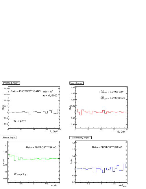
Figure 7: Ratios of results from PHOTOS with the excact correcting weight and SANC for the $W\to\mu\bar{\nu}(\gamma)$ decay distributions.

Now, let us consider the decay $W\to l\nu(\gamma)$. In [44] a simple correcting weight was introduced into PHOTOS for discrepancies with respect to exact predictions of SANC [53]. A weight based on the exact matrix element is presently available, see Appendix. One can check again how good approximation of ref. [44] is. As one can see from fig. 6 the correction weight reproduces the result of exact matrix element well. In fig. 7, we show that once the exact matrix element is implemented into PHOTOS the agreement with the benchmark calculation is better than the statistical error of $10^{8}$ events. In contrary to the previously studied $\gamma^{*}\to\pi^{+}\pi^{-}\gamma$ case, there were no problems of weight distribution tail.

Figure 1: Distributions of invariant masses normalized to center of mass energy and squared ($M^{\;2}/S$) for $e^{+}e^{-}\to\pi^{+}\pi^{-}(\gamma)$ at 2 GeV center of mass energy. Results from PHOTOS with matrix element taken from [38] are given in red (or darker grey) colour. If matrix element $\sum_{\lambda,\epsilon}|M_{I}^{\prime}|^{2}$ or $\sum_{\lambda,\epsilon}|M_{I^{\prime}}^{\prime}|^{2}$ is used (the two options are effectively identical) results are given in green colour. Logarithmic scale is used, but for the ratio (black line) linear scale is used instead. Fraction of events with photons above 50 MeV is respectively 4.2279 $\pm$ 0.0021 % and 4.2269 $\pm$ 0.0021% for the two programs.

\psfrag{M2pipi}{\scriptsize\bf$M_{\pi+\pi-}^{2}/S$}\psfrag{M2PiPlusGamma}{\scriptsize\bf$M_{\pi+\gamma}^{2}/S$}\includegraphics[width=208.13574pt]{one-a.eps}

(a) This distribution is identical to the distribution of photon energy in the reaction frame as well.

\psfrag{M2pipi}{\scriptsize\bf$M_{\pi+\pi-}^{2}/S$}\psfrag{M2PiPlusGamma}{\scriptsize\bf$M_{\pi+\gamma}^{2}/S$}\includegraphics[width=208.13574pt]{one-b.eps}

(b) This distribution coincides with distributions for squared invariant mass of $\pi^{-}\gamma$ pair.

Figure 2: Distributions of invariant masses normalized to center of mass energy and squared ($M^{\;2}/S$) for $e^{+}e^{-}\to\pi^{+}\pi^{-}(\gamma)$ at 2 GeV center of mass energy. Results from PHOTOS with matrix element taken from [38] are given in red colour. If matrix element $|M_{I}|^{2}$ is used results are given in green colour. Logarithmic scale is used, but for the ratio (black line) linear scale is used instead. Fraction of events with photons above 50 MeV is respectively 4.2279 $\pm$ 0.0021 % and 3.4435 $\pm$ 0.0019 % for the two programs.

\psfrag{M2pipi}{\scriptsize\bf$M_{\pi+\pi-}^{2}/S$}\psfrag{M2PiPlusGamma}{\scriptsize\bf$M_{\pi+\gamma}^{2}/S$}\includegraphics[width=208.13574pt,keepaspectratio]{two-a.eps}

(a) This distribution is identical to the distribution of photon energy in the reaction frame as well.

\psfrag{M2pipi}{\scriptsize\bf$M_{\pi+\pi-}^{2}/S$}\psfrag{M2PiPlusGamma}{\scriptsize\bf$M_{\pi+\gamma}^{2}/S$}\includegraphics[width=208.13574pt,keepaspectratio]{two-b.eps}

(b) It coincides with distributions for squared invariant mass of $\pi^{-}\gamma$ pair.

Figure 3: Distributions of invariant masses normalized to center of mass energy and squared ($M^{\;2}/S$) for $e^{+}e^{-}\to\pi^{+}\pi^{-}(\gamma)$ at 2 GeV center of mass energy. Results from PHOTOS with matrix element taken from [38] are given in red colour. If matrix element $\sum_{\lambda,\epsilon}|M_{I^{\prime}}|^{2}$ is used results are given in green colour. Logarithmic scale is used, but for the ratio (black line) linear scale is used instead. Fraction of events with photons above 50 MeV is respectively 4.2279 $\pm$ 0.0021 % and 3.8329 $\pm$ 0.0020 % for the two programs.

\psfrag{M2pipi}{\scriptsize\bf$M_{\pi+\pi-}^{2}/S$}\psfrag{M2PiPlusGamma}{\scriptsize\bf$M_{\pi+\gamma}^{2}/S$}\includegraphics[width=208.13574pt,keepaspectratio]{three-a.eps}

(a) This distribution is identical to the distribution of photon energy in the reaction frame as well.

\psfrag{M2pipi}{\scriptsize\bf$M_{\pi+\pi-}^{2}/S$}\psfrag{M2PiPlusGamma}{\scriptsize\bf$M_{\pi+\gamma}^{2}/S$}\includegraphics[width=208.13574pt,keepaspectratio]{three-b.eps}

(b) It coincides with distributions for squared invariant mass of $\pi^{-}\gamma$ pair.

Figure 4: Distributions of invariant masses normalized to center of mass energy and squared ($M^{\;2}/S$) for $e^{+}e^{-}\to\pi^{+}\pi^{-}(\gamma)$ at 2 GeV center of mass energy. Results from PHOTOS with matrix element taken from [38] are given in red colour. If complete matrix element is used results are given in green colour. Logarithmic scale is used, but for the ratio (black line) linear scale is used instead. Fraction of events with photons above 50 MeV is respectively 4.2279 $\pm$ 0.0021 % and 4.4320 $\pm$ 0.0021% for the two programs.

\psfrag{M2pipi}{\scriptsize\bf$M_{\pi+\pi-}^{2}/S$}\psfrag{M2PiPlusGamma}{\scriptsize\bf$M_{\pi+\gamma}^{2}/S$}\includegraphics[width=208.13574pt,keepaspectratio]{four-a.eps}

(a) This distribution is identical to the distribution of photon energy in the reaction frame as well.

\psfrag{M2pipi}{\scriptsize\bf$M_{\pi+\pi-}^{2}/S$}\psfrag{M2PiPlusGamma}{\scriptsize\bf$M_{\pi+\gamma}^{2}/S$}\includegraphics[width=208.13574pt,keepaspectratio]{four-b.eps}

(b) It coincides with distributions for squared invariant mass of $\pi^{-}\gamma$ pair.

Figure 5: Distributions of invariant masses normalized to center of mass energy and squared ($M^{\;2}/S$) for $e^{+}e^{-}\to\pi^{+}\pi^{-}(\gamma)$ at 2 GeV center of mass energy. Results from PHOTOS with matrix element taken from [38] are given in red colour. If exponentiation is activated as well results are given in green colour. Logarithmic scale is used, but for the ratio (black line) linear scale is used instead. Fraction of events with at least one photon above 50 MeV is respectively 4.2279 $\pm$ 0.0021 % and 4.1377 $\pm$ 0.0020% for the two cases.

\psfrag{M2pipi}{\scriptsize\bf$M_{\pi+\pi-}^{2}/S$}\psfrag{M2PiPlusGamma}{\scriptsize\bf$M_{\pi+\gamma}^{2}/S$}\includegraphics[width=208.13574pt,keepaspectratio]{exp-a.eps}

(a) This distribution is identical to the distribution of photon energy in the reaction frame as well.

\psfrag{M2pipi}{\scriptsize\bf$M_{\pi+\pi-}^{2}/S$}\psfrag{M2PiPlusGamma}{\scriptsize\bf$M_{\pi+\gamma}^{2}/S$}\includegraphics[width=208.13574pt,keepaspectratio]{exp-b.eps}

(b) It coincides with distributions for squared invariant mass of $\pi^{-}\gamma$ pair.

Figure 6: Ratios of results from PHOTOS with the old correcting weight and SANC for the $W\to\mu\bar{\nu}(\gamma)$ decay distributions.

5 Numerical results using beam direction

In the previous section we have discussed distributions regarding four-momenta of decay products only. Agreement between results of PHOTOS using universal kernel and simulations based on matrix element was excellent both in case of $W\to l\nu(\gamma)$ and $\gamma^{*}\to\pi^{+}\pi^{-}(\gamma)$ decays, even though the decaying particle spin effects were not taken into account in the PHOTOS kernel.

As can be seen from plots 8–11, distributions in variables sensitive to the orientation of the $W$ boson spin are affected. The plots 8 and 9 show distributions in the photon momentum angle with respect to a spin quantization axis as predicted by SANC and by PHOTOS with the standard kernel in transversally and longitudinally polarized W boson decays. The plots 10 and 11 correspond to the muon momentum orientation. The regions of phase space, where distributions are sparcely populated and where in fact at Born level probability density approach zero, are becoming moderately overpopulated by PHOTOS (increase of up to 14 % of density was found for transversely polarized $W$ boson decay). In most cases, this is probably of no practical consequences, nonetheless it requires quantification. Once the exact matrix element is implemented into PHOTOS, agreement with the SANC predictions is better than statistical error of $10^{8}$ events, see fig. 12.

Similar effects take place for $\gamma^{*}\to\pi^{+}\pi^{-}\gamma$. Even though from fig. 1 one could conclude that the universal kernel of [38], for arbitrary large samples, is equivalent to the matrix element as given by $\sum_{\lambda,\epsilon}|M_{I}^{\prime}|^{2}$ or $\sum_{\lambda,\epsilon}|M_{I^{\prime}}^{\prime}|^{2}$, differences appear in distributions sensitive to initial state spin orientation, see figs 13 and 14. On these plots angular distributions of the photon momentum with respect to the beam line are shown. Again, regions of phase space giving zero contribution at the Born level are becoming overpopulated if an approximation for the photon radiation matrix element is used. From that perspective and for practical reasons one can conclude that the $\sum_{\lambda,\epsilon}|M_{I^{\prime}}^{\prime}|^{2}$ choice is better than $\sum_{\lambda,\epsilon}|M_{I}^{\prime}|^{2}$. It yelds distributions closer to the ones obtained from universal kernel. Then, the remaining part of (19) represents better correction to implement bulk of effects from complete matrix element to events generated with default PHOTOS. We can see also that distributions obtained from kernel of ref. [38] and $\sum_{\lambda,\epsilon}|M_{I}^{\prime}|^{2}$ are close to each other but nonetheless distinct. Complete implementation requires control of the $\gamma^{*}$ spin. The Born level distribution for $\gamma^{*}$ decay has zero at $\cos\theta_{\pi^{\pm}}=\pm 1$. Close to these directions internal weight of PHOTOS necessary for exact matrix element becomes large, see figs. 13,14. Zero which is also present in distribution of Born level $W$ decay is of no such consequences for the weight distribution.

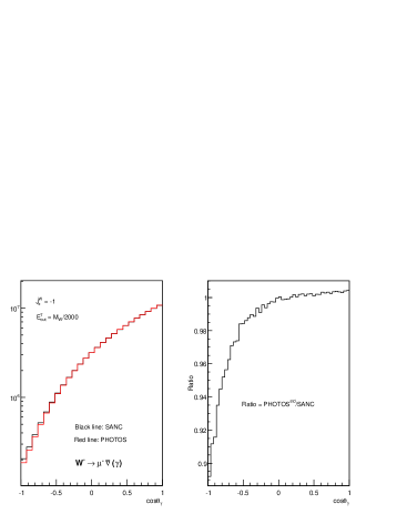
Figure 8: Cosine of the angle of photon momentum with respect to spin axis in the decay $W\to\mu\bar{\nu}(\gamma)$. W boson is transversely polarized, $J^{W}_{z}=-1$. The black line corresponds to SANC results, while the red line corresponds to predictions of PHOTOS with standard kernel.

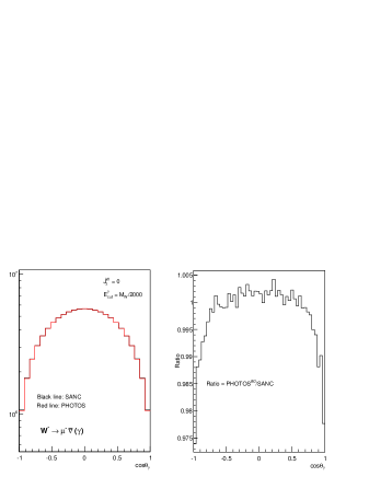
Figure 9: Cosine of the angle of photon momentum with respect to spin axis in the decay $W\to\mu\bar{\nu}(\gamma)$. W boson is longitudinally polarized, $J^{W}_{z}=0$. The black line corresponds to SANC results, while the red line corresponds to predictions of PHOTOS with standard kernel.

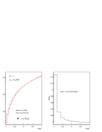
Figure 10: Cosine of the angle of muon momentum with respect to spin axis in the decay $W\to\mu\bar{\nu}(\gamma)$ is shown. W boson is transversally polarized, $J^{W}_{z}=-1$. The black line corresponds to SANC results, while the red line corresponds to predictions of PHOTOS with standard kernel. Comparison of the distributions show that lack of spin effects in PHOTOS standard kernel results in up to 14% surplus of events for phase-space region close to $\cos\theta_{\mu}=-1$.

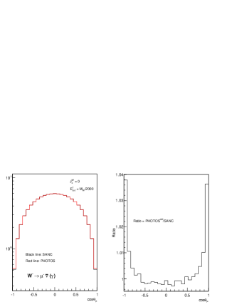
Figure 11: Cosine of the angle of the muon momentum with respect to spin axis in the decay $W\to\mu\bar{\nu}(\gamma)$ is shown. W boson is longitudinally polarized, $J^{W}_{z}=0$. The black line corresponds to SANC results, while the red line corresponds to predictions of PHOTOS with standard kernel. Comparison of the distributions show that lack of spin effects in PHOTOS standard kernel results in up to 4% surplus of events for phase-space region close to $\cos\theta_{\mu}=\pm 1$.

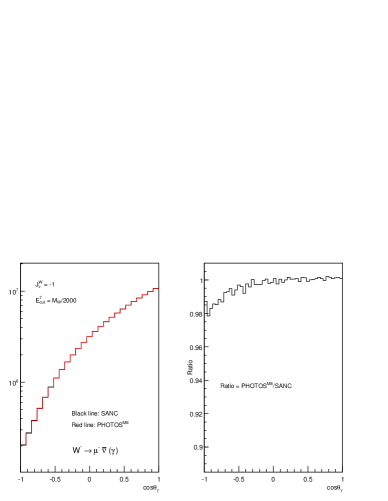
Figure 12: Cosine of the angle of photon momentum with respect to spin axis in the decay $W\to\mu\bar{\nu}(\gamma)$ is shown. W boson is transversely polarized, $J^{W}_{z}=-1$, along this axis. The black line corresponds to SANC results, while the red line corresponds to predictions of PHOTOS with exact matrix element.

Figure 13: Angular distributions for $e^{+}e^{-}\to\pi^{+}\pi^{-}(\gamma)$ at 2 GeV center of mass energy. Results from PHOTOS with matrix element taken from [38] are given in red colour. Matrix element $\sum_{\lambda,\epsilon}|M_{I}^{\prime}|^{2}$ is used for results with green line. Logarithmic scale is used, but for the ratio (black line) linear scale is used instead. Fraction of presented events (i.e. with photons above 50 MeV) is respectively 4.2279 $\pm$ 0.0021 % and 4.2269 $\pm$ 0.0021% of the total samples for the two programs.

\psfrag{cosThetaGamma}{\scriptsize$\cos\theta_{\gamma}$}\psfrag{cosThetaPiPlus}{\scriptsize$\cos\theta_{\pi+}$}\includegraphics[width=212.47617pt,keepaspectratio]{one-c.eps}

(a) cosine of the photon angle with respect to beam.

\psfrag{cosThetaGamma}{\scriptsize$\cos\theta_{\gamma}$}\psfrag{cosThetaPiPlus}{\scriptsize$\cos\theta_{\pi+}$}\includegraphics[width=212.47617pt,keepaspectratio]{one-d.eps}

(b) cosine of the $\pi^{+}$ angle with respect to the same charge beam.

Figure 14: Angular distributions for $e^{+}e^{-}\to\pi^{+}\pi^{-}(\gamma)$ at 2 GeV center of mass energy. Results from PHOTOS with matrix element taken from [38] are given in red colour. $\sum_{\lambda,\epsilon}|M_{I^{\prime}}^{\prime}|^{2}$ is used for results with green line. Logarithmic scale is used, but for the ratio (black line) linear scale is used instead. Fraction of presented events (i.e. with photons above 50 MeV) is respectively 4.2279 $\pm$ 0.0021 % and 4.2271 $\pm$ 0.0021% of the total samples for the two programs.

\psfrag{cosThetaGamma}{\scriptsize$\cos\theta_{\gamma}$}\psfrag{cosThetaPiPlus}{\scriptsize$\cos\theta_{\pi+}$}\includegraphics[width=212.47617pt,keepaspectratio]{one-cc.eps}

(a) cosine of the photon angle with respect to beam is shown.

\psfrag{cosThetaGamma}{\scriptsize$\cos\theta_{\gamma}$}\psfrag{cosThetaPiPlus}{\scriptsize$\cos\theta_{\pi+}$}\includegraphics[width=212.47617pt,keepaspectratio]{one-dd.eps}

(b) cosine of the $\pi^{+}$ angle with respect to the same charge beam is shown.

6 Summary

In this paper we have studied matrix elements for the $\gamma^{*}\to\pi^{+}\pi^{-}\gamma$ and $W\to l\nu\gamma$ processes. We have observed that the expressions can be separated into gauge invariant parts. In both cases, the part consisting of eikonal factor multiplying the Born level spin amplitude separates. This part contributes to the infrared singularity. In the case of $\gamma^{*}\to\pi^{+}\pi^{-}\gamma$ the remaining part does not contribute to collinear singularity but for $W\to l\nu$ it can be separated further: into the part proportional to the $W$ charge which does not lead to any logarithmic contribution after integration, and the part proportional to the lepton charge, which do contribute to collinear singularity and is identical to an analogous part for the $Z\to l^{+}l^{-}$ process (see eg. second or third part of formula 5 in [27]). This is exactly the factorization property needed for the iterative solution used in PHOTOS to be valid for multiphoton emissions and processes discussed in present paper.

For $\gamma^{*}\to\pi^{+}\pi^{-}\gamma$, the factor, identified as Born level amplitude is not unique. As expected, ambiguity is proportional to photon momentum, and disappears in the soft limit. As a consequence of the ambiguity options were discussed. Their difference is of no practical consequences for the present work, but should be kept in mind if the obtained spin amplitude parts would be used as building bricks for amplitudes of more elaborated processes.

We have identified dominant parts of spin amplitudes and used them for tests and for kernels of PHOTOS Monte Carlo. Exact matrix element was used for that purpose. We have found, that the whole matrix element for the process $W\to l\nu\gamma$ can be incorporated into the photon emission kernel. However for $\gamma^{*}\to\pi^{+}\pi^{-}\gamma$ it is not technically straightforward, because of large weight events. The responsible term was identified and it may be interesting to point out that it is similar to the one obtained in a different calculation (Ref. [27] equation (68)). There, such terms were interpreted as contributing to running of QCD coupling constant. In present calculation the term involves complete kinematics of $\gamma^{*}\to\pi^{+}\pi^{-}\gamma$ process.

Any further investigation of the analogy, would require amplitudes of higher orders. Such effort can not be justified for scalar QED. From low energy point of view, terms like (12) or (14) should be understood as genuine scalar QED process, and not part of real photon bremsstrahlung. Scalar QED is not supposed to be valid in the regions of phase space where these terms contribute significantly. It is of phenomenological interest to check this limit of scalar QED predictions by direct comparisons with data. Thanks to present work, higher order genuine bremsstrahlung effects for $\gamma^{*}\to\pi^{+}\pi^{-}\gamma$ can be simulated with the help of PHOTOS and one can concentrate on confronting the data with these non-bremsstrahlung parts (12) or (14).

We have neither discussed here the interference with the photons originating from incoming beams, nor the interference between two consecutive emissions from the same charged line. The first effect, requires simultaneous treatment of initial-state and final-state bremsstrahlung. This is out of scope of work on PHOTOS alone, but spin amplitudes are already prepared. For discussion of interference of two emissions from the same charged line (and resulting uncertainties) second order matrix element is needed. Fortunately the structure of spin amplitudes for $\gamma^{*}\to\pi^{+}\pi^{-}\gamma$ and $W\to l\nu$ matches that of $Z\to l^{+}l^{-}\gamma$ [33]. At present, we can only expect that these results on $Z\to l^{+}l^{-}\gamma$ in combination with our algorithm for matching consecutive emissions, hold for our $\gamma^{*}\to\pi^{+}\pi^{-}$ processes. Results of Ref. [54] point that this expectation is well founded.

We have not discussed virtual corrections. We assume, following Kinoshita-Lee-Nauenberg theorem [48, 49], that the dominant part can be included in a factor multiplying Born amplitude and the correction to the total rate is free of any large logarithm. We leave this point for future work.

Finally, this paper provides numerical tests of PHOTOS Monte Carlo, in particular construction for decays where Born level cross section has a zero. This is of practical interest for users of the program and also a necessary step before any attempt of an extension to QCD.

Appendix A Matrix element for W decay

The matrix element of the process $W^{-}(Q,\lambda)\rightarrow l(p_{l},\lambda_{l})\,\bar{\nu}(p_{\nu},\lambda_{\nu})\,\gamma(k,\sigma)$ has the form

$$\textit{M}^{\,\sigma}_{\lambda,\lambda_{\nu},\lambda_{l}}(k,Q,p_{\nu},p_{l}) = \left[\frac{Q_{l}}{2\,k\cdot p_{l}}b_{\sigma}(k,p_{l})-\frac{Q_{W}}{2\,k\cdot Q}\left(b_{\sigma}(k,p_{l})+b_{\sigma}(k,p_{\nu})\right)\right]{\textit{\large B}^{\lambda}_{\lambda_{l},\lambda_{\nu}}(p_{l},Q,p_{\nu})}$$

$$+\frac{Q_{l}}{2\,k\cdot p_{l}}\sum_{\rho=\pm}U^{\sigma}_{\lambda_{l},\rho}(p_{l},m_{l},k,0,k,0){\textit{\large B}^{\lambda}_{\rho,-\lambda_{\nu}}(k,Q,p_{\nu})}$$

$$-\frac{Q_{W}}{2\,k\cdot Q}\sum_{\rho=\pm}\left({\textit{\large B}^{\lambda}_{\lambda_{l},-\rho}(p_{l},Q,k)}{U^{\sigma}_{-\rho,-\lambda_{\nu}}(k,0,k,0,p_{\nu},0)}\right.$$

$$\left.\phantom{xxxxxxxxxx}+U^{\sigma}_{\lambda_{l},\rho}(p_{l},m_{l},k,0,k,0){\textit{\large B}^{\lambda}_{\rho,-\lambda_{\nu}}(k,Q,p_{\nu})}\right),$$

where we use the following notation :

$$\textit{\large B}^{\lambda}_{\lambda_{1},\lambda_{2}}(p_{1},Q,p_{2}) \equiv \frac{g}{2\sqrt{2}}\bar{u}(p_{1},\lambda_{1})\,\widehat{\epsilon}^{\lambda}_{W}(Q)(1+\gamma_{5})\,v(p_{2},\lambda_{2})\,,$$

$$U^{\sigma}_{\lambda_{1},\lambda_{2}}(p_{1},m_{1},k,0,p_{2},m_{2}) \equiv \bar{u}(p_{1},\lambda_{1})\,\widehat{\epsilon}^{\sigma}_{\gamma}(k)\,u(p_{2},\lambda_{2})\,,$$ (33)

$$\delta_{\lambda_{1}\lambda_{2}}b_{\sigma}(k,p) \equiv U^{\sigma}_{\lambda_{1},\lambda_{2}}(p,m,k,0,p,m)\,,$$

$Q_{l}$ and $Q_{W}$ are respectively the electric charges of the fermion $l$ and the $W$ boson, in units of the positron charge, ${\epsilon}^{\sigma}_{\gamma}(k)$ and ${\epsilon}^{\lambda}_{W}(Q)$ denote respectively the polarization vectors of the photon and the $W$ boson. An expression of the function $U^{\sigma}_{\lambda_{1},\lambda_{2}}$ in terms of the massless spinors and other notations can be found in [52]. It is easy to check that the three components of the sum contributing to (A) are individually gauge invariant. Note, that the first component coincides with the amplitude in the eikonal approximation.

References

• [1] R. Kleiss, ed., oai:cds.cern.ch:367653. Workshop on Z Physics at LEP1 : General Meetings, v.3 : Z physics at LEP 1 - Event generators and software. Coordinated and supervised by R. Kleiss.
• [2] S. Jadach, G. Passarino, and R. Pittau, eds., Reports of the working groups on precision calculation for LEP-2 physics. Proceedings, Monte Carlo Workshop, Geneva, Switzerland, 1999-2000.
• [3] M. Kobayashi, Nobel Prize Lecture: CP Violation and Flavor Mixing.
• [4] Belle Collaboration, K. Abe et al., Phys. Rev. Lett. 98 (2007) 181804, hep-ex/0608049.
• [5] BABAR Collaboration, B. Aubert et al., Phys. Rev. D67 (2003) 032002, hep-ex/0207097.
• [6] F. A. Berends, R. Kleiss, and S. Jadach, Comput. Phys. Commun. 29 (1983) 185–200.
• [7] S. Jadach, B. F. L. Ward, and Z. Was, Comput. Phys. Commun. 66 (1991) 276–292.
• [8] T. Sjostrand, Comput. Phys. Commun. 82 (1994) 74–90.
• [9] G. Corcella et al., JHEP 01 (2001) 010, hep-ph/0011363.
• [10] D. R. Yennie, S. C. Frautschi, and H. Suura, Ann. Phys. 13 (1961) 379–452.
• [11] S. Jadach, MPI-PAE/PTh 6/87.
• [12] S. Jadach, B. F. L. Ward, and Z. Was, Phys. Rev. D63 (2001) 113009, hep-ph/0006359.
• [13] E. A. Kuraev, L. N. Lipatov, and V. S. Fadin, Sov. Phys. JETP 44 (1976) 443–450.
• [14] E. A. Kuraev, L. N. Lipatov, and V. S. Fadin, Sov. Phys. JETP 45 (1977) 199–204.
• [15] I. I. Balitsky and L. N. Lipatov, Sov. J. Nucl. Phys. 28 (1978) 822–829.
• [16] V. S. Fadin and L. N. Lipatov, Phys. Lett. B429 (1998) 127–134, hep-ph/9802290.
• [17] B. I. Ermolaev, M. Greco, and S. I. Troyan, Acta Phys. Polon. B38 (2007) 2243–2260, 0704.0341.
• [18] V. G. Gorshkov, V. N. Gribov, L. N. Lipatov, and G. V. Frolov, Sov. J. Nucl. Phys. 6 (1968) 262.
• [19] V. G. Gorshkov, V. N. Gribov, L. N. Lipatov, and G. V. Frolov, Sov. J. Nucl. Phys. 6 (1968) 95.
• [20] L. V. Gribov, E. M. Levin, and M. G. Ryskin, Phys. Rept. 100 (1983) 1–150.
• [21] B. R. Webber, Ann. Rev. Nucl. Part. Sci. 36 (1986) 253–286.
• [22] B. I. Ermolaev, M. Greco, and S. I. Troyan, Phys. Lett. B522 (2001) 57–66, hep-ph/0104082.
• [23] B. I. Ermolaev and S. I. Troyan, Phys. Lett. B666 (2008) 256–261, 0805.2278.
• [24] CDF Collaboration, A. A. Affolder et al., Phys. Rev. D65 (2002) 092002.
• [25] M. Derrick and T. Gottschalk, Contributed to Summer Study on the Design and Utilization of the Superconducting Super Collider, Snowmass, Colo., Jun 23-Jul 13, 1984.
• [26] L. Berny, Z. Phys. C48 (1990) 227–229.
• [27] A. van Hameren and Z. Was, Eur. Phys. J. C61 (2009) 33–49, 0802.2182.
• [28] E. Barberio, B. van Eijk, and Z. Was, Comput. Phys. Commun. 66 (1991) 115–128.
• [29] E. Barberio and Z. Was, Comput. Phys. Commun. 79 (1994) 291–308.
• [30] F. A. Berends, R. Kleiss, and S. Jadach, Nucl. Phys. B202 (1982) 63.
• [31] E. Richter-Was and Z. Was, CPT-87/P-2080.
• [32] S. Jadach, B. F. L. Ward, and Z. Was, Comput. Phys. Commun. 130 (2000) 260–325, hep-ph/9912214.
• [33] Z. Was, Eur. Phys. J. C44 (2005) 489–503, hep-ph/0406045.
• [34] E. Richter-Was, Z. Phys. C64 (1994) 227–240.
• [35] E. Richter-Was, Z. Phys. C61 (1994) 323–340.
• [36] P. Golonka and Z. Was, Eur. Phys. J. C45 (2006) 97–107, hep-ph/0506026.
• [37] P. Golonka and Z. Was, Eur. Phys. J. C50 (2007) 53–62, hep-ph/0604232.
• [38] G. Nanava and Z. Was, Eur. Phys. J. C51 (2007) 569–583, hep-ph/0607019.
• [39] P. Golonka, T. Pierzchala, and Z. Was, Comput. Phys. Commun. 157 (2004) 39–62, hep-ph/0210252.
• [40] N. Davidson, P. Golonka, T. Przedzinski, and Z. Was, 0812.3215.
• [41] V. N. Gribov and L. N. Lipatov, Sov. J. Nucl. Phys. 15 (1972) 438–450.
• [42] J. C. Collins, D. E. Soper, and G. Sterman, Nucl. Phys. B261 (1985) 104.
• [43] A. Andonov, S. Jadach, G. Nanava, and Z. Was, Acta Phys. Polon. B34 (2003) 2665–2672, hep-ph/0212209.
• [44] G. Nanava and Z. Was, Acta Phys. Polon. B34 (2003) 4561–4570, hep-ph/0303260.
• [45] G. Rodrigo, H. Czyz, J. H. Kuhn, and M. Szopa, Eur. Phys. J. C24 (2002) 71–82, hep-ph/0112184.
• [46] D. Bardin, S. Jadach, T. Riemann, and Z. Was, Eur. Phys. J. C24 (2002) 373–383, hep-ph/0110371.
• [47] F. A. Berends, R. Kleiss, J. P. Revol, and J. P. Vialle, Z. Phys. C27 (1985) 155.
• [48] T. Kinoshita, J. Math. Phys. 3 (1962) 650.
• [49] T. D. Lee and M. Nauenberg, Phys. Rev. B133 (1964) 1549.
• [50] H. Czyz, A. Grzelinska, J. H. Kuhn, and G. Rodrigo, Eur. Phys. J. C27 (2003) 563–575, hep-ph/0212225.
• [51] S. Jadach, E. Richter-Was, B. F. L. Ward, and Z. Was, Phys. Lett. B253 (1991) 469–477.
• [52] S. Jadach, B. F. L. Ward, and Z. Was, Phys. Lett. B449 (1999) 97–108, hep-ph/9905453.
• [53] A. Andonov et al., Comput. Phys. Commun. 174 (2006) 481–517, hep-ph/0411186.
• [54] G. Isidori, Eur. Phys. J. C53 (2008) 567–571, 0709.2439.