Universality and the zero-bias conductance of the single-electron transistor

Abstract

The thermal dependence of the electrical conductance of the single-electron transistor (SET) in the zero-bias Kondo regime is discussed. An exact mapping to the universal curve for the symmetric Anderson model is established. Linear, the mapping is parametrized by the Kondo temperature and the charge in the Kondo cloud. Illustrative numerical renormalization-group results, in excellent agreement with the mapping, are presented.

Nearly five decades ago, Anderson conceived a Hamiltonian to describe the interaction between a magnetic impurity and otherwise free conduction electrons.Anderson (1961) Once a daunting theoretical challenge, the Anderson Hamiltonian yielded to an essentially exact numerical diagonalization,Krishna-murthy et al. (1980a) followed by an exact analytical diagonalization.Andrei et al. (1983); Tsvelick and Wiegmann (1983) From these and alternative approaches, physical properties were extracted, which eased the interpretation of experimental data;Goldhaber-Gordon et al. (1998a) theoretical results provided unifying views of apparently unrelated phenomena;Wilkins (1982) and quantitative comparisons brought forth novel perceptions.Lin et al. (1987)

The last ten years were especially fruitful. Parallel advances in scanning tunneling spectroscopy and in the fabrication of nanostructured semiconductor devices enhanced the interest in transport properties.Madhavan et al. (1998); van der Wiel et al. (2000); Hofstetter et al. (2001); van der Wiel et al. (2003); Agrait et al. (2003); Kirchner et al. (2005); Crommie (2005); Franco et al. (2003); Romeike et al. (2006); Dias da Silva et al. (2006); Zitko and Bonca (2006); Dias da Silva et al. (2008) In both areas, numerous experimental breakthroughs and theoretical analyses were reported, and the Anderson Hamiltonian proved spectacularly successful in more than one occasion.Oreg and Goldhaber-Gordon (2003); Fu et al. (2007)

Notwithstanding the substantial volume of exact results, certain aspects of the model remain obscure. Consider universality, a concept important in its own right and by virtue of its diverse applications. Universal relations serve as benchmarks checking the accuracy of numerical data; as resources promoting the convergence of theoretical findings; and as instruments bridging the gap between the theorist’s tablet and the laboratory logbook. The conditions under which the Anderson model exhibits universal thermodynamical properties were identified.Krishna-murthy et al. (1980a); Andrei et al. (1983); Tsvelick and Wiegmann (1983) Although one expects all properties of the model to be universal in the same domain, few firm results for the dynamical and transport properties can be found in libraries.Bulla et al. (2008) Costi’s et al’s early effort showed that the transport coefficients for the symmetric Anderson model are universal.Costi et al. (1994) For asymmetric models—even ones that display universal thermodynamical properties—, nonetheless, the universal curves fail to fit the numerical data, the disagreement growing with the (particle-hole) asymmetry.

Puzzled by such contrasts, we have conducted a systematic study of the transport properties for the Anderson Hamiltonian. We combined analytical and numerical-renormalization group (NRG) tools and paid special attention to universality. In a preliminary report,Seridonio et al. (2007) we have discussed an Anderson model for a quantum dot side-coupled to a quantum wire, a device comprising two conduction paths whose transport properties are marked by interference.Kobayashi et al. (2004); Sato et al. (2005); Katsumoto et al. (2006); Otsuka et al. (2007); Katsumoto (2007) Notwithstanding the constructive or destructive effects, we have been able to identify universal behavior throughout the Kondo regime, the parametrical domain favoring the formation of a magnetic moment at the quantum dot and its progressive screening by the conduction electrons as the temperature is lowered past the scale set by the Kondo temperature $T_{K}$. Specifically, we found the thermal dependence of the conductance to map linearly onto a universal function of the temperature $T$ scaled by the Kondo temperature $T_{K}$. The mapping is itself universal, i. e., it depends on a single physical property, the ground-state phase shift $\delta$, into which the contributions from all model parameters are lumped.

This report examines the alternative experimental set-up in which a quantum dot or molecule, instead of side-coupled to, is embedded in the conduction path.Goldhaber-Gordon et al. (1998b, c); Göres et al. (2000); Liang et al. (2002); Oreg and Goldhaber-Gordon (2003); Yu et al. (2004, 2005); Kirchner et al. (2005) We show that the thermal dependence of the conductance maps onto the same universal function. Although linear, the mapping now depends explicitly on a model parameter—an external potential applied to the conduction electrons—and hence contrasts with the conclusion in our previous report. This dependence accounts for distinctions between the transport properties in the embedded and side-coupled arrangements. At high temperatures, for instance, potentials appropriately applied to the conduction electrons in the side-coupled geometry drive the conductance from low values up to the ballistic limit ${\mathcal{G}}_{2}=2e^{2}/h$. If the quantum dot is embedded in the conduction path, by contrast, the high-temperature conductance is pinned at low values and virtually insensitive to potentials applied to the conduction electrons. Our analysis shows that, in the embedded configuration, the screening charge in the Kondo cloud parametrizes the mapping to the universal conductance curve. Since that charge is always close to unity, the mapping is never far from the identity, with maximum relative deviations around 20%.

Our presentation focuses the mapping between the SET and the universal conductances. As illustrations we will present the results of a few Numerical Renormalization Group (NRG) runs. A discussion of the numerics, a comprehensive survey of the Kondo regime, and the comparison with the side-coupled geometry will be deferred to another report.

The text is divided in five Sections, more technical aspects of the analysis having been confined to the three Appendices. Section I defines the model. Section II derives an expression relating the conductance to the spectral density of the quantum dot level. Section III is dedicated to universality, and Section IV, to the fixed points of the model Hamiltonian and to an extension of Langreth’s exact expression for the ground-state spectral density. Section V then shows that, in the Kondo regime, the thermal dependence of the conduction can be mapped onto the symmetric-SET universal conductance. Finally, Section VI collects our conclusions.

I Single-electron transistor

Figure 1 depicts a single-electron transistor (SET), the prototypical example of embedding. The subject of numerous experimental studies, the SET comprises two independent conduction bands coupled by a localized level.

Figure 1: Single-electron transistor. A quantum dot (circle) bridges two quantum wires (rectangles). A gate potential $V_{d}$ controls the dot energy, while the symmetric potentials $V_{w}$ shift the the energy of the wire orbitals close to the dot.

Qualitatively, the physics of Fig. 1 was understood long before the first device was developed. Figure 2 displays the spectrum of the SET Hamiltonian $H$ for zero coupling. The dot levels being then decoupled from the conduction bands, the eigenstates and eigenvalues of $H$ can be labeled by the dot quantum numbers. For simplicity, we will only refer to the dot occupation $n_{d}$. For fixed $n_{d}$, the product of the lowest dot state by the conduction-band ground state is shown as a bold dash. The gray levels above it represent the excited states consistent with the same $n_{d}$ label.

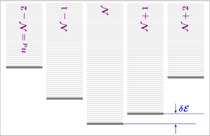
Figure 2: SET energies in the weak-coupling limit. The dot-level occupation $n_{d}$ labels the energies. For each $n_{d}$, the bold dash represents the conduction-band ground state, while the thinner lines represent excitations. The coupling between the dot and the two quantum wires mixes each level to the neighboring columns.

A small transition amplitude $V$ between the quantum dot and the wires is sufficient to modify this picture. The amplitude $V$ couples strongly each gray level to the degenerate or nearly degenerate states in the neighboring columns. Exceptions are the lowest levels in the column labeled $n_{d}=\mathcal{N}$ in Fig. 2, which are energetically distant from their neighbors and thus remain unperturbed to first order in the coupling. At low temperatures, with $k_{B}T$ small in comparison with the energy $\delta\mathcal{E}$ separating the ground state from the closest level in the neighboring columns, the dot occupation is frozen at $n_{d}=\mathcal{N}$, a constraint that raises the Coulomb blockade against conduction through the dot.

Adjustment of the gate potential $V_{d}$ in Fig. 1 brings down the blockade. The potential shifts the energies of the dot levels and can be tuned to the condition $\delta\mathcal{E}\approx 0$, to impose degeneracy between the bold dashes in the $n_{d}=\mathcal{N}$ and $n_{d}=\mathcal{N}+1$ columns. An infinitesimal bias is then sufficient to induce electronic flow between the wires throught the dot. The conductance peak, we see, at gate potentials $V_{d}$ such that the ground-state expectation value of $n_{d}$ is half-integer, e. g., $\langle\Omega|\,n_{d}\,|\Omega\rangle=\mathcal{N}+1/2$ as $\delta\mathcal{E}\to 0$ in Fig. 2.

Each peak identifies a resonance at the Fermi level. As the gate voltage is swept past $\delta\mathcal{E}=0$, the ground-state occupation changes rapidly from $n_{d}=\mathcal{N}$ to $n_{d}=\mathcal{N}+1$, and as required by the Friedel sum rule, so does the ground-state phase shift. At moderately low temperatures, for thermal energies smaller than the average spacing between the bold dashes in the figure, the plot of the conductance as a function of the gate voltage is a succession of peaks. Data collected in the laboratory at moderately low temperatures do display a sequence of resonances. At very low temperatures, however, the pattern changes to a sequence of intervals alternating between insulation and conduction.

The conducting plateaus are due to the Kondo effect. For gate voltages corresponding to odd ground-state dot occupations, the magnetic moment of the resulting dot spin interacts antiferromagnetically with the conduction electrons. As the device is cooled past the Kondo temperature, the screening of the moment creates the Kondo resonance, a spiked enhancement of the density of states pinned at the Fermi level. Notwithstanding the Coulomb blockade, the pinned resonance allows conduction.

II Anderson model

A variant of the Anderson Hamiltonian encapsulates the physics of the device in Fig. 1. A spin degenerate level $c_{d}$ represents the dot level, and two structureless half-filled conduction bands, labeled $L$ (left) and $R$ (right), represent the two quantum wires. The $L$ ($R$) wire comprises $N$ state $c_{kL}$ ($c_{kR}$) with energies defined by the linear dispersion relation $\epsilon_{k}=(k-k_{F})v_{F}$ ($0\leq k\leq 2k_{F}$), so that the bandwidth is $2D=2v_{F}k_{F}$. The per-particle, per-spin density of conduction states is $\rho=1/2D$, and we will let $\Delta\equiv D/N$ denote the energy splittings in the conduction bands. The model Hamiltonian is then the sum of three terms, $H=H_{w}+H_{d}+H_{wd}$, where the first term describes the wires:

$$H_{w}=\sum_{k\alpha}\epsilon_{k}c_{k\alpha}^{\dagger}c_{k\alpha}+\frac{W}{N}\sum_{kq\alpha}c_{k\alpha}^{\dagger}c_{q\alpha},$$ (1)

with an intra-wire scattering potential $W$, fixed by the potential $V_{w}$ in Fig. 1, and $\alpha=L,R$. The Hamiltonian $H_{d}$ describes the dot:

$$H_{d}=\varepsilon_{d}n_{d}+Un_{d\uparrow}n_{d\downarrow},$$ (2)

with a dot energy $\varepsilon_{d}$ controlled by the gate potential $V_{d}$ in Fig. 1; and the Hamiltonian $H_{wd}$ couples the wires to the dot:

$$H_{wd}=\frac{V}{\sqrt{2N}}\sum_{k\alpha}(c_{k\alpha}^{\dagger}c_{d}+{\text{H.\ c.}}).$$ (3)

II.1 Parity

To exploit the inversion symmetry of Fig. 1, we define the normalized even ($a_{k}$) and odd ($b_{k}$) operators

$$a_{k}=\frac{1}{\sqrt{2}}(c_{kL}+c_{kR});$$ (4a)

$$b_{k}=\frac{1}{\sqrt{2}}(c_{kL}-c_{kR}).$$ (4b)

The projection of the model Hamiltonian on the basis of the $a_{k}$’s and $b_{k}$’s splits it in two decoupled pieces, $H=H_{A}+H_{B}$, where

$$H_{A}=\sum_{k}\epsilon_{k}a_{k}^{\dagger}a_{k}+Wf_{0}^{\dagger}f_{0}+V(f_{0}^{\dagger}c_{d}+{\text{H.\ c.}})+H_{d},$$ (5)

where we have introduced the traditional NRG shorthand

$$f_{0}\equiv\sum_{k}a_{k}/{\sqrt{N}},$$ (6)

and

$$H_{B}=\sum_{k}\epsilon_{k}b_{k}^{\dagger}b_{k}+\frac{W}{N}\sum_{kq}b_{k}^{\dagger}b_{q}.$$ (7)

II.2 Conductance

The odd Hamiltonian $H_{B}$ is decoupled from the quantum dot. It is, moreover, quadratic, and hence easily diagonalizable. Appendix C determines its spectrum, analyzes the response of the conduction and dot electrons to the application of an infinitesimal bias and turns the result into the following Linear Response expression for the conductance:

$$G(T)={\mathcal{G}}_{2}\,\pi\Gamma_{W}\,\int_{-D}^{D}\rho_{d}(\epsilon,T)\left[-\frac{\partial f(\epsilon)}{\partial\epsilon}\right]\,d\epsilon,$$ (8)

where $f(\epsilon)$ is the Fermi function;

$$\Gamma_{W}=\frac{\Gamma}{1+\pi^{2}\rho^{2}W^{2}}$$ (9)

is the width $\Gamma=\pi\rho V^{2}$ of the $c_{d}$ level, here renormalized by the scattering potential $W$; and

$$\rho_{d}(\epsilon,T)=\frac{1}{f(\epsilon)}\sum_{mn}\frac{e^{-\beta E_{m}}}{\mathcal{Z}}|\langle n|\,c_{d}^{\dagger}\,|m\rangle|^{2}\delta(\epsilon_{mn}-\epsilon)$$ (10)

is the spectral density for the dot level. Here $|m\rangle$ and $|n\rangle$ are eigenstates of $H_{A}$ with eigenvalues $E_{m}$ and $E_{n}$, respectively, $\epsilon_{mn}\equiv E_{m}-E_{n}$, and $\mathcal{Z}$ is the partition function for the Hamiltonian $H_{A}$.

As one would expect, given that the odd Hamiltonian $H_{B}$ commutes with $c_{d}$, only the eigenvalues and eigenvectors of $H_{A}$ are needed to compute the right-hand side of Eqs. (8) and (10). The following discussion will hence focus the even Hamiltonian, Eq. (5), which is equivalent to the conventional spin-degenerate Anderson Hamiltonian.Anderson (1961)

II.3 Characteristic energies

Four characteristic energies govern the physical properties of the Anderson Hamiltonian. Two of them are displayed in Fig. 3: the energy $-\epsilon_{d}$ needed to remove an electron from the dot level; and the energy $\epsilon_{d}+U$ needed to add an electron to the level. The particle-hole transformation $c_{k}\to c_{k}^{\dagger}$; $c_{d}\to-c_{d}^{\dagger}$ swaps the two energies, so that, the transformed dot Hamiltonian is given by the right-hand side of Eq. (2) with $\epsilon_{d}\to-(\epsilon_{d}+U)$.

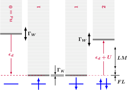
Figure 3: Spectrum of the spin-degenerate Anderson model, displayed as in Fig. 2. In the weak-coupling limit, the eigenstates are labeled by the occupation $n_{d}$ and spin component of the dot configuration displayed at the bottom. For $V\neq 0$, each level in the left and right columns hybridizes with nearly degenerate levels in the central columns and acquires the width $\Gamma_{W}$ in Eq. (9). At low energies, the levels in the two central columns combine into a singlet and acquire a width $\Gamma_{K}\sim k_{B}T_{K}$.The vertical arrows near the right border mark the domains of the LM and FL fixed points.

If $2\epsilon_{d}+U=0$, the dot Hamiltonian remains invariant under the particle-hole transformation. If, in addition, $W=0$, Eq. (5) reduces to the symmetric Hamiltonian

$$H_{A}^{S}=\sum_{k}\epsilon_{k}a_{k}^{\dagger}a_{k}+V(f_{0}^{\dagger}c_{d}+{\text{H.\ c.}})-\frac{U}{2}(n_{d\uparrow}-n_{d\downarrow})^{2}.$$ (11)

With $V\neq 0$, two other energies arise: the level width $\Gamma_{W}$ [Eq. (9)] and the Kondo energy $k_{B}T_{K}$, given by

$$T_{K}\sim\sqrt{\rho J}\exp(-1/\rho J),$$ (12)

where $J$ is the antiferromagnetic interaction between the conduction electrons and the dot magnetic moment,Schrieffer and Wolff (1966)

$$\rho J=2\frac{\Gamma_{W}}{\pi|\varepsilon_{d}|}\frac{U}{\varepsilon_{d}+U}.$$ (13)

In the Kondo regime, thermal and excitation energies are much smaller than $\min(|\varepsilon_{d}|,\varepsilon_{d}+U)$. In Fig. 3, only the lowest levels in the central columns are energetically accessible. The energy $\Gamma_{W}$, associated with transitions from the central to the external columns in the figure (i. e., with $c_{d}^{1}\to c_{d}^{2}$ and $c_{d}^{1}\to c_{d}^{0}$ transitions) becomes inoperant. Instead, at very low excitation and thermal energies, smaller than the Kondo energy $k_{B}T_{K}$, the dot spin binds antiferromagnetically to the conduction spins. In Fig. 3, the lowest states in the left and right central columns hybridize to constitute a Kondo singlet.

III Universality

The concepts recapitulated in Section II.3 emerged over three decades ago, with the first accurate computation of the magnetic susceptibility of the Anderson model,Krishna-murthy et al. (1980a) long before the first essentially exact computation of the conductance. A particularly important result in Costi’s, Hewson’s, and Zlatic’s survey of transport propertiesCosti et al. (1994) is the the thermal dependence of the conductance for the symmetric Hamiltonian $H_{A}^{S}$, the universal curve $G^{S}(T/T_{K})$, depicted by the solid line in Fig. 4. For $k_{B}T\ll D$ and any pair $(\Gamma,U)$ satisfying $\Gamma\ll U$ in Eq. (11), proper adjustment of the Kondo temperature $T_{K}$ gives a conductance curve $G(T/T_{K})$ that reproduces $G^{S}(T/T_{K})$.

In Fig. 4, for instance, the solid line was computed from the eigenvalues and eigenvectors of $H_{A}^{S}$ with $\Gamma=0.1\,D$ and $U=3\,D$. The definition $G(T_{K})\equiv 0.5{\mathcal{G}}_{2}$ yielded the Kondo temperature $T_{K}=2.4\times 10^{-6}\,D$. When the calculation was repeated for $U=0.6\,D$ and the same $\Gamma$, the Kondo temperature grew four orders of magnitude, to $T_{K}=2.2\times 10^{-2}\,D$. Still, for $k_{B}T<0.1\,D$, the plot of $G(T/T_{K})$ resulted indistinguishable from the solid curve. While $T_{K}$ is model-parameter dependent, $G(T/T_{K})$ is not.

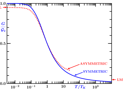
Figure 4: Thermal dependences of the conductance for two sets of model paramters, obtained from Eqs. (8) and (10). The solid line depicts the universal conductance curveCosti et al. (1994) for the symmetric Hamiltonian (11) . Here, it was computed with $\Gamma=0.1\,D$ and $U=3\,D$. The temperatures were scaled by the Kondo temperature $T_{K}=2.4\times 10^{-6}\,D/k_{B}$, fixed by the requirement $G(T_{K})=0.5{\mathcal{G}}_{2}$. The dashed curve is the conductance for the Hamiltonian (5) with $\Gamma=0.1\,D$, $U=3\,D$, $\varepsilon_{d}=-0.3\,D$, and $W=0$, which yielded $T_{K}=4.0\times 10^{-3}\,D$. To keep the data within the temperature range $k_{B}T<0.1\,D$, the dashed plot stops at $T=25\,T_{K}$. The horizontal arrows pointing to the vertical axes indicate the corresponding fixed-point conductances, given by Eqs. (22a) and (22b).

Particle-hole asymmetry drives $G$ away from $G^{S}$. For $U+2\epsilon_{d}\neq 0$ or $W\neq 0$, the universal curve $G^{S}(T/T_{K})$ no longer matches $G(T/T_{K})$. An example is the dashed curve in Fig. 4, calculated with $\Gamma=0.1\,D$, $U=3\,D$, $\varepsilon_{d}=-0.3\,D$, and $W=0$. The definition $G(T_{K})=0.5{\mathcal{G}}_{2}$, which in this case yields $T_{K}=4\times 10^{-3}\,D$, forces the solid and the dashed lines to agree at $T=T_{K}$; the conductance for the asymmetric model nonetheless undershoots (overshoots) the universal curve for $T<T_{K}$ ($T>T_{K}$). To reconcile this discrepancy with the concept of universality, the following sections rely on renormalization-group concepts.

IV Fixed points

Renormalization-goup theory probes the spectrum of Hamiltonians in search of characteristic energies and scaling invariances. The wire Hamiltonian (1), for instance, exhibits a single, trivial characteristic energy: the conduction bandwidth $2D$. For energies $\epsilon\ll D$, therefore, its spectrum is invariant under the scaling transformation $H_{w}\to\Lambda H_{w}$, for arbitrary scaling parameter $\Lambda>1$. Accordingly, for $\epsilon\ll D$, the wire Hamiltonian is a stable fixed point of the renormalization-group transformation in Ref. Krishna-murthy et al., 1980a.

Latent in the Anderson Hamiltonian (5), by contrast, are the four nontrivial characteristic energies discussed in Section II.3. Part of the spectrum of $H_{A}$ lies close to fixed points; the remainder is in transition ranges. In the vicinity of a fixed point, the spectrum remains approximately invariant under scaling; in the transition intervals, the eigenvalues are comparable to one or more characteristic energies and hence change rapidly under scale transformations. In particular, the portion of the spectrum pertinent to the Kondo regime comprises two lines of fixed points and a crossover region.

For given thermal or excitation energy $\mathcal{E}$, the inequality $\max(\mathcal{E},\Gamma_{W})\ll\min(|\varepsilon_{d}|,\varepsilon_{d}+U,D)$ defines the Kondo regime. As Fig. 3 shows, the dot occupation is then nearly unitary. In the energy range $k_{B}T_{K}\ll\mathcal{E}\ll\min(|\varepsilon_{d}|,\varepsilon_{d}+U,D)$, which is removed from characteristic energies, the Hamiltonian $H_{A}$ is near the Local Moment fixed point (LM). At very low energies, $\mathcal{E}\ll k_{B}T_{K}$, i. e., below the energy scale defined by the narrow set of levels at the center of Fig. 3, the spectrum becomes asymptotically invariant under scaling as the Hamiltonian approaches the Frozen Level fixed-point (FL). In the intermediate region $\mathcal{E}\sim k_{B}T_{K}$, the Hamiltonian crosses over from the LM to the FL.

IV.1 Fixed-point Hamiltonians

As the two central columns in Fig. 3 indicate, the LM is an unstable fixed-point consistent of a conduction band and a free spin-1/2 variable. In the FL, a singlet replaces the spin, and the Hamiltonian is equivalent to a conduction band—a stable fixed point. In their most general form, the fixed-point conduction bands mimic the wire Hamiltonian, i. e.,

$$H_{LM}^{*}=\sum_{k}\epsilon_{k}a_{k}^{\dagger}a_{k}+W_{LM}f_{0}^{\dagger}f_{0},$$ (14)

and

$$H_{FL}^{*}=\sum_{k}\epsilon_{k}a_{k}^{\dagger}a_{k}+W_{FL}f_{0}^{\dagger}f_{0},$$ (15)

with scattering potentials $W_{FL}$ and $W_{LM}$ dependent on $V$, $W$, $U$ and $\epsilon_{d}$. Equations (14) and (15) identify two lines of fixed points, parametrized by $W_{LM}$ and $W_{FL}$, respectively.

The Schrieffer-Wolff transformation offers an approximation for the LM potential:

$$\rho W_{LM}=\rho W+2\frac{\Gamma_{W}}{\pi|\varepsilon_{d}|}\frac{2\varepsilon_{d}+U}{\varepsilon_{d}+U}.$$ (16)

For most applications, this expression is insufficiently accurate, and an NRG computation is necessary to determine $W_{LM}$ and $W_{FL}$. The exception is the Hamiltonian (11), for which $W_{LM}=0$, as required by particle-hole symmetry.

IV.2 Fixed-point phase shifts

Appendix A diagonalizes the quadratic Hamiltonians (14) and (15). For the LM, the diagonal form reads

$$H_{LM}^{*}=\sum_{k}\varepsilon_{\ell}g_{\ell}^{\dagger}g_{\ell},$$ (17)

with phase-shifted energies

$$\varepsilon_{\ell}=\epsilon_{\ell}-\frac{\delta_{LM}}{\pi}\Delta.$$ (18)

At the LM, all conduction states are uniformly phase-shifted, with

$$\tan\delta_{LM}=-\pi\rho W_{LM}.$$ (19)

For $H_{A}=H_{A}^{S}$, in particular, $\delta_{LM}=0$, and the low-energy eigenvalues $\varepsilon_{k}$ coincide with the $\epsilon_{k}$.

The FL eigenvalues are likewise uniformly phase-shifted,

$$H_{FL}^{*}=\sum_{k}\tilde{\varepsilon}_{k}\tilde{g}_{k}^{\dagger}\tilde{g}_{k},$$ (20)

where $\tilde{\varepsilon}_{k}=\epsilon_{k}-(\delta/\pi)\Delta$. From the Friedel sum rule, it follows thatLangreth (1966)

$$\delta=\delta_{LM}-\frac{\pi}{2}.$$ (21)

For $H_{A}=H_{A}^{S}$, in particular, $\delta=\pi/2$.

IV.3 Conductance at the fixed points

The LM is the fixed point to which the Anderson Hamiltonian would come if $\Gamma=0$. For $0<\Gamma\ll\min(|\epsilon_{d}|,\epsilon_{d}+U,D)$, although the renormalization-group flow never reaches the LM, it brings $H_{A}$ close to the fixed point. The substantial portion of the spectrum of $H_{A}$ marked by the thin double-headed arrow in Fig. 3 is approximately described by the many-body eigenvalues of $H_{LM}^{*}$, and in the pertinent energy range, the physical properties of $H_{A}$ and $H_{LM}^{*}$ are approximately the same. Likewise, at low temperatures, the properties of $H_{A}$ approach those of $H_{FL}^{*}$.

The renormalization-group evolution of the Hamiltonian can be traced in the termal dependence of the conductance. As the temperature is reduced from $T\gg T_{K}$ to $T\ll T_{K}$, each curve in Fig. 4 crosses over from a lower plateau to a higher one. The extension of Langreth’s expression Langreth (1966) derived in Appendix B determines the plateau conductances:

$$G_{LM} = {\mathcal{G}}_{2}\sin^{2}(\delta_{LM}-\delta_{W})={\mathcal{G}}_{2}\cos^{2}(\delta-\delta_{W});\quad$$ (22a)

$$G_{FL} = {\mathcal{G}}_{2}\sin^{2}(\delta-\delta_{W}),$$ (22b)

where $\delta_{W}$ is the ground-state phase shift for $V=0$. According to the analysis in Appendix A,

$$\tan\delta_{W}=-\pi\rho W.$$ (23)

The solid curve in Fig 4 was computed for $H_{A}=H_{A}^{S}$, so that $\delta_{W}=0$, while the ground-state (i. e., FL) phase shift is $\delta=\pi/2$. According to Eqs. (22), $G_{LM}=0$ and $G_{FL}={\mathcal{G}}_{2}$, in agreement with the plot. The ground-state phase shift for the dashed curve, extracted from the low-energy eigenvalues in the NRG run that generated it, is somewhat lower: $\delta=0.43\pi$. Again $\delta_{W}=0$, and the two horizontal arrows pointing to the vertical axes in Fig. 4 indicate the conductances predicted by Eqs. (22). Given the relatively high Kondo temperature ($k_{B}T_{K}=4\times 10^{-3}\,D$) in this run, the condition $k_{B}T\ll D$ restricts the curve to the range $T<25\,T_{K}$, so that, even at the highest temperature shown, $H_{A}$ is relatively distant from the LM, and Eq. (22a) cannot be accurately checked. At low temperatures, however, the renormalization-group flow bringing $H_{A}$ asymptotically close to $H_{FL}^{*}$, the agreement with Eq. (22b) is excellent.

V Crossover

In the Kondo regime, the Schrieffer-Wolff transformationSchrieffer and Wolff (1966) brings the Anderson Hamiltonian $H_{A}$ to the Kondo form

$$H_{J}=\sum_{k}\epsilon_{k}a_{k}^{\dagger}a_{k}+W_{LM}f_{0}^{\dagger}f_{0}+J\sum_{\mu\nu}f_{0\mu}^{\dagger}\bm{\sigma}_{\mu\nu}f_{0\nu}\cdot\bm{S},$$ (24)

with $J$ defined in Eq. (13).

To eliminate the scattering potential on the right-hand side, it is convenient to project $H_{J}$ upon the basis of the eigenoperators $g_{k}$ of the LM, which yieldsirr

$$H_{J}=\sum_{k}\varepsilon_{\ell}g_{\ell}^{\dagger}g_{\ell}+J_{W}\sum_{\mu\nu}\phi_{0\mu}^{\dagger}\bm{\sigma}_{\mu\nu}\phi_{0\nu}\cdot\bm{S},$$ (25)

where $J_{W}=J\cos^{2}\delta_{LM}$, and

$$\phi_{0}=\frac{1}{\sqrt{N}}\sum_{\ell}g_{\ell}.$$ (26)

In the symmetric case $\delta_{LM}$ vanishes, and the operator $\phi_{0}$ reduces to $f_{0}$.

The second term on the right-hand side of Eq. (25) drives the Hamiltonian from the LM to the FL. Along the resulting trajectory, the eigenvalues of $H_{J}$ scale with $T_{K}$.Wilson (1975); Krishna-murthy et al. (1980b); Tsvelick and Wiegmann (1983); Andrei et al. (1983) Let $T_{K}$ and $\bar{T}_{K}<T_{K}$ be the Kondo temperatures correspondig to two sets of model parameters in the Kondo regime: $\mathcal{M}\equiv\left\{\Gamma,W,U,\varepsilon_{d}\right\}$ and $\bar{\mathcal{M}}\equiv\left\{\bar{\Gamma},\bar{W},\bar{U},\bar{\varepsilon}_{d}\right\}$, to which correspond the antiferromagnetic couplings $J$ and $\bar{J}$, respectively. If $|m\rangle$ is an eigenvector of $H_{J}$ with eigenvalue $E_{m}$, then a corresponding eigenvector $|\bar{m}\rangle$ of $H_{\bar{J}}$, the scaling image of $|m\rangle$, can always be found, with the same quantum numbers and eigenvalue $\bar{E}_{m}$ such that $E_{m}/T_{K}=\bar{E}_{m}/\bar{T}_{K}$.

The matrix elements of any linear combination of the operators $g_{k}$ are moreover universal. Given two eigenstates $|m\rangle$ and $|n\rangle$ of $H_{J}$ and their scaling images $|\bar{m}\rangle$ and $|\bar{n}\rangle$, then the matrix elements of $\phi_{0}$, for example, are equal: $\langle m|\,\phi_{0}\,|n\rangle=\langle\bar{m}|\,\phi_{0}\,|\bar{n}\rangle$. Likewise, the matrix elements of the operator

$$\phi_{1}=\sqrt{\frac{3}{N}}\sum_{\ell}\frac{\varepsilon_{\ell}}{D}g_{\ell}$$ (27)

are universal: $\langle m|\,\phi_{1}\,|n\rangle=\langle\bar{m}|\,\phi_{1}\,|\bar{n}\rangle$.

V.1 Thermal dependence of the conductance

By contrast, the matrix elements $\langle m|\,c_{d}\,|n\rangle$ on the right-hand side of Eq. (10) are non-universal. Even at the lowest energies, as Eq. (79) shows, they depends explicitly on the model parameters. To discuss universal properties, therefore, we must relate them to universal matrix elements, such as $\langle m|\,\phi_{0}\,|n\rangle$, $\langle m|\,\phi_{1}\,|n\rangle$, or $\langle m|\,g_{\ell}\,|n\rangle$. As a first step towards that goal, we evaluate the commutator

$$[H_{A},a_{q}^{\dagger}]=\epsilon_{q}a_{q}^{\dagger}+\frac{V}{\sqrt{N}}c_{d}^{\dagger}+\frac{W}{N}\sum_{p}a_{p}^{\dagger},$$ (28)

and sum the result over $q$, to find that

$$[H_{A},f_{0}^{\dagger}]=\frac{1}{\sqrt{3}}f_{1}^{\dagger}+Vc_{d}^{\dagger}+Wf_{0}^{\dagger}.$$ (29)

Here we have defined another shorthand

$$f_{1}=\sqrt{\frac{3}{N}}\sum_{q}\frac{\epsilon_{q}}{D}\,a_{q}.$$ (30)

Equation (29) relates the matrix elements of $c_{d}^{\dagger}$ between two (low energy) eigenstates $|m\rangle$ and $|n\rangle$ of $H_{A}$ to those of the operators $f_{0}$ and $f_{1}$:

$$V\langle m|\,c_{d}^{\dagger}\,|n\rangle=(E_{m}-E_{n}-W)\langle m|\,f_{0}^{\dagger}\,|n\rangle-\sqrt{3}D\langle m|\,f_{1}^{\dagger}\,|n\rangle.$$ (31)

In the Kondo regime, with $\max(E_{m},E_{n})\ll D$, the first two terms within the parentheses on the right-hand side can be dropped.

In the symmetric case, since $f_{0}$ ($f_{1}$) coincides with $\phi_{0}$ ($\phi_{1}$), Eq. (31) shows that the product $V\langle m|\,c_{d}\,|n\rangle$ is universal, in line with the firmly established notion that $\Gamma\rho_{d}(\epsilon/k_{B}T_{K},T/T_{K})$, and $G^{S}(T/T_{K})$ are universal functions.Costi et al. (1994); Bulla et al. (2008) To discuss asymmetric Hamiltonians, we have to relate the operators $f_{0}$ and $f_{1}$ to $\phi_{0}$ and $\phi_{1}$. This is done in Appendix A.2, which shows that, in the Kondo regime, a linear transformation with model-parameter dependent coefficients relates the matrix elements of both $f_{0}$ and $f_{1}$ to those of $\phi_{0}$ and $\phi_{1}$. When Eq. (67) is substituted for $f_{0}$ and $f_{1}$ on the right-side of Eq. (31), it results that

$$\sqrt{\pi\rho\Gamma_{W}}\langle m|\,c_{d}^{\dagger}\,|n\rangle=\alpha_{0}\langle m|\,\phi_{0}^{\dagger}\,|n\rangle+\alpha_{1}\langle m|\,\phi_{1}^{\dagger}\,|n\rangle.$$ (32)

Here, the constants $\alpha_{0}$ and $\alpha_{1}$ are combinations of the (unknown) linear coefficients on the right-hand side of Eq. (67), the parameter $W$ on the right-hand side of Eq. (31), and the ratio $\sqrt{\pi\rho\Gamma_{W}}/V$, by which we multiplied Eq. (31) to shorten the following algebra.

Substitution in Eq. (10) yields an expression relating the spectral density $\rho_{d}$ to universal functions:

$$\pi\rho\Gamma_{W}\rho_{d}(\epsilon,T)=\alpha_{0}^{2}\rho_{0}(\epsilon,T)+\alpha_{1}^{2}\rho_{1}(\epsilon,T)+\alpha_{0}\alpha_{1}\rho_{(01)}(\epsilon,T),$$ (33)

where

$$\rho_{j}\,(\epsilon,T) =\displaystyle\sum_{mn} \frac{e^{-\beta E_{m}}}{\mathcal{Z}f(\epsilon)}|\langle n|\,\phi_{j}\,|m\rangle|^{2}$$ (34)

$$\times\,\delta(E_{m}-E_{n}-\epsilon)\qquad(j=0,1),$$

and

$$\rho_{(01)}\,(\epsilon,T) =\displaystyle\sum_{mn} \frac{e^{-\beta E_{m}}}{\mathcal{Z}f(\epsilon)}\,\left(\langle m|\,\phi_{0}^{\dagger}\,|n\rangle\langle n|\,\phi_{1}\,|m\rangle+\text{c.~{}c.}\right)$$ (35)

$$\times\,\delta(E_{m}-E_{n}-\epsilon).$$

Next, we substitute Eq. (33) on the right-hand side of Eq. (8), to split the conduction into three pieces:

$$G(T)=\alpha_{0}^{2}G_{0}(T)+\alpha_{1}^{2}G_{1}(T)+\alpha_{0}\alpha_{1}G_{(01)}(T),$$ (36)

where

$$G_{j}(T)=\frac{{\mathcal{G}}_{2}}{\rho}\,\int_{-D}^{D}\rho_{j}(\epsilon,T)\left[-\frac{\partial f(\epsilon)}{\partial\epsilon}\right]\,d\epsilon\qquad(j=0,1),$$ (37)

and

$$G_{(01)}(T)=\frac{{\mathcal{G}}_{2}}{\rho}\int_{-D}^{D}\rho_{(01)}(\epsilon,T)\left[-\frac{\partial f(\epsilon)}{\partial\epsilon}\right]\,d\epsilon.$$ (38)

V.2 Universal contributions to the conductance

Given the universality of the energies $E_{m}$ and of the matrix elements $\langle m|\,\phi_{j}\,|n\rangle$ ($j=1,2$) on the right-hand sides of Eqs. (34) and (35), we see that the spectral densities $\rho_{j}(\epsilon,T)$ ($j=0,1$), and $\rho_{(01)}(\epsilon,T)$ are universal. Inspection of the right-hand sides of Eqs. (37-38) shows that the functions $G_{j}$ ($j=0,1$) and $G_{(01)}$ are likewise universal. To compute them, we are free to consider any convenient Kondo-regime Hamiltonian.

Particle-hole symmetry makes $H_{A}^{S}$ especially convenient. To show that the cross terms make no contribution to the conductance, i. e., that $G_{(01)}(T)=0$, we only have to notice that, while leaving $H_{A}^{S}$ unchanged, the particle-hole transformation $c_{d}\to-c_{d}^{\dagger}$, $g_{k}\to g_{k}^{\dagger}$ (i. e., $a_{k}\to a_{k}^{\dagger}$) reverses the sign of the product of matrix elements $\langle m|\,\phi_{i}^{\dagger}\,|n\rangle\langle n|\,\phi_{j}\,|m\rangle+\text{c.~{}c.}$ on the right-hand side of Eq. (35). We see that $\rho^{(01)}(\epsilon,T)$ is an odd function of $\epsilon$, so that the integral on the right-hand side of Eqs (38) vanishes.

To evaluate $G_{0}$ and $G_{1}$, we start out from the closed form resulting from the diagrammatic expansion (in the coupling $V$) of the conduction-electron retarded Green’s function for the symmetric Hamiltonian:

$$\mathbb{G}_{kk^{\prime}}^{S}(\epsilon)=\mathbb{G}^{(0)}_{k}(\epsilon)\delta_{kk^{\prime}}+\frac{V^{2}}{N}\mathbb{G}^{(0)}_{k}(\epsilon)\mathbb{G}_{d}^{S}(\epsilon)\mathbb{G}^{(0)}_{k^{\prime}},$$ (39)

where $\mathbb{G}_{d}^{S}$ is the retarded dot-level Green’s function for the symmetric Hamiltonian, and

$$\mathbb{G}^{(0)}_{k}(\epsilon)=\frac{1}{\epsilon-\epsilon_{k}+i\eta}$$ (40)

is the free conduction-electron retarded Green’s function.

From $\mathbb{G}_{kk^{\prime}}^{S}$, it is a simple matter to obtain the spectral densities on the right-hand side of Eq. (33):

$$\rho_{0}(\epsilon,T)=-\frac{1}{\pi N}\Im\sum_{kk^{\prime}}\mathbb{G}_{kk^{\prime}}^{S}(\epsilon),$$ (41)

and

$$\rho_{1}(\epsilon,T)=-\frac{3}{\pi ND^{2}}\Im\sum_{kk^{\prime}}\epsilon_{k}\epsilon_{k^{\prime}}\mathbb{G}_{kk^{\prime}}^{S}(\epsilon).$$ (42)

To compute the conductances at temperatures $T$ satisfying $k_{B}T\ll D$, we only need the spectral densities for $\epsilon\ll D$. It is appropriate, therefore, to expand the right-hand side of Eq. (40) to linear order in $\epsilon/D$:

$$\mathbb{G}^{(0)}_{k}(\epsilon)=\frac{2\epsilon}{D}-i\pi\delta(\epsilon-\epsilon_{k})\qquad(\epsilon\ll D).$$ (43)

The sums over momenta on the right-hand side of Eqs. (41) and (42) are then easily computed. Among the resulting terms, only the even powers of $\epsilon$ contribute to the integral on the right-hand side of Eq. (37). To compute the conductance to $\mathcal{O}[(k_{B}T/D)^{2}]$ we hence neglect the terms of $\mathcal{O}(\epsilon/D)$. Equation (41) then gives

$$\rho_{0}(\epsilon,T)=\rho-{\pi\rho\Gamma}\rho_{d}^{S}(\epsilon,T),$$ (44)

equivalent to an expression obtained in Ref.Maruyama et al. (2004).

Substitution of this result for $\rho_{0}$ on the right-hand side of Eq. (37) establishes a simple relation between the universal function $G_{0}$ and the universal conduction for the symmetric Hamiltonian:

$$G_{0}(T)={\mathcal{G}}_{2}-G^{S}(T).$$ (45)

Equation (45) becomes exact, asymptotically, at low temperatures. The deviations, of $\mathcal{O}[(k_{B}T/D)^{2}]$, are insifignicant. As an illustration, the open circles in Fig. 5 show NRG data for the conductance $G_{0}(T)$, Eq. (37), in excellent agreement with the solid line representing the right-hand side of Eq. (45).

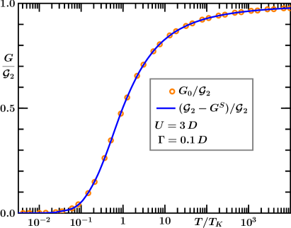
Figure 5: NRG results for the thermal dependence of the auxiliary conductance $G_{0}(T)$, associated with the spectral density for the operator $\phi_{0}$. The open circles show Eq. (37) for $j=0$, computed for the symmetric Hamiltonian with the displayed model parameters. The solid line is the right-hand side of Eq. (45), i. e., the universal curve in Fig. 4 subtracted from the quantum conductance ${\mathcal{G}}_{2}$.

To the same accuracy, we can neglect the $\mathcal{O}(\epsilon/D)$ terms resulting from the summation on the right-hand side of Eq. (42), which yields

$$\rho_{1}(\epsilon,T)=\frac{6\rho\Gamma}{\pi}\rho_{d}^{S}(\epsilon,T).$$ (46)

Equation (37) then shows that $G_{1}$ is also related to the conductance for the symmetric Hamiltonian:

$$G_{1}(T)=\frac{6}{\pi^{2}}G^{S}(T),$$ (47)

V.3 Mapping to the universal conductance

The combination of Eqs. (45) and (47) with the result $G_{(01)}=0$ reduces Eq. (36) to the equality

$$G(T)=\alpha_{0}^{2}\bm{\left(}{\mathcal{G}}_{2}-G^{S}(T)\bm{}+\alpha_{1}^{2}\,\frac{6}{\pi}\,\rho\,G^{S}(T)$$ (48)

To determine the coefficients $\alpha_{0}$ and $\alpha_{1}$, we need only compare the right-hand side with the fixed-point expressions for the conductance. At the LM, $G^{S}=0$, and Eq. (22a) shows that $\alpha_{0}^{2}=\cos^{2}(\delta-\delta_{W})$. At the FL, $G^{S}={\mathcal{G}}_{2}$, and Eq. (22b) shows that $(6/{\pi}^{2})\alpha_{1}^{2}=\sin^{2}(\delta-\delta_{W})$. These two results turn Eq. (48) into the mapping

$$G\bm{\left(}\frac{T}{T_{K}}\bm{}-\frac{{\mathcal{G}}_{2}}{2}=-\bm{\left(}G^{S}\bm{\left(}\frac{T}{T_{K}}\bm{}-\frac{{\mathcal{G}}_{2}}{2}\bm{}\cos 2(\delta-\delta_{W}).$$ (49)

V.4 Illustrative numerical results

Equation (12) offers an approximation for $T_{K}$, and Eqs. (16), (19) and (21) provide an approximation for the ground-state phase shift $\delta$. These estimates are far from the accuracy needed to fit numerical or experimental data. In the laboratory, $T_{K}$ and $\delta-\delta_{W}$ are adjustable parameters; the former, in particular, is determined by the condition $G(T_{K})={\mathcal{G}}_{2}/2$.Goldhaber-Gordon et al. (1998c); Katsumoto et al. (2006); Sato et al. (2005) In the computer office, the two unknown parameters on the right-hand side of Eq. (49) can can be extracted from the conductance itself, or from other properties of the model Hamiltonian. The phase shift $\delta$ is most easily obtained from the ground-state eigenvalues of $H_{A}$. To determine the Kondo temperature $T_{K}$, it has been traditional to fit the thermal dependence of the magnetic susceptibility $\chi(T)$ with the universal curve for $k_{B}T\chi(T/T_{K}).$Krishna-murthy et al. (1980a); Tsvelick and Wiegmann (1983) Here, however, we prefer the laboratory definition, which insures that both sides of Eq. (49) vanish at $T=T_{K}$.

Figure 6 displays the results of two NRG runs for the same assymetric parameters $U=3\,D$, $\epsilon=-0.3\,D$, $\Gamma=0.1\,D$, with two scattering potentials $W=0$ and $W=-0.6\,D$. The open circles reproduce the dashed curve in Fig. 4. The particle-hole asymmetry, combined with the relatively high ratio between the dot width and excitation energy, $\Gamma/|\epsilon|=1/3$, place the model Hamiltonian close to the border of the Kondo domain. Although $W=0$, the ground-state phase shift deviates significantly from $\pi/2$: from the FL eigenvalues generated by the NRG diagonalization of the model Hamiltonian, we find $\delta=0.43\pi$. The solid curve through the center of the circles is a plot of Eq. (49) with $\delta-\delta_{W}=0.43\pi$ and $k_{B}T_{K}=4\times 10^{-3}\,D$.

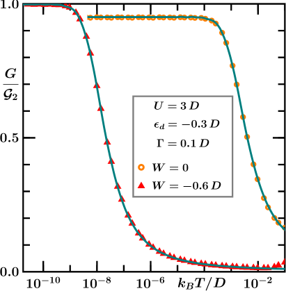
Figure 6: Numerical data for the temperature dependence of the conductance, compared to Eq. (49). The open circles and triangles show the NRG computed conductances for the indicated model parameters. The solid lines represent the mapping , with ground-phase shifts calculated from the FL eigenvalues of the model Hamiltonian and $T_{K}$ determined by the condition $G(T_{K})={\mathcal{G}}_{2}/2$. The small disagreement between the triangles and the solid line above $k_{B}T=10^{-2}\,D$ is due to the relatively large irrelevant operators introduced by the scattering potential $W$, whose contribution to $G$ decays in proportion to $k_{B}T/D$.

The scattering potential $W=-0.6\,D$ reduces the Kondo temperature and raises the FL conductance $G(T=0)$. The former shrinks to $k_{B}T_{K}=2.2\times 10^{-8}\,D$, while the latter rises to nearly ${\mathcal{G}}_{2}$. Both changes are due to the reduced dot width $\Gamma_{W}=\cos\delta_{W}\Gamma$. Here Eq. (9) yields $\rho\Gamma_{W}=0.74\rho\Gamma=0.074$, and the resulting smaller antiferromagnetic coupling (13) brings the Kondo temperature (12) down five orders of magnitude.

The diminished Kondo temperature indicates that the scattering potential has pushed the model Hamiltonian deeper inside the Kondo regime. Other indications are the minute high-temperature conductance; the nearly ballistic low-temperature conductance; and the overall similarity between $G(T/T_{K})$ and the solid line in Fig. 4.

V.5 Discussion

In the Kondo regime, Eqs. (22a) and (22b) fix the high- and the low-temperature conductances, respectively. Equation (49) shows that the universal function $G^{S}(T/T_{K})$ controls the monotonic transition between the two limits. For $W=0$, in particular, the fixed-point values depend only on the ground-state phase shift $\delta$ and are symmetric with respect to ${\mathcal{G}}_{2}/2$: $G_{LM}={\mathcal{G}}_{2}\cos^{2}\delta$ and $G_{FL}={\mathcal{G}}_{2}\sin^{2}\delta$. Thus, depending on $\delta$, the transition from $G_{LM}$ to $G_{FL}$ can be steeper or flatter. Since $\delta$ can never depart much from $\pi/2$ in the Kondo regime, the argument of the trigonometric function on the right-hand side of Eq. (49) can never depart substantially from $\pi$, and as indicated by the two curves in Fig. 4, $G(T/T_{K})\approx G^{S}(T/T_{K})\pm 20\%$. By contrast with this crude estimate, the mapping (49) gives excellent agreement with the circles in Fig. 6.

The wire potential $W$ narrows the dot level and displaces the ground-state phase shift. Depending on the sign and magnitude of $W$, the phase shift can take any value in its domain of definition $-\pi/2\leq\delta\leq\pi/2$. In the Kondo regime, the Friedel sum rule nonetheless prevents the difference $\delta-\delta_{W}$ from straying away from $\pi/2$. All effects considered, the scattering potential $W$ displaces the conductance curve towards the symmetric limit $G(T/T_{K})=G^{S}(T/T_{K})$.

These findings are in line with the experimentally established notion that, in the Kondo regime, SET conductances always decay with temperature.Goldhaber-Gordon et al. (1998a, b); van der Wiel et al. (2000); Liang et al. (2002) A brief comparison between this behavior and that of the side-coupled device Kobayashi et al. (2004); Sato et al. (2005) seems appropriate. As demonstrated in Ref. Seridonio et al., 2007, a linear mapping analogous to Eq. (49) can be established between the side-coupled conductance and $G^{S}(T/T_{K})$; in that case, however, the coefficient relating the two functions is independent of $\delta_{W}$ and hence free from the constraint imposed by the Friedel sum rule. Under a sufficiently strong wire potential, its sign can be reversed. Thus, the thermal dependence of $G_{SC}$ is tunable:Katsumoto (2007) a wire potential can turn a monotonically increasing function into a monotonically decreasing one. The embedded geometry of Fig. 1 is much less sensitive to $W$.

The parameter $\delta_{W}$ is ($\pi$ times) the charge induced under the wire electrodes by the potential $W$. According to the Friedel sum rule, Langreth (1966) the difference $\delta-\delta_{W}$ is the charge of the Kondo cloud, the additional charge that piles up at the wire tips surrounding the dot as the temperature is lowered past $T_{K}$. Neutrality makes the charge of the Kondo cloud equal to the dot occupancy. Since the symmetric condition $n_{d}=1$ maximizes the the low-temperature conductance, one expects $G(T=0)$ to be ballistic for $2(\delta-\delta_{W})=\pi$, a conclusion in agreement with Eq. (49). Since the screening charge is always nearly unitary, one expects the low-temperature conductance to be close to the conductance quantum, in agreement with the plots in Fig. 6.

VI Conclusions

Our central result, Eq. (49) maps the conductance in the embedded geometry onto the universal conductance for the symmetric Anderson model (11). Different from the universal result for the side-coupled geometry, the mapping depends explicitly on the potential $W$ applied to the wire. Section V showed that, in the Kondo regime, the Friedel sum rule anchors the the argument of the cosine on the right-hand side of Eq. (49) to the vicinity of $\pi$; it results that $G(T/T_{K})$ reproduces semiquantitatively the universal function $G^{S}(T/T_{K})$.

At the quantitative level, Eq. (49) affords comparison with experimental data collected anywhere in the Kondo regime. For that purpose, its linearity is particularly convenient. Once fitted to a set of experimental points, the mapping determines the Kondo temperature $T_{K}$, as well as the phase shift difference $\delta-\delta_{W}$. Both are quantities of physical significance. According to the Friedel sum rule, the phase shift difference is ($\pi/2$ times) the screening charge surrounding the dot at low temperatures.

In summary, we have derived an exact expression relating the SET conductance in the Kondo regime to the universal conductance function for the symmetric Anderson Hamiltonian. A subsequent report will exploit this result in an attempt to offer a unified view of an NRG survey of conductance in the Kondo regime.

Appendix A Properties of the fixed-point Hamiltonians

A.1 Diagonalization

The LM and FL are described by conduction-band Hamiltonians of the form

$$H^{*}=\sum_{k}\epsilon_{k}a_{k}^{\dagger}a_{k}+W^{*}f_{0}^{\dagger}f_{0}.$$ (50)

We want to bring $H^{*}$ to the diagonal form

$$H^{*}=\sum_{\ell}\varepsilon_{\ell}g_{\ell}^{\dagger}g_{\ell},$$ (51)

where

$$g_{\ell}=\sum_{q}\alpha_{\ell q}a_{q}.$$ (52)

To this end, we compare the expressions for the commutator $[g_{\ell},H^{*}]$ obtained from Eqs. (50) and (51), from which it follows that

$$\alpha_{\ell q}=\frac{1}{\varepsilon_{\ell}-\epsilon_{q}}\frac{W^{*}}{N}\sum_{k}\alpha_{\ell k}.$$ (53)

Summation of both sides over $q$ then leads to the eigenvalue condition:

$$1=\frac{W^{*}}{N}\sum_{q}\frac{1}{\varepsilon_{\ell}-\epsilon_{q}}.$$ (54)

Inspection of this equality shows that, with exception of a split-off energy, which makes $\mathcal{O}(1/N)$ contributions to the low-energy properties, the $\varepsilon_{\ell}$ are shifted by less than $\Delta$ from the $\epsilon_{k}$. We therefore refer to the closest conduction energy $\epsilon_{\ell}$ to label each eigenvalue and define its phase shift $\delta_{\ell}$ with the expression

$$\varepsilon_{\ell}\equiv\epsilon_{\ell}-\frac{\Delta}{\pi}\delta_{\ell}.$$ (55)

This definition substituted in Eq. (54), a Sommerfeld-Watson transformationMatthews and Walker (1971) determines the sum on the right-hand side:

$$\frac{1}{N}\sum_{q}\frac{1}{\varepsilon_{\ell}-\epsilon_{q}}=-\pi\rho\cot\delta_{\ell}+\rho\,\fint_{-D}^{D}\frac{1}{\varepsilon_{\ell}-\epsilon}\,d\epsilon.$$ (56)

Substitution in Eq. (54) results in an expression for the phase shifts:

$$\cot\delta_{\ell}=-\frac{1}{\pi\rho W^{*}}+\frac{1}{\pi}\,\fint_{-D}^{D}\frac{1}{\varepsilon_{\ell}-\epsilon}\,d\epsilon.$$ (57)

At low energies, the contribution of the last term on the right-hand side, of $\mathcal{O}(\epsilon/D)$, can be neglected, which shows that the phase shift becomes uniform:

$$\tan\delta=-\pi\rho W^{*}.$$ (58)

To determine the coefficients $\alpha_{\ell q}$, we square both sides of Eq. (53) and sum the result over $q$:

$$\sum_{q}\alpha^{2}_{\ell q}=\bm{\left(}\sum_{k}\alpha_{\ell k}\frac{W^{*}}{N}\bm{}^{2}\sum_{q}\frac{1}{(\varepsilon_{\ell}-\epsilon_{q})^{2}}.$$ (59)

To evaluate the sum on the left-hand side, we differentiate Eq. (56) with respect to $\epsilon_{\ell}$, which yields, with relative error $\mathcal{O}(1/N)$,

$$\frac{1}{N^{2}}\sum_{q}\frac{1}{(\varepsilon_{\ell}-\epsilon_{q})^{2}}=\bm{\left(}\frac{\pi\rho}{\sin\delta_{\ell}}\bm{}^{2}.$$ (60)

The sum on the left-hand side of Eq. (59) being unitary, Eq. (60) shows that

$$W^{*}\sum_{k}\alpha_{\ell k}=-\frac{1}{\pi\rho}\sin\delta_{\ell},$$ (61)

the negative phase insuring that $\alpha_{kk}\to 1$ for $W^{*}\to 0$. Equation (53) then gives

$$\alpha_{\ell q}=\frac{\Delta}{\epsilon_{q}-\varepsilon_{\ell}}\frac{\sin\delta_{\ell}}{\pi}\qquad(\varepsilon_{\ell}\ll D).$$ (62)

A.2 Energy moments of the matrix elements of the eigenoperators $g_{\ell}$

The Hamiltonian (50) diagonalized, we turn our attention to the following energy moments

$$M_{mn}^{\,(p)}\equiv\frac{1}{\sqrt{N}}\sum_{\ell}\bm{\left(}\frac{\varepsilon_{\ell}}{D}\bm{}^{p}\langle m|\,g_{\ell}\,|n\rangle\qquad(p=0,1,\ldots).$$ (63)

Chiefly important are $M_{mn}^{\,(0)}\equiv\langle m|\,\phi_{0}\,|n\rangle$ and $M_{mn}^{\,(1)}\equiv\langle m|\,\phi_{1}\,|n\rangle/\sqrt{3}$; the other moments, as shown below, are proportional to $M_{mn}^{\,(1)}\equiv\langle m|\,\phi_{1}\,|n\rangle$. Since the $M_{mn}^{p}$ are universal, to evaluate them it is sufficient to consider the symmetric Hamiltonian (11), for which the phase shift $\delta_{LM}=0$, so that $g_{k}$, $\varepsilon_{k}$, $\phi_{0}$, and $\phi_{1}$ coincide with $a_{k}$, $\epsilon_{k}$, $f_{0}$, and $f_{1}$, respectively.

From Eq. (11), we then have that

$$[g_{\ell},H_{A}^{S}]=\varepsilon_{\ell}g_{\ell}+\frac{V}{\sqrt{N}}c_{d}.$$ (64)

With the shortand $\mathcal{E}_{mn}\equiv(E_{m}-E_{n})/D$, the multiplication of both sides by $(\varepsilon_{\ell}/D)^{p-1}$ followed by summation over $\ell$ leads to the coupled recursive relations

$$\begin{array}[]{lll}M_{mn}^{\,(p)}=&-\mathcal{E}_{mn}M_{mn}^{\,(p-1)}-\displaystyle\frac{V}{p}\langle m|\,c_{d}\,|n\rangle&\qquad(p=1,3,\ldots);\\ M_{mn}^{\,(p)}=&-\mathcal{E}_{mn}M_{mn}^{\,(p-1)}&\qquad(p=2,4,\ldots).\end{array}$$

Reduced to a matrix equation, this system is easily solved. The result is

$$M_{mn}^{\,(p)}=\left\{\begin{array}[]{ll}M_{mn}^{\,(0)}\mathcal{E}_{mn}^{p}-\displaystyle\frac{V}{p}\langle m|\,c_{d}\,|n\rangle\bm{\left(}1+{\displaystyle\sum_{r=1}^{p-1}}\mbox{\raisebox{7.0pt}{$\prime$}}\frac{{\mathcal{E}_{mn}}^{r}}{r}\bm{}&\quad(p=\mathrm{odd})\\ M_{mn}^{\,(0)}\mathcal{E}_{mn}^{p}-\displaystyle\frac{V}{p}\langle m|\,c_{d}\,|n\rangle{\displaystyle\sum_{r=1}^{p-1}}\mbox{\raisebox{7.0pt}{$\prime$}}\frac{{\mathcal{E}_{mn}}^{r}}{r}&\quad(p=\mathrm{even})\end{array}\right.,$$

where the primed sum is restricted to odd $r$’s.

The pertinent energies satisfy the condition $k_{B}T\ll D$, which implies $\mathcal{E}_{mn}\ll 1$. It is therefore safe to discard the terms proportional to $\mathcal{E}_{mn}$ and its powers. Within this approximation, the only nonzero even moment is $M_{mn}^{\,(0)}$, and all odd moments are proportional to $\langle m|\,c_{d}\,|n\rangle$. It follows that all the odd moments are proportional to $M_{mn}^{\,(1)}=\langle m|\,\phi_{1}\,|n\rangle$:

$$M_{mn}^{\,(p)}=\left\{\begin{array}[]{ll}\displaystyle\frac{\langle m|\,\phi_{1}\,|n\rangle}{p}&\qquad(p=\text{odd})\\ 0&\qquad(p=2,4,\ldots)\end{array}\right..$$ (65)

An orthonormal basis describing the conduction band (51) can be constructed from the definition

$$\phi_{p}\equiv\sqrt{\frac{2p+1}{N}}\sum_{\ell}P_{p}(\epsilon_{\ell})g_{\ell}\qquad(p=0,1,\ldots),$$ (66)

where $P_{p}(\epsilon)$ denotes a Legendre polynomial.

According to Eq. (65), $\langle m|\,\phi_{p}\,|n\rangle\sim\langle m|\,\phi_{1}\,|n\rangle$ ($p=3,5,\ldots$), while $\langle m|\,\phi_{p}\,|n\rangle=0$ ($p=2,4,\ldots$). This shows that the matrix element of any conduction operator is a linear combination of $\langle m|\,\phi_{0}\,|n\rangle$ and $\langle m|\,\phi_{1}\,|n\rangle$. In particular

$$\langle m|\,f_{i}\,|n\rangle=\sum_{j=0}^{1}\alpha_{ij}\langle m|\,\phi_{j}\,|n\rangle\qquad(i=0,1),$$ (67)

where $f_{0}$ and $f_{1}$ are the operators defined by Eqs. (6) and (30), respectively, and the $\alpha_{ij}$ ($i,j=0,1$) are constants that depend on the model parameters.

Appendix B Fixed-point conductances

This appendix derives an expression for the spectral density $\rho_{d}(\epsilon,T)$, defined by Eq. (10), at the fixed points. The procedure is analogous to the one in Appendix A.

From Eq. (28) we obtain an expression for the matrix element of $a_{q}$ between two low-energy eigenstates $|m\rangle$ and $|n\rangle$ of eigenstates of $H_{A}$:

$$\langle m|\,a_{q}^{\dagger}\,|n\rangle = \frac{1}{\sqrt{N}}\frac{V}{E_{m}-E_{n}-\epsilon_{q}}\langle m|\,c_{d}^{\dagger}\,|n\rangle$$ (68)

$$+\frac{W}{N}\frac{1}{E_{m}-E_{n}-\epsilon_{q}}\langle m|\,\sum_{p}a_{p}^{\dagger}\,|n\rangle.$$

Summation of both sides over $q$ leads to an expression for the matrix element in the last term on the right-hand side:

$$\langle m|\,\sum_{p}a_{p}^{\dagger}\,|n\rangle\bm{\left(}1-W\mathcal{S}_{mn}\bm{}=\sqrt{N}V\langle m|\,c_{d}^{\dagger}\,|n\rangle\mathcal{S}_{mn},$$ (69)

where

$$\mathcal{S}_{mn}\equiv\frac{1}{N}\sum_{q}\frac{1}{E_{m}-E_{n}-\epsilon_{q}},$$ (70)

which brings Eq. (68) to the form

$$\langle m|\,a_{q}^{\dagger}\,|n\rangle=\frac{\langle m|\,c_{d}^{\dagger}\,|n\rangle}{\sqrt{N}(E_{m}-E_{n}-\epsilon_{q})}\frac{V}{1-W\mathcal{S}_{mn}}.$$ (71)

Consider now this equality at one of the two fixed points, LM or FL. The fixed-point Hamiltonian has then the quadratic form (51), which defines the complete basis of the operators $g_{\ell}$. The matrix element $\langle m|\,g_{\ell}^{\dagger}\,|n\rangle$ vanishes unless $|m\rangle=g_{\ell}^{\dagger}|n\rangle$, which implies $E_{m}=E_{n}+\varepsilon_{\ell}$. At a fixed point, therefore, the sum on the right-hand side of Eq. (70) reduces to that in Eq. (56), i. e.,

$$\mathcal{S}_{mn}=-\pi\rho\cot\delta_{*},$$ (72)

where we have disconsidered the last term on the right-hand side of Eq. (56) because at a fixed point the ratio $\varepsilon_{\ell}/D\to 0$. This result suggests that we introduce the phase shift $\delta_{W}$, defined by

$${W}\equiv-\frac{\tan\delta_{W}}{\pi\rho},$$ (73)

to simplify Eq. (71):

$$\langle m|\,a_{q}^{\dagger}\,|n\rangle=\frac{V\langle m|\,c_{d}^{\dagger}\,|n\rangle}{\sqrt{N}(E_{m}-E_{n}-\epsilon_{q})}\frac{\sin\delta_{*}\cos\delta_{W}}{\sin(\delta_{*}-\delta_{W})}.$$ (74)

In analogy with Eq. (52) we can, moreover, write

$$g_{\ell}=\gamma_{\ell 0}c_{d}+\sum_{q}\gamma_{\ell q}a_{q},$$ (75)

with normalized coefficients:

$$\gamma_{\ell 0}^{2}+\sum_{q}\gamma_{\ell q}^{2}=1.$$ (76)

At each fixed point, therefore, once squared, Eq. (71) reads

$$\gamma_{\ell q}^{2}=\frac{V^{2}\gamma_{\ell 0}^{2}}{N(\varepsilon_{\ell}-\epsilon_{q})^{2}}\bm{\left(}\frac{\sin\delta_{*}\cos\delta_{W}}{\sin(\delta_{*}-\delta_{W})}\bm{}^{2}.$$ (77)

We divide both sides by $N$, sum them over $q$, and substitute Eq. (60) for the resulting sum on the right-hand side, to find that

$$\sum_{q}\gamma_{\ell q}^{2}={NV^{2}}{\gamma_{\ell 0}^{2}}\bm{\left(}\frac{\pi\rho\cos\delta_{W}}{\sin(\delta_{*}-\delta_{W})}\bm{}^{2}.$$ (78)

Substitution in the second term on the left-hand side of Eq. (76) now shows that, with error $\mathcal{O}(1/N)$:

$$|\langle m|\,c_{d}^{\dagger}\,|n\rangle|^{2}=\frac{1}{NV^{2}}\frac{\sin^{2}(\delta_{*}-\delta_{W})}{\pi^{2}\rho^{2}\cos^{2}\delta_{W}}.$$ (79)

A the fixed points, the matrix elements are constants, dependent only on the phase shift and scattering potential. The spectral density $\rho_{d}$, as one would expect, becomes independent of the temperature:

$$\rho_{d}(\epsilon,T)=\frac{1}{NV^{2}{\mathcal{Z}}}\sum_{m,n}e^{-\beta E_{m}}\frac{\sin^{2}(\delta_{*}-\delta_{W})}{\pi^{2}\rho^{2}\cos^{2}\delta_{W}}\delta(\epsilon_{\ell}-\epsilon),$$ (80)

equivalent to

$$\rho_{d}(\epsilon)=\frac{\sin^{2}(\delta_{*}-\delta_{W})}{\pi\Gamma\cos^{2}\delta_{W}}.$$ (81)

$W=0$ recovers the celebrated expressionLangreth (1966)

$$\rho_{d}(\epsilon)=\frac{\sin^{2}\delta_{*}}{\pi\Gamma}.$$ (82)

More generally, however, to obtain the fixed-point spectral densities, we set $\delta^{*}=\delta$ at the FL, and $\delta^{*}=\delta-\pi/2$ at the LM, from which it results that

$$\rho_{d}^{LM} = \frac{\cos^{2}(\delta-\delta_{W})}{\pi\Gamma\cos^{2}\delta_{W}};$$ (83a)

$$\rho_{d}^{FL} = \frac{\sin^{2}(\delta-\delta_{W})}{\pi\Gamma\cos^{2}\delta_{W}}.$$ (83b)

Substitution of Eqs. (83a) and (83b) for $\rho_{d}$ on the right-hand side of Eq. (8) leads to Eqs. (22a) and (22b), respectively.

Appendix C Zero-bias conductance

By contrast with the coupling to the impurity, which is independent of the odd operators $b_{k}$ defined by Eq. (4b), the Hamiltonian describing a bias voltage couples to the $b_{k}$’s. Preliminary to the discussion of the conductance, it is therefore convenient to derive results for the $b_{k}$’s analogous to those in Appendix A. Specifically, given the formal equivalence between Eqs. (7) and (50), we can follow the steps in that Appendix to write $H_{B}$ in the diagonal form

$$H_{B}=\sum\tilde{\varepsilon}_{\ell}{\tilde{g}}^{\dagger}_{\ell}\tilde{g}_{\ell},$$ (84)

with

$$\tilde{g}_{\ell}=\sum_{k}\tilde{\alpha}_{\ell,k}b_{k},$$ (85)

and to derive a result analogous to Eq (61). At low energies, in particular, i. e., for $|\tilde{\varepsilon}_{\ell}|\ll D$, the eigenvalues $\tilde{\varepsilon}_{\ell}$ are uniformly phase shifted by $\delta_{W}$ [see Eq. (73)], and

$$\sum_{k}\tilde{\alpha}_{\ell,k}=\cos\delta_{W}.$$ (86)

Multiplication of both sides by $\tilde{g}_{\ell}$ and summation over $\ell$ then shows that

$$\sum_{k}\langle\tilde{m}|\,b_{k}\,|\tilde{n}\rangle=\cos\delta_{w}\sum_{\ell}\langle\tilde{m}|\,\tilde{g}_{\ell}\,|\tilde{n}\rangle,$$ (87)

for any pair $|\tilde{m}\rangle,|\tilde{n}\rangle$ of low-energy eigenstates of $H_{B}$.

It is likewise convenient to compute the following commutator:

$$[H_{A},a_{k}^{\dagger}b_{k}]=\frac{V}{\sqrt{N}}c_{d}^{\dagger}\,b_{k}+\frac{W}{N}\sum_{q}(a_{q}^{\dagger}b_{k}-a_{k}^{\dagger}b_{q}),$$ (88)

from which we see that, given two eigenstates $|\Psi_{m}\rangle$ and $|n\rangle$ of $H_{A}$ with eigenvalues $E_{m}$ and $E_{n}$, respectively,

$$\langle{\Psi_{m}}|a_{k}^{\dagger}b_{k}|{\Psi_{n}}\rangle = \frac{V}{\sqrt{N}}\frac{\langle{\Psi_{m}}|c_{d}^{\dagger}\,b_{k}|{\Psi_{n}}\rangle}{E_{m}-E_{n}}$$ (89)

$$+\frac{W}{N}\sum_{q}\frac{\langle{\Psi_{m}}|a_{q}^{\dagger}b_{k}-a_{k}^{\dagger}b_{q}|{\Psi_{n}}\rangle}{E_{m}-E_{n}}.$$

C.1 Current

To calculate the conductance, we can, for instance, examine the current flowing into the $R$ wire:

$$\hat{I}=\frac{dq_{R}}{dt}=-\frac{i\mathrm{e}}{\hbar}[H_{A},\sum_{k}c_{kR}^{\dagger}c_{kR}],$$ (90)

i. e.,

$$\hat{I}=-\frac{i\mathrm{e}}{2\hbar}[H_{A},\sum_{k}\bm{\left(}a_{k}^{\dagger}a_{k}+b_{k}^{\dagger}b_{k}-(a_{k}^{\dagger}b_{k}+{\text{H.\ c.}})\bm{}],$$ (91)

which is equivalent to

$$\hat{I}=\frac{i\mathrm{e}}{2\hbar}\frac{V}{\sqrt{N}}\,c_{d}^{\dagger}\sum_{k}(a_{k}+b_{k})+{\text{H.\ c.}},$$ (92)

because summed over $k$, the last term on the right-hand side of Eq. (88) vanishes.

C.2 Conductance

To induce a current, we add to the model Hamiltonian an infinitesimal, slowly growing perturbation that lowers the chemical potential of the $R$ wire relative to that of the $L$ wire:

$$H_{\mu}\equiv\Delta\mu\,h_{\mu}(t)=-\mathrm{e}\frac{\Delta\mu}{2}\sum_{k}\bm{\left(}c_{kR}^{\dagger}c_{kR}-c_{kL}^{\dagger}c_{kL}\bm{}e^{\eta t/\hbar},$$ (93)

with an infinitesimal shift $\Delta\mu$.

Projected on the basis of the $a_{k}$’s and $b_{k}$’s, $h_{\mu}$ reads

$$h_{\mu}(t)=-\frac{\mathrm{e}}{2}\sum_{k}(a_{k}^{\dagger}b_{k}+{\text{H.\ c.}})e^{\eta t/\hbar},$$ (94)

and Eq. (89) shows that

$$\langle{\Psi_{m}}|h_{\mu}(t)|{\Psi_{n}}\rangle=-\frac{\mathrm{e}V}{2\sqrt{N}}e^{\eta t/\hbar}\sum_{k>0}\frac{\langle{\Psi_{m}}|c_{d}^{\dagger}b_{k}-b_{k}^{\dagger}c_{d}|{\Psi_{n}}\rangle}{E_{m}-E_{n}}.$$ (95)

Standard Linear Response Theory relates $h_{\mu}$ to the conductance:

$$G(T)=-\frac{i}{\mathcal{Z}\hbar}\int_{-\infty}^{0}\sum_{m}e^{-\beta E_{m}}\langle{\Psi_{m}}|[\hat{I},h_{\mu}(t)]|{\Psi_{m}}\rangle\,dt,$$ (96)

where $\mathcal{Z}$ is the partition function at the temperature $T$.

Comparison with Eq. (94) shows that the operators $a_{k}$ within the parentheses on the right-hand side of that equality make no contribution to the conductance. We therefore define

$$\hat{I}_{b}\equiv\frac{i\mathrm{e}}{2\hbar}\frac{V}{\sqrt{N}}\,c_{d}^{\dagger}\sum_{k}b_{k}+{\text{H.\ c.}},$$ (97)

and rewrite Eq. (96):

$$G(T)=-\frac{i}{\mathcal{Z}\hbar}\int_{-\infty}^{0}\sum_{m}e^{-\beta E_{m}}\langle{\Psi_{m}}|[\hat{I}_{b},h_{\mu}(t)]|{\Psi_{m}}\rangle\,dt.$$ (98)

Following the insertion of a completeness sum $\sum_{n}|n\rangle\langle n|$ on the right-hand side of Eq. (98), straightforward manipulations lead to the familiar expression

$$G(T)=\frac{1}{\mathcal{Z}}\sum_{m,n}\bm{\left(}e^{-\beta E_{m}}-e^{-\beta E_{n}}\bm{}\frac{\langle{\Psi_{m}}|\hat{I}_{b}|{\Psi_{n}}\rangle\langle{\Psi_{n}}|h_{\mu}(0)|{\Psi_{m}}\rangle}{E_{m}-E_{n}+i\eta}.$$

On the right-hand side, we now substitute Eq. (95) [Eq. (97)] for $h_{\mu}$ ($\hat{I}_{b}$). This yields

$$\displaystyle G(T)=-i\frac{\mathrm{e}^{2}}{4\hbar}\frac{V^{2}}{N\mathcal{Z}}\sum_{m,n,k,q} \displaystyle\bm{\left(}\frac{\langle{\Psi_{m}}|b_{q}^{\dagger}c_{d}|{\Psi_{n}}\rangle\langle{\Psi_{n}}|c_{d}^{\dagger}b_{k}|{\Psi_{m}}\rangle}{E_{m}-E_{n}+i\eta}\right.$$ (99)

$$\left.\displaystyle+\frac{\langle{\Psi_{m}}|c_{d}^{\dagger}b_{k}|{\Psi_{n}}\rangle\langle{\Psi_{n}}|b_{q}^{\dagger}c_{d}|{\Psi_{m}}\rangle}{E_{m}-E_{n}+i\eta}$$

$$\times\displaystyle\frac{e^{-\beta E_{m}}-e^{-\beta E_{n}}}{E_{m}-E_{n}}.$$

Aided by Eq. (87), we can now trade the sum over the conduction operators $b_{k}$ for a sum over the eigenoperators $\tilde{g}_{\ell}$:

$$\displaystyle G(T)=-i\frac{\mathrm{e}^{2}}{2h}\frac{\Gamma_{W}}{N\rho\mathcal{Z}}\sum_{m,n,\ell,\ell^{\prime}} \displaystyle\bm{\left(}\frac{\langle{\Psi_{m}}|\tilde{g}_{\ell^{\prime}}^{\dagger}c_{d}|{\Psi_{n}}\rangle\langle{\Psi_{n}}|c_{d}^{\dagger}\tilde{g}_{\ell}|{\Psi_{m}}\rangle}{E_{m}-E_{n}+i\eta}\right.$$ (100a)

$$\left.\displaystyle+\frac{\langle{\Psi_{m}}|c_{d}^{\dagger}\tilde{g}_{\ell}|{\Psi_{n}}\rangle\langle{\Psi_{n}}|\tilde{g}_{\ell^{\prime}}^{\dagger}c_{d}|{\Psi_{m}}\rangle}{E_{m}-E_{n}+i\eta}$$

$$\times \frac{e^{-\beta E_{m}}-e^{-\beta E_{n}}}{E_{m}-E_{n}}.$$

Since the $\tilde{g}_{\ell}$ diagonalize $H_{B}$, only the terms with $\ell=\ell^{\prime}$ contribute to the sum on the right-hand side. We interchange the indices $m$ and $n$ in the second term within the parentheses on the right-hand side to show that

$$G(T)=\frac{\pi\mathrm{e}^{2}}{h}\frac{\beta\,\Gamma_{w}}{\rho N\mathcal{Z}}\sum_{m,n,\ell}e^{-\beta E_{m}}|\langle{\Psi_{m}}|c_{d}^{\dagger}g_{\ell}|{\Psi_{n}}\rangle|^{2}\delta(E_{m}-E_{n}).$$ (101)

Since $|\Psi_{m}\rangle=|m\rangle|\tilde{m}\rangle$, where $|m\rangle$ ($|\tilde{m}\rangle$) is an eigenstate of $H_{A}$ (of the quadratic Hamiltonian $H_{B}$), the right-hand side splits into two coupled sums:

$$G(T)=\frac{\pi\mathrm{e}^{2}}{h}\frac{\beta\,\Gamma_{W}}{N\rho\mathcal{Z}} \displaystyle\sum_{m,n,\ell}e^{-\beta E_{m}}|\langle m|\,Vc_{d}^{\dagger}\,|n\rangle|^{2}\delta(E_{m}-E_{n}-\tilde{\epsilon}_{\ell})$$ (102)

$$\displaystyle\times\sum_{\tilde{m},\tilde{n}}e^{-\beta E_{\tilde{m}}}\langle\tilde{m}|\,g_{\ell}\,|\tilde{n}\rangle\langle\tilde{n}|\,g_{\ell}^{\dagger}\,|\tilde{m}\rangle.$$

The second sum is equal to $\mathcal{Z}_{b}[1-f(\tilde{\epsilon}_{p})]$, where $f(\epsilon)$ is the Fermi function, and $\mathcal{Z}_{b}$, the partition function for the Hamiltonian $H_{b}$. The identity

$$-\frac{1}{f(\epsilon)}\frac{\partial f}{\partial\epsilon}=\beta\bm{\left(}1-f(\epsilon)\bm{}$$ (103)

then turns Eq. (102) into

$$G(T)=\frac{\mathrm{e}^{2}}{h\mathcal{Z}_{a}}\frac{\pi\Gamma_{W}}{\rho N}\sum_{m,n,\ell} \displaystyle\frac{e^{-\beta E_{m}}}{f(\tilde{\epsilon}_{\ell})}\bm{\left(}-\frac{\partial f}{\partial\epsilon}\bm{}_{\tilde{\varepsilon}_{\ell}}|\langle m|\,c_{d}^{\dagger}\,|n\rangle|^{2}$$ (104)

$$\times\,\delta(E_{m}-E_{n}-\tilde{\epsilon}_{\ell}),$$

where $\mathcal{Z}_{a}$ is the partition function for the Hamiltonian $H_{A}$.

The definition (10) of the spectral density $\rho_{d}(\epsilon,T)$ allows us to rewrite Eq. (104) as

$$G(T)=\frac{\mathrm{e}^{2}}{h}\frac{\pi\Gamma_{W}}{\rho N}\sum_{\ell}\bm{\left(}-\frac{\partial f}{\partial\epsilon}\bm{}_{\tilde{\varepsilon}_{\ell}}\rho_{d}(\tilde{\epsilon}_{\ell}),$$ (105)

from which Eq. (8) follows.