Topological Color Codes and Two-Body Quantum Lattice Hamiltonians

Abstract

Topological color codes are among the stabilizer codes with remarkable properties from quantum information perspective. In this paper we construct a lattice, the so called ruby lattice, with coordination number four governed by a 2-body Hamiltonian. In a particular regime of coupling constants, in a strong coupling limit, degenerate perturbation theory implies that the low energy spectrum of the model can be described by a many-body effective Hamiltonian, which encodes the color code as its ground state subspace. Ground state subspace corresponds to vortex-free sector. The gauge symmetry $\mathbf{Z}_{2}\times\mathbf{Z}_{2}$ of color code could already be realized by identifying three distinct plaquette operators on the ruby lattice. All plaquette operators commute with each other and with the Hamiltonian being integrals of motion. Plaquettes are extended to closed strings or string-net structures. Non-contractible closed strings winding the space commute with Hamiltonian but not always with each other. This gives rise to exact topological degeneracy of the model. Connection to 2-colexes can be established via the coloring of the strings. We discuss it at the non-perturbative level. The particular structure of the 2-body Hamiltonian provides a fruitful interpretation in terms of mapping to bosons coupled to effective spins. We show that high energy excitations of the model have fermionic statistics. They form three families of high energy excitations each of one color. Furthermore, we show that they belong to a particular family of topological charges. The emergence of invisible charges related to the string-net structure of the model. The emerging fermions are coupled to nontrivial gauge fields. We show that for particular 2-colexes, the fermions can see the background fluxes in the ground state. Also, we use Jordan-Wigner transformation in order to test the integrability of the model via introducing of Majorana fermions. The four-valent structure of the lattice prevents the fermionized Hamiltonian to reduce to a quadratic form due to interacting gauge fields. We also propose another construction for 2-body Hamiltonian based on the connection between color codes and cluster states. The corresponding 2-body Hamiltonian encodes cluster state defined on a bipartite lattice as its low energy spectrum, and subsequent selective measurements give rise to the color code model. We discuss this latter approach along the construction based on the ruby lattice.

I Introduction

Topological color codes (TCC) are a whole class of models that provide an instance of an interdisciplinary subject between Quantum Information and the physics of Quantum Many-Body Systems.

Topological color codes were introduced topodistill as a class of topological quantum codes that allow a direct implementation of the Clifford group of quantum gates suitable for entanglement distillation, teleportation and fault-tolerant quantum computation. They are defined on certain types of 2D spatial lattices. They were extended to 3D lattices tetraUQC in order to achieve universal quantum computation with TCCs. This proposal of topological quantum computation relies solely on the topological properties of the ground state sector of certain lattice Hamiltonians, without resorting to braiding of quasiparticle excitations. In addition to these applications in Quantum Information, topological color codes have also a natural application in strongly correlated systems of condensed matter with topological orders. In topo3D was found that TCCs can be extended to arbitrary dimensions, giving rise to topological orders in any dimension, not just 2D. This is accomplished through the notion of $D$-colexes, which are a class of lattices with certain properties where quantum lattice Hamiltonians are defined. This corresponds to a new class of exact models in D=3 and higher dimensions that exhibit new mechanisms for topological order: i/ brane-net condensation; ii/ existence of branyons; iii/ higher ground-state degeneracy than other codes; iv/ different topological phases for $D\geq 4$ etc. In what follows, we shall focus only on 2D lattices.

Physically, TCCs are exotic quantum states of matter with novel properties. They are useful for implementing topological quantum computation, but they have also an intrinsic interest by their own. Then, a natural question arises as to how to implement experimentally these new quantum systems by means of light, atoms or some other means. This is a challenge since TCCs are formulated in terms of Hamiltonians with many-body terms, the simplest having 6-body interactions in a hexagonal lattice. But the most common interactions in nature are typically 2-body interactions.

There are several approaches to trying to solve this challenge, depending on the type of scenario we envision to be in practice and the practical rules we are supposed to be allowed to have at our disposal.

Let us start first for what we may call a ’quantum control scenario’. By this we simply mean that we are able to perform very controllable quantum operations on our system that we have prepared artificially. In particular, we suppose that we can perform quantum measurements on the qubits and having ancilla qubits at will. Under these circumstances, we can resort to cluster states br01 and measurement-based quantum computation rb02 ; rbb03 . This is because TCCs can be described by a certain cluster state construction stat_colorcodes within this scenario. Then, it is possible to use a technique to obtain graph states as ground states of 2-body qubit Hamiltonians Bartlett ; nldb08 . We show this construction in A. However, this scenario is experimentally very demanding and it is left for the future when will it be achieved completely. Therefore, it is convenient to seek other alternatives.

Thus, let us move onto a ’condensed matter scenario’. The terminology is intended just to be illustrative, rather than precise. In fact, the scenario goes beyond condensed matter and may well be a quantum simulation of our system by means of engineering a set of photons, atoms or the like. The important difference now is that external measurements on the system, or ancilla qubits, are not allowed in order to obtain the desired Hamiltonian for the TCCs. We want to remain in a framework based on Hamiltonians with solely 2-body interactions AnyonicFermions .

We have introduced a new quantum 2-body Hamiltonian on a 2D lattice with results that follow the twofold motivation concerning topics in Quantum Information and Quantum Many-Body Systems:

i/ to achieve scalable quantum computation NielsenChuang ; rmp ; landahl_etal09 ;

ii/ to perform quantum simulations with light, atoms and similar available means zoller05 ; jiang08 ; muller_etal08 ; duan03 ; spin_ladders_OL04 ; hartmann_etal06 ; ol_review ; suter_etal07 ; aktb08 ; bac09 .

This is so because, on one hand, the Hamiltonian system that we introduce is able to reproduce the quantum computational properties of the topological color codes (TCC) topodistill ; topo3D ; tetraUQC at a non-pertubative level as explained in Sect.IV. This is an important step towards obtaining topological protection against decoherence in the quest for scalability. On the other hand, the fact that the interactions in the Hamiltonian appear as 2-body spin (or qubit) terms makes it more suitable for its realization by means of a quantum simulation based on available physical proposal with light and atoms.

In a framework of strongly correlated systems in Quantum Many-Body Systems, one of the several reasons for being interested in the experimental implementation of this Hamiltonian system is because it exhibits exotic quantum phases of matter known as topological orders, some of its distinctive features being the existence of anyons wilczek82 ; LM77 ; moore_read91 . In our everyday 3D world, we only deal with fermions and bosons. Thus, exchanging twice a pair of particles is a topologically trivial operation. In 2D this is no longer true, and particles with other statistics are possible: anyons. When the difference is just a phase, the anyons are called abelian. Anyons are a signature of topological order (TO) wen_book ; wen_fqh , and there are others as well:

• there is an energy gap between the ground state and the excitations;

• topological degeneracy of the ground state subspace (GS);

• this degeneracy cannot be lifted by local perturbations;

• localized quasiparticles as excited states: anyons;

• edge states;

etc.

These features reflect the topological nature of the system. In addition, a signature of the TO is the dependence of that degeneracy on topological invariants of the lattice where the system is defined, like Betti numbers topo3D .

But where do we find topological orders? These quantum phases of matter are difficult to find. If we are lucky, we may find them on existing physical systems such as the quantum Hall effect. But we can also engineer suitable quantum Hamiltonian models, e.g., using polar molecules on optical lattices zoller05 ; jiang08 ; ol_review , or by some other means. There are methods for demonstrating topological order without resorting to interferometric techniques interferometry_free .

In this paper we present new results concerning the realization of 2-body Hamiltonians using cluster states techniques on one hand, and without measurement-based computations on the other. In this latter case, we present a detailed study of the set of integrals of motion (IOM) in a 2-body Hamiltoinan, fermionic mappings of the original spin Hamiltonian that give information about the physics of the system and which complements previous results using bosonic mapping techniques AnyonicFermions .

This paper is organized as follows: in Sect. II we present color codes as instances of topological stabilizer codes with Hamiltonians based on many-body interacting terms and then introduce the quantum Hamiltonian model based solely on 2-body interactions between spin-$\frac{1}{2}$ particles. The lattice is two-dimensional and has coordination number 4, instead of the usual 3 for the Kitaev model. It is shown in Fig. 3 and it is called ruby lattice. In Sect. III, we describe the structure of the set of exact integrals of motion (IOM) of the 2-Body model. We give a set of diagrammatic local rules that are the building blocks to construct arbitrary IOMs. These include colored strings and string-nets constant of motion, which is a distinctive feature with respect to the Kitaev’s model. In Sect. IV, we establish a connection between the original topological color code and the new 2-Body color model. This is done firstly at a non-perturbative level using the colored string integrals of motion that are related with the corresponding strings in the TCC. Then, using degenerate perturbation theory in the Green function formalism, it is possible to describe a gapped phase of the 2-Body color model that corresponds precisely to the topological color code. In Sect. V, we introduce a mapping from the original spin-$\frac{1}{2}$ degrees of freedom onto bosonic degrees of freedom in the form of hard-core bosons which also carry a pseudospin. This provides an alternative way to perform perturbation theory and obtain the gapped phase corresponding to the TCC. It also provides a nice description of low energy properties of the 2-Body model and its quasiparticles. In Sect. VI, we introduce another mapping based on spinless fermions which is helpful to understand the structure of the 2-Body Hamiltonian and the presence of interacting terms which are related to the existence of stringnets constants of motion. Sect. VII is devoted to conclusions and future prospects. A describes how to obtain 2-Body Hamiltonians for topological color codes based on cluster states and measurements using ancilla qubits.

II Quantum Lattice Hamiltonian with Two-Body Interactions

II.1 Color Codes as Topological Stabilizers

Some of the simplest quantum Hamiltonian models with topological order can be obtained from a formalism based on the local stabilizer codes borrowed from quantum error correction gottesman96 in quantum information evans_stephens09a ; evans_stephens09b . These are spin-$\frac{1}{2}$ local models of the form

$$H=-\sum_{i}S_{i},\ \ S_{i}\in\mathbf{P}_{n}:=\langle i,\sigma^{x}_{1},\sigma^{z}_{1},\ldots,\sigma^{x}_{n},\sigma^{z}_{n}\rangle.$$ (1)

where the stabilizer operators $S_{i}$ constitute an abelian subgroup of the Pauli group $\mathbf{P}_{n}$ of $n$ qubits, generated by the Pauli matrices not containing $-1$. The ground state is a stabilizer code since it satisfies the condition

$$S_{i}|{\rm GS}\rangle=|{\rm GS}\rangle,\forall i,$$ (2)

and the excited states of $H$ are gapped, and correspond to error syndromes from the quantum information perspective

$$S_{i}|\Psi\rangle=-|\Psi\rangle.$$ (3)

The seminal example of topological stabilizer codes is the toric code kitaev97 . There are basically two types of known topological stabilizer codes landahl_etal09 . It is possible to study this type of homological error correcting codes in many different situations and perform comparative studies homologicalerror ; optimal ; aps09 ; bullock_brennen07 ; surfaceVsColor ; planat_kibler ; georgiev08 ; hu_etal08 ; georgiev06 . Topological color code (TCC) is the another relevant example of topological stabilizer codes, with enhanced computational capabilities topodistill ; tetraUQC ; topo3D . In particular, they allow the transversal implementation of Clifford quantum operations. The simplest lattice to construct them is a honeycomb lattice $\Lambda$ shown in Fig.1, where we place a spin-$\frac{1}{2}$ system at each vertex. There are two stabilizer operators per plaquette:

$$\begin{split}B_{f}^{x}&=\tau^{x}_{1}\tau^{x}_{2}\tau^{x}_{3}\tau^{x}_{4}\tau^{x}_{5}\tau^{x}_{6},\\ B_{f}^{y}&=\tau^{y}_{1}\tau^{y}_{2}\tau^{y}_{3}\tau^{y}_{4}\tau^{y}_{5}\tau^{y}_{6},\end{split}$$ (4)

$$H_{\rm cc}=-\sum_{f}(B^{x}_{f}+B^{y}_{f}),$$ (5)

Figure 1: The hexagonal lattice is an example of 3-colorable lattice by faces, and also by edges. A topological color code can be defined on it by associating two stabilizer operators for each plaquette (4).

where $\tau^{\nu}$’s $(\nu=x,y)$ are usual Pauli operators. There exist six kinds of basic excitations. To label them, we first label the plaquettes with three colors: Notice that the lattice is 3-valent and has 3-colorable plaquettes. We call such lattices 2-colexes topo3D . One can define color codes in any 2-colex embedded in an arbitrary surface. There exists a total of 15 nontrivial topological charges as follows. The excitation at a plaquette arises because of the violation of the stabilizer condition as in (3). Consider a rotation $\tau^{y}$ applied to a certain qubit. Since $\tau^{y}$ anticommutes with plaquette operators $B^{x}_{f}$ of neighboring plaquettes, it will put an excitation at corresponding plaquette. Similarly, if we perform a $\tau^{x}$ rotation on a qubit, the plaquette operators $B^{y}_{f}$ are violated. These are the basic excitations, two types of excitations per each colored plaquette. Regarding the color and type of basic excitations, different emerging excitations can be combined. The whole spectrum of excitations is shown in Fig.2(a). Every single excitation is boson by itself as well as the combination of two basic excitations with the same color. They form nine bosons. However, excitations of different color and type have semionic mutual statistics as in Fig.2(b). The excitations of different color and type can also be combined. They form two families of fermions. Each family of fermions is closed under fusion, and fermions from different families have trivial mutual statistics. This latter property is very promising and will be the source of invisible charges as we will discuss in Sect.V. The anyonic charge sectors are in one to one correspondence with the irreducible representations (irreps) of the underlying gauge group, and the fusion corresponds to decomposition of the tensor product of irreps.

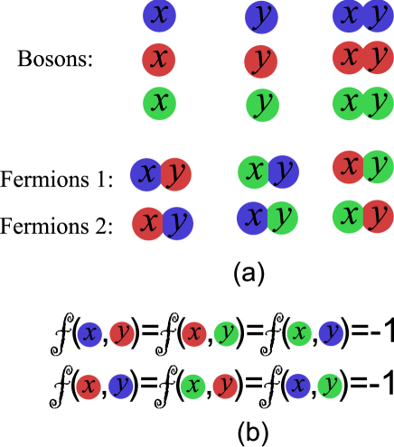
Figure 2: (a) Classification of excitations for the topological color code model (5), nine bosons and two families of fermions (b) The nontrivial phase arising from the braiding of different charges.

We describe all above excitations in terms of representation of the gauge group of the TCC. Before that, let us make a convention for colors which will be useful for subsequent discussions. We refer to colors by a bar operation $\bar{c}$ that transform colors cyclically as $\mathrm{\bar{r}=g}$, $\mathrm{\bar{g}=b}$ and $\mathrm{\bar{b}=r}$. The elements of the gauge group $\mathbf{Z_{2}}\times\mathbf{Z_{2}}$ are $\{\mathrm{e,r,b,g}\}$. Each excitation carries a topological charge. The corresponding topological charge can be labeled by the pair $(q,\chi)$, where $q\in\mathbf{Z_{2}}\times\mathbf{Z_{2}}$ and $\chi$ an irrep of this group AnyonicFermions . We label them as $\chi_{e}(c)=\chi_{c}(c)=-\chi_{c}(\bar{c})=1$. Therefore, there are nine bosons labeled by $(c,\chi_{e})$, $(e,\chi_{c})$ and $(c,\chi_{c})$ and six fermions $(c,\chi_{\bar{c}})$ and $(c,\chi_{\bar{\bar{c}}})$. Taking into account the vacuum with trivial charge $(e,\chi_{e})$, color code has sixteen topological charges or superselection sectors. Regarding the fusion process, fusion of two charges $(q,\chi_{c})$ and $(q^{\prime},\chi_{c^{\prime}})$ give rises to $(qq^{\prime},\chi_{c}\chi_{c^{\prime}})$ charge. Additionally, the braiding of charge $(q,\chi_{c})$ around charge $(q^{\prime},\chi_{c^{\prime}})$ produces the phase $\chi_{c}(q^{\prime})\chi_{c^{\prime}}(q)$. An excitation at a $c$-plaquette has $(c,\chi_{e})$ charge if $-B^{x}=B^{y}=1$, $(e,\chi_{c})$ charge if $B^{x}=-B^{y}=1$ and $(c,\chi_{c}$) charge if $B^{x}=B^{y}=-1$.

It is also possible to use both types of topological stabilizer codes, either toric codes or color codes, to go beyond homological operations. This corresponds to performing certain types of operations called code deformations, which may alter the topology of the surface allowing an extension of the computational capabilities of these 2D codes dennis_etal02 ; code_deformation07 ; rhg07 ; rh07 ; super09 .

Active error correction procedures are particularly interesting in the case of topological stabilizer codes. They give rise to connections with random statistical mechanical models like the random bond Ising model for the toric code dennis_etal02 and new random 3-body Ising models for color codes random_3Body . The whole phase diagram $p-T$ has been mapped out using Monte Carlo, which in particular gives the value of the error threshold $p_{c}$. This particular point can also be addressed using multicritical methodsohthreshold09 . There is experimental realization of topological error correction weibo_etal09 . Without external active error correction, the effect of thermal noise is the most challenging problem in toric codes AlickiFH-Kitaev1 ; AlickiFH-Kitaev2 ; AlickiHHH-Kitaev ; ipgap08b ; ipgap08a ; bravyi_terhal . Finite temperature effects of topological order in color codes has also been studied finite_temperatureTCC .

In all, the type of entanglement exhibited by topological color codes is very remarkable entanglementTCC ; ng_etal09 ; pakman_parnachev08 ; rico_briegel08 ; ecp09 ; dur_briegel07 ; vahid09 . A very illustrative way to see this is using the connection of the ground state of topological codes with standard statistical models by means of projective measurements ndb_07a ; br_07 ; ndb_07b ; stat_colorcodes ; ndrb08 ; hndb08 ; cdnb08 ; cdbm08 . For TCCs, this mapping yields the partition function of a 3-body classical Ising model on triangular lattices stat_colorcodes . This 3-body model is the same found in active error correcting techniques random_3Body , but without randomness since there is no noise produced by external errors. This type of statistical mapping allows us to test that different computational capabilities of color codes correspond to qualitatively different universality classes of their associated classical spin models. Furthermore, generalizing these statistical mechanical models for arbitrary inhomogeneous and complex couplings, it is possible to study a measurement-based quantum computation with a color code state and we find that their classical simulatability remains an open problem. This is in sharp contrast with toric codes which are classically simulable within this type of scheme br_07 .

II.2 The Model

In nature, we find that interactions are usually 2-body interactions. This is because interactions between particles are mediated by exchange bosons that carry the interactions (electromagnetic, phononic, etc.) between two particles.

The problem that arises is that for topological models, like the toric codes and color codes, their Hamiltonians have many-body terms (5). This could only achieved by finding some exotic quantum phase of nature, like FQHE, or by artificially enginering them somehow.

Here, we shall follow another route: try to find a 2-body Hamiltonian on a certain 2D lattice such that it exhibits the type of topological order found in toric codes and color codes. In this way, their physical implementation looks more accessible.

In fact, Kitaev honeycomb introduced a 2-body model in the honeycomb lattice that gives rise to an effective toric code model in one of its phases. It is a 2-body spin-$\frac{1}{2}$ model in a honeycomb lattice with one spin per vertex, and simulations based on optical lattices have been proposed duan03 .

The model features plaquette and strings constants of motion. Furthermore, it is exactly solvable, a property that is related to the 3-valency of the lattice where it is defined honeycomb ; Feng_et_al07 ; Yao_Kivelson07 ; baskaran_etal07 ; Yang_et_al07 ; si_yu08 ; mandal_surendran09 . It shows emerging free fermions in the honeycomb lattice. If a magnetic field is added, it contains a non-abelian topological phase (although not enough for universal quantum computation). Interestingly enough, another regime of the model gives rise to a 4-body model, which is precisely an effective toric code model. A natural question arises: Can we get something similar for color codes? We give a positive answer in what follows.

Motivated by these physical considerations related to a typical scenario in quantum many-body physics, either condensed matter, AMO physics or the like, we will seek a quantum spin Hamiltonian with the following properties:

i/ One of its phases must be the TCC.

ii/ To have two sets of plaquette operators generating a $\mathbf{Z}_{2}\times\mathbf{Z}_{2}$ local, i.e. gauge, symmetry.

iii/ To have string-nets and colored strings IOM as in the TCC, but in all coupling regimes.

Thus, the reasons behind demanding these properties are to guarantee that the sought after model will host the TCC. For instance, property i/ means that we must be able to generate the 2D color code Hamiltonian consistently at some lowest order in perturbation theory (PT). This we shall see in Sect.IV.2. Likewise, properties ii/ and iii/ are demanded in order to have the fundamental signatures regarding gauge symmetry and constants of motions associated with TCCs. Notice that we have not demanded that the model be exactly solvable. This is a mathematical requisite, rather than physical. We leave the door open for considering larger classes of models beyond exactly solvable models, which may be very interesting and contain new physics. For example, according to those properties, it would be possible to have models with a number of IOMs that scales linearly with $N$, the number of spins or qubits. Thus, the Kitaev model has a number of IOMs of $\frac{1}{2}N$.

Our purpose is to present first the 2-body quantum Hamiltonian in 2D AnyonicFermions , and then to analyze diverse possible mappings in later sections, like using bosonic and fermionic degrees of freedom. The analysis of the set of IOMs will play also a crucial role in the understanding of our model as we shall see in Sect.III

It is a 2-body spin-1/2 model in a ’ruby’ lattice as shown in Fig.3. We place one spin per vertex. Links come in 3 colors, each color representing a different interaction.

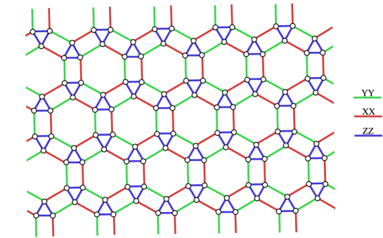
Figure 3: A lattice with coordination number 4 where the 2-body quantum lattice Hamiltonian for the color codes is defined according to spin-spin interactions coded by the colors of the links, as in (6). A plaquette can be distinguished by an inner hexagon, an outer hexagon and six blue triangles between them.

$$H=-\sum_{\langle i,j\rangle}J_{w}\sigma^{w}_{i}\sigma^{w}_{j},\ \ \ \ \ w=\begin{cases}x,&\text{ red links}\\ y,&\text{ green links}\\ z,&\text{ blue links}\end{cases}$$ (6)

For a suitable coupling regime, this model gives rise to an effective color code model. Furthermore, it exhibits new features, many of them not present in honeycomb-like models:

• Exact topological degeneracy in all coupling regimes ($4^{g}$ for genus $g$ surfaces).

• String-net integrals of motion.

• Emergence of 3 families of strongly interacting fermions with semionic mutual statistics.

• $\mathbf{Z}_{2}\times\mathbf{Z}_{2}$ gauge symmetry. Each family of fermions sees a different $\mathbf{Z}_{2}$ gauge subgroup.

III String Operators and Integrals of Motion

We can construct integrals of motion (IOM), $I\in\mathbf{P}_{n},[H_{\rm cc},I]=0$, following a pattern of rules assigned to the vertices of the lattice, as shown in Fig.4. These rules are constructed to attach a Pauli operator of type $\sigma^{x}_{i}$, $\sigma^{y}_{i}$ or $\sigma^{z}_{i}$ to each of the vertices $i$. The lines around the vertices, either wavy lines or direct lines, are pictured in order to join them along paths of vertices in the lattice that will ultimately translate into products of Pauli operators, which will become IOMs. Clearly, $\sigma^{z}_{i}$ operators are distinguished from the rest. The contribution of each qubit in the string operator is determined in terms of how it appears in the string. Its contribution may be determined by the outgoing red and green links which have the qubit as their end point in the string. In this case the $\sigma^{x}$ or $\sigma^{y}$ Pauli operators contribute in the string IOM . If a typical qubit crossed only by a wavy line as shown in Fig.4(a), it contributes a $\sigma^{z}$ Pauli operator in the string. To have a clear picture of string operators, a typical example has also been shown in Fig.4(b). Part of string is shown on the left and its expression will be the product of Pauli operators which have been inserted in open circles on the right. With such definitions for string operators and their supports on the lattice, now we turn on to analyze the relevance of strings to the model. In particular, we will construct elementary string operators with the local symmetry of the model. Therefore, in this way we are representing the local structure of the IOMs of our 2-body Hamiltonian (5). We will illustrate them with several examples of increasing complexity.

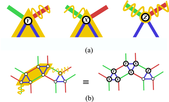
Figure 4: (a) A diagrammatic representation of the local structure of the integrals of motion of the 2-body Hamiltonian (6). The colored links represent different spin-spin interactions. (b) An example of contribution of Pauli operators in a string.

The ground state of a lattice model described by the Hamiltonian (5) is a superposition of all closed colored strings. Indeed, it is invariant under any deformations of colored strings as well as splitting of a colored string into other colors. In other words, the ground state is a string-net condensed state and supports topological order. The gauge group related to this topological order is $\mathbf{Z_{2}}\times\mathbf{Z_{2}}$. Such symmetry of topological color code can be realized via defining a set of closed string operators on the ruby lattice. We shall verify the gauge symmetry by identifying a set of string operators on the lattice of Fig.3.

Let us start by constructing the elementary string IOM as shown in Fig.5. They are denoted as $I=A,B,C$. They are closed since they have not endpoints left. The elementary closed strings are plaquettes. By a plaquette we mean an inner hexagon and an outer hexagon with six triangles in between. For a given plaquette it is possible to attach three string operators. For each closed string, the contribution of Pauli operators are determined based on outgoing red and green links or wavy lines as in Fig.4. Let $V_{f}$ stand for a set of qubits on a plaquette. Note that each plaquette contains $18$ qubits corresponding to six triangles around it. For first plaquette operator in Fig.5 we can write its explicit expression in terms of Pauli matrices as $S^{A}_{f}=\prod_{i\in V_{f}}\sigma^{\nu}_{i}$, where $f$ denotes the plaquette and $\nu=x,y$, depending on outgoing red or green links, respectively. Similarly the second plaquette operator has an expression as $S_{f}^{B}=\prod_{i\in V_{f}}\sigma^{\nu}_{i}$. The third string is only a closed wavy string which coincides to the inner hexagon of the plaquette. It’s expression is $S_{f}^{C}=\prod_{i\in V_{h}}\sigma^{z}_{i}$, where $V_{h}$ stands for six qubits on the inner hexagon. The three closed strings described above are not independent. Using the Pauli algebra, it is immediate to check that they satisfy $S^{C}_{f}=-S_{f}^{A}S_{f}^{B}$. Thus, there exist 2 independent IOMs per plaquette: this is the $\mathbf{Z}_{2}\times\mathbf{Z}_{2}$ local symmetry of the model Hamiltonian (6).

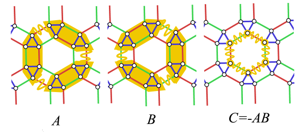
Figure 5: Schematic drawing of the plaquette IOMs according to the local rules in Fig.4. There are 3 IOMs denoted as $A,B,C$, but only 2 of them are independent. This corresponds to the symmetry $\mathbf{Z}_{2}\times\mathbf{Z}_{2}$ of the model.

Plaquette operators commute with each other and with any other IOM. If a IOM corresponds to a nontrivial cycle $c$, it is possible to find another IOM that anticommutes with it, namely one that corresponds to a cycle that crosses once $c^{\prime}$ . Thus, IOMs obtained from nontrivial cycles are not products of plaquette operators.

Each string operator squares identity since we are working with qubits. Plaquette operators corresponding to different plaquettes commute with each other and also with terms in Hamiltonian in (6) since they share in zero or even number of qubits. Therefore, the closed strings with the underlying symmetry obtained above define a set of integrals of motion. The number of integrals of motions is exponentially increasing. Let $3N$ be the total number of qubits, so the number of plaquettes will be $\frac{N}{2}$. Regarding to the gauge symmetry of the model, the number of independent plaquette operators is $N$. This implies that there are $2^{N}$ integrals of motion and allow us to divide the Hilbert space into $2^{N}$ sectors being eigenspaces of plaquette operators. However, for closed manifold, for example a torus, all plaquette operators can not be independently set to $+1$ or $-1$ because they are subject to some constraint. All other closed string operators that are homologous to zero, i.e. they are homotopic to the boundary of a plaquette, are just the product of these elementary plaquette operators. It is natural that all of them are topologically equivalent up to a deformation and commute with the Hamiltonian of the model.

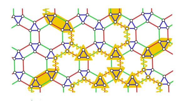
Figure 6: An example of a stringnet IOM. Notice the presence of branching points located around blue triangles of the lattice. This is a remarkable difference with respect to honeycomb models like the Kitaev model.

The most general configuration that we may have is shown in Fig.6. We call them string-nets IOM since in the context of our model, they can be thought of as the string-nets introduced to characterize topological orders levinwen05 . The key feature of these IOMs is the presence of branching points located at the blue triangles of the lattice. This is remarkable and it is absent in honeycomb 2-body models like the Kitaev model. When the string-nets IOM are defined on a simply connected piece of lattice they are products of plaquette operators. More generally, they can be topologically non-trivial and independent of plaquette operators.

As a special case of IOMs we have string configurations, i.e., paths without branching points. They correspond to the different homology classes of the manifold where the lattice is embedded , and are needed for characterization of the ground state manifold. Some examples are shown in Fig.7. They may be open or closed, depending on whether they have endpoints or not, respectively. Strings IOM are easier to analyze. String-nets IOM are products of strings IOM. For a given path, there exist 3 different strings IOM. These are denoted as $A,B,C$ in Fig.7.

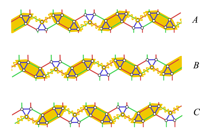
Figure 7: Examples of standard string configurations of IOMs, i.e., without branching points. For each path, we can in principle make 3 different assignments of IOMs, but again only 2 of them are independent as with plaquette IOMs. This is another manifestation of the $\mathbf{Z}_{2}\times\mathbf{Z}_{2}$ symmetry of the model.

We must introduce generators for the homology classes defining closed manifold. Homology classes of the torus are determined by realizing two nontrivial loops winding around the torus. In the Kitaev’s model there are only two independent such nontrivial closed loops. However, the specific construction of the lattice and contribution of the color make it possible to define for each homology class of the torus two independent nontrivial loops. These closed strings are no longer combination of plaquettes defined above. Let $S^{A}_{\mu}$ stand for such string, where $A$ and $\mu$ denote the type and homology class of the string. For each homology class of the manifold we can realize three different types of string operators depending on how the vertices of the lattice are crossed by the underlying string. Each qubit crossed by the string contributes a Pauli operator according to the rules in Fig.4. Again, using Pauli algebra we can see that only two of them are independent, as with the plaquette IOMs.

$$(-1)^{\frac{t}{2}}S^{A}_{\mu}S^{B}_{\mu}S^{C}_{\mu}=1,$$ (7)

where $t$ is the number of triangles on the string. To distinguish properly the three types we have to color the lattice. We could already use the colors to label strings. Strings are then red, green or blue. This is closely related to the topological color code topodistill ; AnyonicFermions . The latter relation shows that each string can be constructed of two other homologous ones, which is exactly the expression of the $\mathbf{Z_{2}}\times\mathbf{Z_{2}}$ gauge symmetry. Each non-contractible closed string operator of any homology commutes with all plaquette operators and with terms appearing in the Hamiltonian, so they are constant of motions. But, they don’t always commute with each other. In fact, if the strings cross once then

$$\left[S^{r}_{\mu},S^{r}_{\nu}\right]=0,$$ (8)

but

$$\left\{S^{r}_{\mu},S^{r^{\prime}}_{\nu}\right\}=0.$$ (9)

This latter anticommutation relation is a source of exact topological degeneracy Oshikawa_degeneracy of the model independent of phase we are analyzing it.

IV A Gapped Phase: The Topological Color Code

IV.1 Non-Perturbative Picture

In this subsection we discuss the ruby lattice is connected to the 2-colex even at the non-perturbative level. Then, in the subsequent sections we verify it using quantitative methods. From the previous discussion on IOMs, we have already seen a connection with the topological color codes. Now, we want to see how different strings introduced above are related to coloring of the lattice. To this end, consider the closed strings $A,B,C$ in Fig.5. The closed strings $A$ and $B$ can be visualized as a set of red and green links, respectively. With such visualization, we put forward the next step to color the inner hexagons of the ruby lattice: a colored link, say red, connect the red inner hexagons. Accordingly, other inner hexagons and links can be colored, and eventually we are left with a colored lattice. The emergence of the topological color code is beautifully pictured in Fig.8. Geometrically, it corresponds to shrinking the blue triangles of the original lattice into points, which will be referred as sites of a new emerging lattice, see Fig.8 (left). Thus, we realize that the inner hexagons and vertices of the model are colorable, see Fig.8 (middle): if we regard blue triangles as the sites of a new lattice, we get a honeycomb lattice, see Fig.8 (right). In fact, the model could be defined for any other 2-colex, not necessarily a hexagonal lattice.

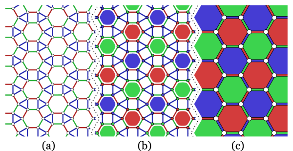
Figure 8: (color online) The three stages showing the emergence of the topological color code: (left) the original lattice for the 2-body Hamiltonian (6). The colors in the links denote the type of spin-spin interactions; (middle) a different coloring of the lattice is introduced based on the property that the hexagons are 3-colorable, as well as the vertices; (right) the hexagonal lattice obtained by shrinking to a point the blue triangles of the original lattice, which become sites in the final hexagonal lattice. This corresponds to the strong coupling limit in (15).

Connection to the 2-colexes can be further explored by seeing how strings on the ruby lattice correspond to the colored strings on the effective honeycomb lattice. To this end, consider a typical string-net on the ruby lattice as shown in Fig.9(a). This corresponds to a non-perturbative picture of the IOMs of the model. The fat parts of the string-net connect two inner hexagons with the same color. In this way, the corresponding string-net on the effective lattice can be colored as in Fig.9(b). The color of each part of the string-net on the effective honeycomb lattice is determined by seeing which colored inner hexagons on the ruby lattice it connects. Three colored strings cross each other at a branching point, and its expression in terms of Pauli matrices of sites are given by product of Pauli operators written adjacent to the sites. How they are determined, will be clear soon.

It is possible to use colors to label the closed strings on the honeycomb lattice. Before that, let us use a notation for Pauli operators acting on effective spins of honeycomb lattice $\tau^{\alpha}$, where $\alpha=x,y,z$. We indicate the labels $\alpha$ as $c|c:=z,\bar{c}|c:=x,\bar{\bar{c}}|c:=y$, where we are using a bar operator. To each c-plaquette, we attach three operators each of one color. Let $B^{c^{\prime}}_{f}$ denotes such operators, where low and up indices stand for c-plaquette $f$ and color of the closed string attached to the plaquette, respectively. With these notations, the plaquette operators read as follows:

$$B^{c^{\prime}}_{f}=\prod_{v\in f}\tau_{v}^{c^{\prime}|c},$$ (10)

where the product runs over all vertices of the c-plaquette $f$ in the honeycomb lattice in Fig.8(c). Thus, we can write the explicit expression of operators as follows:

$$B^{x}_{f}=B^{\bar{c}}_{f}=\prod_{v\in f}\tau_{v}^{\bar{c}|c}$$

$$B^{y}_{f}=B^{\bar{\bar{c}}}_{f}=\prod_{v\in f}\tau_{v}^{\bar{\bar{c}}|c}$$

$$B^{z}_{f}=-B^{c}_{f}=-\prod_{v\in f}\tau_{v}^{c|c}.$$ (11)

All these plaquette operators are constant of motions. Again, We can realize the gauge symmetry $\mathbf{Z_{2}}\times\mathbf{Z_{2}}$ through the relation $B^{x}_{f}B^{y}_{f}B^{z}_{f}=1$. On a compact manifold, for example on the torus, all plaquettes are not independent. They are subject to the following constraint:

$$\prod_{f\in\Lambda}B^{c}_{f}=(-1)^{N/2},$$ (12)

where the product runs over all plaquettes $f$ in the lattice $\Lambda$, and $N$ is the total number of plaquettes.

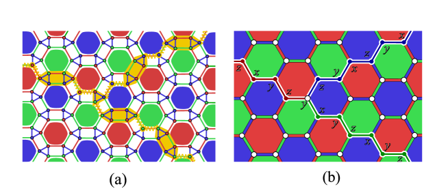
Figure 9: (color online) An illustraion of correspondence between (a) strings on the ruby lattice, corresponding to a non-perturbative picture, and (b)colored strings on the effective honeycomb lattice.

We can also realize noncontractible strings on the effective lattice which are rooted in the topological degeneracy of the model. They are just the IOMs in Fig.7 when reduced on the effective honeycomb lattice. Once the inner hexagons of ruby lattice are colored, they correspond to colored strings as in Fig.9. Let $S^{c}_{\mu}$ stands for such string, where indices $\mu$ and $c$ denote the homology and color of the string, respectively. This string operator is tensor product of Pauli operators of qubits lying on the string. Namely, the string operator is

$$S^{c}_{\mu}=\prod_{v}\tau^{c^{\prime}|c}_{v}.$$ (13)

The contribution of each qubit is determined by the color of the hexagon that the string turns on it, see Fig.10. For example in the string $S_{1}$ shown in Fig.10, the color of the plaquettes appearing in (13) marked by light circles. With this definition for string operators, the contribution of Pauli operators in the string-net on the effective lattice in Fig.9(b) are reasonable. Non-contractible colored strings are closely related to the topological degeneracy of the model, since they commute with color code Hamiltonian(5) being integrals of motion, but not always with each other. In fact, two strings differing in both homology and color anticommute, otherwise they commute. For example let us consider two non-contractible closed strings $S_{1}$ and $S_{2}$ corresponding to different homologies of the torus. As shown in Fig.10, they share two qubits. First, suppose both strings are of blue type. The contribution of Pauli operators of these two qubits in string $S_{1}$ is $\tau^{y}_{1}\tau^{x}_{2}$, while for string $S_{2}$ the contribution is $\tau^{x}_{1}\tau^{y}_{2}$ implying $[S^{b}_{1},S^{b}_{2}]=0$. Then, let $S_{2}$ be a green string. In this case the contribution of qubits will be $\tau^{y}_{1}\tau^{z}_{2}$, which explicitly shows that $\{S^{b}_{1},S^{g}_{2}\}=0$. The interplay in (7) can be translated into an interplay between color and homology as follows.

$$(-1)^{\frac{s}{2}}S^{c}_{\mu}S^{\bar{c}}_{\mu}S^{\bar{\bar{c}}}_{\mu}=1,$$ (14)

where $s$ is the number of sites on the string. This interplay makes the ground state subspace of the color code model be a string-net condensed phase.

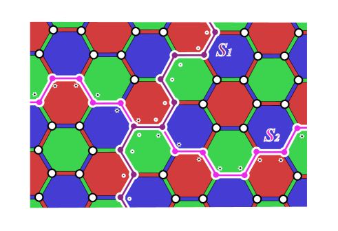
Figure 10: (color online) A piece of effective lattice. The strings $S_{1}$ and $S_{2}$ correspond to different homology classes of the manifold. Their expression in terms of Pauli operators are given by their associated color and the fact that how they turn on plaquettes on the lattice.

IV.2 Degenerate Perturbation Theory: Green Function Formalism

In this subsection we put the above correspondence between original 2-body lattice Hamiltonian and color code model on a quantitative level. In fact, there is a regime of coupling constants in which one of the phases of the 2-body Hamiltonian reproduces the TCC many-body structure and physics. In particular, we show that this corresponds to the following set of couplings in the original 2-body Hamiltonian

$$J_{x},J_{y},J_{z}>0,~{}~{}~{}J_{x},J_{y}\ll J_{z},$$ (15)

that is, a strong coupling limit in $J_{z}$. The topological color code effectively emerges in this coupling regime. This can be seen using degenerate perturbation theory in the Green function formalism. Let $H=H_{0}+V$ be a Hamiltonian describing a physical system with two-body interaction, and we regard the $\|V\|$, the norm of $V$, be very small in comparison with the spectral gap of unperturbed $H_{0}$. We also suppose that $H_{0}$ has a degenerate ground-subspace which is separated from the excited states by a gap $\Delta$. The effect of $V$ will be to break the ground state degeneracy in some order of perturbation. Now the interesting question is whether it is possible to construct an effective Hamiltonian, $H_{\mathrm{eff}}$, which describes the low energy properties of the perturbed Hamiltonian $H$. The effective Hamiltonian arises at orders of perturbation that break the ground state degeneracy. From the quantum information perspective the Hamiltonian $H$ acts on the physical qubits while the effective Hamiltonian acts on the logical qubits projected down from the physical qubits.

We will clarify that how many-body Hamiltonian in (5) will present an effective description of low lying states of the 2-body Hamiltonian (6). We use the perturbation about the Hamiltonian in (6) considering the coupling regim (15). Here, the qubits on the triangles are physical qubits, and logical qubits are those living at the vertices of the 2-colex. We refer to triangles as sites, since they correspond to the vertices of the 2-colex. Thus a triangle will be shown by index $v$ and its vertices by Latin indices $i,j$. In fact the low lying spectrum of 2-body Hamiltonian encodes the following projection from the physical qubits to the logical ones at each site:

$$P_{v}=|\!\Uparrow\rangle\langle\uparrow\uparrow\uparrow\!|+|\!\Downarrow\rangle\langle\downarrow\downarrow\downarrow\!|,$$ (16)

where $|\!\Uparrow\rangle$ and $|\!\Downarrow\rangle$ stands for the two states of the logical qubit at site $v$, and $|\!\uparrow\rangle$ ($|\!\downarrow\rangle$) is usual up (down) states of a single spin in computational bases.

To this end, we split the 2-body Hamiltonian into two parts. The unperturbed part is $H_{0}=-J_{z}\sum_{\mathrm{b}-link}\sigma^{z}_{i}\sigma^{z}_{j}$. In the limit of strong Ising interaction the system is polarized. The interactions between neighboring qubits on different triangles are included in $V$. They are $\sigma^{x}_{i}\sigma^{x}_{j}$ and $\sigma^{y}_{i}\sigma^{y}_{j}$ corresponding to red and green links in Fig.3, respectively. So, the transverse part of the Hamiltonian is

$$V=-J_{x}\sum_{\mathrm{r}-link}\sigma^{x}_{i}\sigma^{x}_{j}-J_{y}\sum_{\mathrm{g}-link}\sigma^{y}_{i}\sigma^{y}_{j}.$$ (17)

In the case when $J_{z}\gg J_{x},J_{y}$ the low lying excitations above the fully polarized state can be treated perturbatively.

The unperturbed part of the Hamiltonian, $H_{0}$, has a highly degenerate ground space because, for each triangle, two fully polarized states $|\!\uparrow\uparrow\uparrow\rangle$ and $|\!\downarrow\downarrow\downarrow\rangle$ have same energy. The ground state subspace is spanned by all configurations of such polarized states. Let $N$ be the number of triangles of the lattice. The ground state energy is $E_{0}^{(0)}=-3NJ_{z}$ and the dimension of the ground space of the $H_{0}$ or ground state degeneracy reads $g_{0}=2^{N}$. The first excited state is produced by exciting one of triangles and has energy $E_{1}^{(0)}=(-3N+4)J_{z}$ with degeneracy $g_{1}=6N2^{N-1}$. The second excited state has energy $E_{1}^{(0)}=(-3N+8)J_{z}$ with degeneracy $g_{2}=18N(N-1)2^{N-2}$, and so on and so forth.

We analyze the effect of $V$ on the ground state manifold by using the degenerate perturbation theoryBergman_dpt in couplings $J_{x}$ and $J_{y}$. We are interested in how ground state degeneracy is lifted by including the interaction between triangles perturbatively. Let $\mathcal{L}$ stand for the ground state manifold with energy $E^{(0)}_{0}$ and let $P$ be the projection onto the ground state manifold $\mathcal{L}$. The projection is obtained from the degenerate ground states as follows:

$$P=\prod_{v\in\Lambda}P_{v}~{}~{}~{}~{}~{}~{}~{}~{},~{}~{}~{}~{}~{}~{}P_{v}=|\!\Uparrow\rangle\langle\uparrow\uparrow\uparrow\!|+|\!\Downarrow\rangle\langle\downarrow\downarrow\downarrow\!|.$$ (18)

Using the projection and Green’s function we can calculate the effective Hamiltonian at any order of Perturbation theory. The eigenvalues of the effective Hamiltonian $H_{\mathrm{eff}}$ appear as the poles of the Green function $G(E)=P[1/(E-H)]P$. The effect of perturbation can be recast into the self-energy $\Sigma(E)$ by expressing the Green’s function as $1/(E-E^{(0)}_{0}-\Sigma(E))$. So, the effective Hamiltonian will be

$$H_{\mathrm{eff}}=\sum^{\infty}_{l=0}H^{(l)}_{\mathrm{eff}}=E^{(0)}_{0}+\Sigma(E).$$ (19)

The self-energy can be represented in terms of Feynman diagrams and can be computed for any order of perturbation:

$$\Sigma(E)=PV\sum^{\infty}_{n=0}\mathcal{U}^{n}P,$$ (20)

where $\mathcal{U}=[1/(E-H_{0})](1-P)V$. The energy $E$ can also be expanded at different orders of perturbation, $E=E^{(0)}_{0}+\sum^{\infty}_{l=1}E^{(l)}_{0}$. Now, we are at the position to determine different orders of perturbation. Each term of $V$ acts on two neighboring physical qubits of different triangles. At a given order of perturbation theory, there are terms which are product of $\sigma^{x}$ and $\sigma^{y}$ acting on the ground state subspace. Each term when acts on the ground state manifold brings the ground state into an excited state. However, there may be a specific product of the $\sigma^{x}$ and $\sigma^{y}$ which takes the ground state into itself, i.e. preserve the polarized configurations of triangles.

At zeroth-order the effective Hamiltonian will be trivial $H^{(0)}_{\mathrm{eff}}=E^{(0)}_{0}$. The first-order correction is given by the operator

$$H^{(1)}_{\mathrm{eff}}=PVP.$$ (21)

The effect of $V$ is to move the states out of the ground state manifold because each term either $\sigma^{x}\sigma^{x}$ or $\sigma^{y}\sigma^{y}$ flip two qubits giving rise to two triangles being excited, i.e $VP=P_{2}VP$, where the operator $P_{2}$ is the projection to second excited state manifold. Therefore, $PVP=0$, and there is no first-order correction to the ground state energy.

The second-order correction to the ground state will be the eigenvalues of the following operator.

$$H^{(2)}_{\mathrm{eff}}=PVG^{\prime}(E^{(0)}_{0})VP+PVP,$$ (22)

where the operator $G^{\prime}(E)=1/(E-H_{0})$ is the unperturbed Green’s function and the superscript prime stands for the fact that its value be zero when acts on the ground state. The second-order correction only shifts the ground state energy, and therefore, the second-order effective Hamiltonian acts trivially on ground state manifold,

$$H^{(2)}_{\mathrm{eff}}=3N\frac{J^{2}_{x}+J^{2}_{y}}{-8J_{z}}P.$$ (23)

In fact the first $V$ flips the qubits and the second $V$ flips them back. As we go to higher order of perturbation theory the terms become more and more complicated. However, if the first-order is zero as in our case, the terms becomes simpler. Thus, the third-order of perturbation will be zero and will leave corrections to energy and ground state intact:

$$H^{(3)}_{\mathrm{eff}}=PV\left(G^{\prime}(E^{(0)}_{0})V\right)^{2}P=0.$$ (24)

The forth-order of perturbation theory contributes the following expression to the correction of ground state manifold:

$$H^{(4)}_{\mathrm{eff}}=PV\left(G^{\prime}(E^{(0)}_{0})V\right)^{3}P-E^{(2)}_{0}PV\left(G^{\prime}(E^{(0)}_{0})\right)^{2}VP,$$

(25)

where $E^{(2)}_{0}$ is the second order correction to the ground state energy obtained in (23). The first term includes four $V$ and must act in the ground state in which the last $V$ returns the state to the ground state manifold. The second term is like the second-order. There are many terms which must be calculated. However, since the forth-order only gives a shift to the ground state energy, we don’t need them explicitly. So, we can skip the forth-order. Fifth-order correction yields terms each containing odd number of $V$, so it gives zero contribution to the effective Hamiltonian.

The sixth-order of perturbation leads to the following long expression.

$$H^{(6)}_{\mathrm{eff}} = PV\left(G^{\prime}(E^{(0)}_{0})V\right)^{5}P-E^{(4)}_{0}PV\left(G^{\prime}(E^{(0)}_{0})\right)^{2}VP$$ (26)

$$+\left(E^{(2)}_{0}\right)^{2}PV\left(G^{\prime}(E^{(0)}_{0})\right)^{3}VP$$

$$-E_{0}^{(2)}PV\left(G^{\prime}(E^{(0)}_{0})\right)^{2}V\left(G^{\prime}(E^{(0)}_{0})V\right)^{2}P$$

$$-E_{0}^{(2)}PVG^{\prime}(E^{(0)}_{0})V\left(G^{\prime}(E^{(0)}_{0})\right)^{2}VG^{\prime}(E^{(0)}_{0})VP$$

$$-E_{0}^{(2)}PV\left(G^{\prime}(E^{(0)}_{0})V\right)^{2}\left(G^{\prime}(E^{(0)}_{0})\right)^{2}VP.$$

Apart from the first term, other terms contain two or four $V$ and as we discussed in the preceding paragraphs they only contribute a shift in the ground state energy. However, the first term gives the first non-trivial term breaking in part the ground state degeneracy. In the sixth order correction, there are some terms which are the product of $\sigma^{x}\sigma^{x}$ and $\sigma^{y}\sigma^{y}$ associated to the red and green links of the ruby lattice. Some particular terms, as seen below, may map ground state subspace into itself. For instance, consider the following product of links around an inner hexagon

$$\prod_{<i,j>}\sigma^{w}_{i}\sigma^{w}_{j}=\pm\prod_{i\in V_{h}}\sigma_{i}^{z},$$ (27)

where the first product runs over three red and three green links making an inner hexagon, $V_{h}$ stands for the set of its vertices and the prefactor $\pm$ depends on the ordering of links in the product. The action of a $\sigma^{z}$ on one vertex (qubit) of a triangle encodes an logical $\tau_{v}^{z}$ operator acting on the associated vertex of lattice $\Lambda$. This can explicitly be seen from the following relation:

$$\tau_{v}^{z}=P_{v}\sigma^{z}P_{v}=|\!\Uparrow\rangle\langle\Uparrow\!|-|\!\Downarrow\rangle\langle\Downarrow\!|,$$ (28)

where $\sigma^{z}$ acts on one of the vertices of a triangle and $P_{v}$ is the projection defined in (16). Thus, the expression of (27) can be related to the plaquette operator $B^{z}_{f}=-\prod\tau_{v}^{z}$, where the index $f$ denotes a plaquette of effective lattice $\Lambda$ as in Fig.1 and product runs over six sites around it. Now we go on to pick up the sixth-order correction to the ground state manifold. There are many terms which must be summed. Sixth-order correction up to a numerical constant contributes the following expression to the effective Hamiltonian:

$$H^{(6)}_{\mathrm{eff}}=\mathrm{constant}-\delta\frac{J_{x}^{3}J_{y}^{3}}{J_{z}^{5}}\sum_{f}B^{z}_{f},$$ (29)

where $\delta$ is a positive numerical constant arising from summing up $720$ terms related to the order of product of six links around an inner hexagon of ruby lattice. Although, its exact numerical value is not important, but knowing its sign is essential for our subsequent discussions. As it is clear from the first term in (26), five Green’s functions and six $V$ in the perturbation contribute a minus sign to the expression. This minus sign together with the sign appearing in (27) enforce the coefficient $\delta$ be a positive constant. Now it is simple to realize how the vectors in the ground state manifold rearranged. Trivially, all plaquette operators $B^{z}_{f}$ commute with each other and their eigenvalues are $\pm 1$. All polarized vectors in $\mathcal{L}$ are the eigenvector of the effective Hamiltonian emerging at sixth-order. But, those are ground states of the effective Hamiltonian in (29) which are eigenvectors of all plaquette operators $B^{z}_{f}$ with eigenvalue $+1$. Thus, highly degenerate ground state of the unperturbed Hamiltonian is broken in part. The same plaquette operators $B^{z}_{f}$ also appear at higher order of perturbation. For example, at eighth-order. Instead of giving the rather lengthy expression of the eighth-order correction, we only keep terms resulting in the plaquette operators as follows:

$$H^{(8)}_{\mathrm{eff}}=\mathrm{constant}-\beta\frac{J_{x}^{5}J_{y}^{3}+J_{x}^{3}J_{y}^{5}}{J_{z}^{7}}\sum_{f}B^{z}_{f},$$ (30)

where $\beta>0$. This term is added to the one in (29) to give the effective Hamiltonian up to eighth-order, but the ground state structure remains unchanged. Further splitting in the ground state manifold is achieved by taking into account the ninth-order of perturbation. The expression of ninth-order is very lengthy. However, the first term of the expression containing nine $V$ gives some terms being able of mapping the ground state manifold into itself in a nontrivial way. These terms map a polarized triangle, say up, to a down one. Indeed, when one or two qubits of the polarized triangle gets flipped, its state is excited. However, flipping three qubits of the triangle returns back the ground state onto itself. This process encodes $\tau^{x}$ and $\tau^{y}$ logical operators acting on logical qubits arising through the projection. Let $\sigma^{x}_{1}$, $\sigma^{x}_{2}$ and $\sigma^{y}_{3}$ act on three qubits of a triangle. The encoded $\tau^{y}$ operator will be

$$\tau_{v}^{y}=P_{v}\sigma^{x}_{1}\sigma^{x}_{2}\sigma^{y}_{3}P_{v}=-i|\!\Uparrow\rangle\langle\Downarrow\!|+i|\!\Downarrow\rangle\langle\Uparrow\!|.$$ (31)

If $\sigma^{x}_{1}$, $\sigma^{y}_{2}$ and $\sigma^{y}_{3}$ act on three qubits of a triangle, the encoded $\tau^{x}$ logical operator will be

$$-\tau_{v}^{x}=P_{v}\sigma^{x}_{1}\sigma^{y}_{2}\sigma^{y}_{3}P_{v}=-|\!\Uparrow\rangle\langle\Downarrow\!|-|\!\Downarrow\rangle\langle\Uparrow\!|.$$ (32)

As we already pointed out a plaquette of the ruby lattice is made up of an inner hexagon, an outer hexagon and the six blue triangles. It is possible to act on the polarized space of the blue triangles by making two different combinations of $9$ link interactions: i/ Applying $6$ link interactions on the outer hexagon (three of them of XX type and another three of YY type), times 3 link interactions of red type on the inner hexagon. Notice that every vertex of the blue triangles in the plaquette gets acted upon these $9$ link interactions. The resulting effective operator is of type $\tau^{y}$ due to (31). ii/ Applying $6$ link interactions on the outer hexagon, times $3$ link interactions of green type. Then, the resulting effective operator is of type $\tau^{x}$ due to (32).

The effective Hamiltonian at this order then reads

$$H^{(9)}_{\mathrm{eff}} = PV\left(G^{\prime}(E^{(0)}_{0})V\right)^{8}P+...$$

$$= \mathrm{constant}-\gamma\frac{J_{x}^{6}J_{y}^{3}}{J_{z}^{8}}\sum_{f}B^{y}_{f}-\gamma\frac{J_{x}^{3}J_{y}^{6}}{J_{z}^{8}}\sum_{f}B^{x}_{f}.$$

Again, the sign of coefficient $\gamma$ is important. Nine $V$’s, six $\tau^{x}$ or $\tau^{y}$, and eight Green’s function imply that the $\gamma$ must have positive sign.

Putting together all above obtained corrections lead to an effective Hamiltonian encoding color code as its ground statetopodistill ; entanglementTCC . Therefore, up to constant terms, the effective Hamiltonian reads as follows

$$H_{\mathrm{eff}}=-k_{z}\sum_{f}B^{z}_{f}-k_{x}\sum_{f}B^{x}_{f}-k_{y}\sum_{f}B^{y}_{f},$$ (34)

where the $k_{z}$, $k_{x}$ and $k_{y}$ are positive coefficients arising at different orders. Since $B^{x}_{f}B^{y}_{f}=B^{z}_{f}$, the above effective Hamiltonian is just the many-body Hamiltonian of the color code as in (1). The terms appearing in the Hamiltonian mutually commute, so the ground state will be the common eigenvector of plaquette operators. Since each plaquette operator squares identity, the ground state subspace, $\mathcal{C}$, spanned by vectors which are common eigenvectors of all plaquette operators with eigenvalue $+1$, i.e

$$\mathcal{C}=\{|\psi\rangle:~{}B^{x}_{f}|\psi\rangle=|\psi\rangle,~{}B^{y}_{f}|\psi\rangle=|\psi\rangle~{};~{}~{}\forall f\}.$$ (35)

The group of commuting boundary closed string operators can be used as an alternative way to find the terms appearing in the effective HamiltonianKells . As we pointed out in the preceding section, the non-zero contribution from various orders of perturbation theory results from the product of red and green links which preserve the configurations of the polarized triangles, i.e maps ground state manifold onto itself. For instance consider the elementary plaquette operator $A$ corresponding to a closed string in Fig.5. Each triangle contributes $\sigma^{y}\sigma^{y}\sigma^{x}$ to the expression of operator which is projected to $\tau^{x}$ as in (32). Thus, the effective representation of plaquette operator reads as follows:

$$PS_{f}^{A}P\rightarrow B^{x}_{f}.$$ (36)

Plaquette operators $S_{f}^{B}$ and $S_{f}^{C}$ can also be recast into the effective forms as follows:

$$PS_{f}^{B}P\rightarrow B^{y}_{f}~{},~{}~{}~{}~{}~{}~{}~{}~{}~{}~{}~{}PS_{f}^{C}P\rightarrow-B^{z}_{f}.$$ (37)

These are lowest order contributions to the effective Hamiltonian as we obtained in (34). Higher order of perturbation will be just the product of effective plaquette operators. The nontrivial strings winding around the torus will have also effective representations and appear at higher orders of perturbation. In general, every string-net IOM on the ruby lattice are projected on an effective one as in Fig.9.

V Bosonic Mapping

As we stated in Sect.III, one of the defining properties of our model is the existence of non-trivial integrals of motion IOM, called string-nets. As a particular example, the Kitaev’s model on the honeycomb lattice has strings IOMs, but not string-nets. We are interested in models in which the number of IOMs is proportional to the number of qubits in the lattice, i.e.,

$$I=\eta N_{q},$$ (38)

where $I$ is the number of IOMs, $N_{q}$ is the number of qubits (spins) in the lattice, and $\eta$ is a fraction: $\eta=\frac{1}{2}$ for the Kitaev model honeycomb , $\eta=\frac{1}{3}$ for our model in (6) AnyonicFermions . The fact that $\eta$ is a fraction $\eta\leq 1$ implies that these models based on string-net IOMs will not necessarily be exactly solvable. In the Kitaev’s model, it turns out to be exactly solvable using an additional mapping with Majorana fermions, but this need not be a generic case. Therefore, we need to resort to other techniques in order to study the physical properties of these models. We consider here and next section, approximate methods based on bosonic and fermionic mappings. The application of the bosonic method to our model is based on a mapping from the original spins on the blue triangles to hardcore bosons with spin AnyonicFermions . With this mapping, it is possible to use the PCUTs approach (Perturbative Continuous Unitary Transformations) pcut_Uhrig . This is inspired by the RG method based on unitary transformation introduced by Wegner (the Similarity RG method) pcut_Wegner . Originally, the PCUTs method was applied to the Kitaev model boson_honeycomb . As we will see below, the method paves the way to go beyond the perturbation approach presented in the preceding section which fits into a sector without any hard-core boson. The physics at other sectors is very promising and we study it here. Emergence of three families of strongly interacting anyonic fermions and invisible charges are among them, which are not present in the Kitaev’s model or its variants. To start with, let us set for simplicity $J_{z}=1/4$, and consider the extreme case of $J_{x}=J_{y}=0$. In this case the system consists of isolated triangles. The ground states of an isolated triangle are polarized states $|\!\uparrow\uparrow\uparrow\rangle$ and $|\!\downarrow\downarrow\downarrow\rangle$ with energy $-3/4$. The excited states that appear by flipping spins are degenerate with energy $1/4$. In this limit, the spectrum of whole system is made of equidistance levels being well-suited for perturbative analysis of the spectrum: Green’s function formalism as discussed in the preceding section, which may capture only the lowest orders of perturbation or another alternative approach based on the PCUT. The change from the ground state to an exited state can be interpreted as a creation of particles with energy $+1$. This suggest an exact mapping from the original spin degrees of freedom to quasiparticles attached to effective spins. The mapping is exact, i.e. we don’t miss any degrees of freedom. Such a particle is a hard-core boson. At each site, we attach such a boson and also an effective spin-$\frac{1}{2}$. Let choose the following bases for the new degrees of freedom

$$|a,d\rangle=|a\rangle\otimes|d\rangle,~{}~{}~{}~{}~{}~{}a=\Uparrow,\Downarrow,~{}~{}~{}~{}d=0,\mathrm{r,g,b},$$ (39)

where $a$ and $d$ stand for states of the effective spin and quasiparticle attached to it. The Hilbert space $\mathcal{H}_{C}$ representing the hard-core bosons is four dimensional spanned by bases $\{|0\rangle,|\mathrm{r}\rangle,|\mathrm{g}\rangle,|\mathrm{b}\rangle\}$. Now the following construction relates the original spin degrees of freedom and new ones in (39)

$$|\!\Uparrow,0\rangle\equiv|\!\uparrow\uparrow\uparrow\rangle,~{}~{}~{}~{}~{} |\!\Downarrow,0\rangle\equiv|\!\downarrow\downarrow\downarrow\rangle$$

$$|\!\Uparrow,\mathrm{r}\rangle\equiv|\!\uparrow\downarrow\downarrow\rangle,~{}~{}~{}~{}~{} |\!\Downarrow,\mathrm{r}\rangle\equiv|\!\downarrow\uparrow\uparrow\rangle$$

$$|\!\Uparrow,\mathrm{g}\rangle\equiv|\!\downarrow\uparrow\downarrow\rangle,~{}~{}~{}~{}~{} |\!\Downarrow,\mathrm{g}\rangle\equiv|\!\uparrow\downarrow\uparrow\rangle$$

$$|\!\Uparrow,\mathrm{b}\rangle\equiv|\!\downarrow\downarrow\uparrow\rangle,~{}~{}~{}~{}~{} |\!\Downarrow,\mathrm{b}\rangle\equiv|\!\uparrow\uparrow\downarrow\rangle.$$ (40)

Within such mapping, the effective spins and hard-core bosons live at the sites of the effective hexagonal lattice $\Lambda$ in Fig. 8(c). Recall that this lattice is produced by shrinking the triangles. At each site we can introduce the color annihilation operator as $b_{c}:=|0\rangle\langle c|$. The number operator $n$ and color number operator $n_{c}$ are

$$n:=\sum_{c}n_{c},\qquad n_{c}:=b^{\dagger}_{c}b_{c}.$$ (41)

Annihilation and creation operators anticommute on a single site, and commute at different sites, that is why they are hard-core bosons. We can also label the Pauli operators of original spins regarding to the their color in Fig. 8(b) as $\sigma^{w}_{c}$ with $c=\mathrm{r,g,b}$. The mapping in (40) can be expressed in operator form as follows

$$\sigma^{z}_{c}\equiv\tau^{z}\otimes p_{c},\quad\sigma^{\nu}_{c}\equiv\tau^{\nu}\otimes(b_{c}^{\dagger}+b_{c}+s_{\nu}r_{c}),$$ (42)

where $\nu=x,y$, $s_{x}:=-s_{y}:=1$, the symbols $\tau$ denote the Pauli operators on the effective spin and we are using the color parity operators $p_{c}$ and the color switching operators $r_{c}$ defined as

$$p_{c}:=1-2(n_{\bar{c}}+n_{\bar{\bar{c}}}),\qquad r_{c}:=b^{\dagger}_{\bar{c}}b_{\bar{\bar{c}}}+b^{\dagger}_{\bar{\bar{c}}}b_{\bar{c}}.$$ (43)

Now we can forget the original ruby lattice and work on the effective lattice in which the bosons are living at its sites. With the above identification for Pauli operators, the 2-body Hamiltonian in (6) can be written in this language. Before that, let fix a simplified notation. All spin and bosonic operators act on the sites of the effective lattice. We refer to a site by considering its position relative to a reference site: the notation $O_{,c}$ means $O$ applied at the site that is connected to a site of reference by a $c$-link. The 2-body Hamiltonian then becomes

$$H=-3N/4+Q-\sum_{\Lambda}\sum_{c\neq c^{\prime}}J_{c^{\prime}|c}\,T_{c}^{c^{\prime}},$$ (44)

with $N$ the number of sites, $Q:=\sum_{\Lambda}n$ the total number of hardcore bosons, the first sum running over the $N$ sites of the reduced lattice, the second sum running over the 6 combinations of different colors $c,c^{\prime}$ and

$$T_{c}^{c^{\prime}}=u_{c}^{c^{\prime}}+\frac{t_{c}^{c^{\prime}}+v_{c}^{c^{\prime}}}{2}+\frac{r_{c}^{c^{\prime}}}{4}+\mathrm{h.c.},$$ (45)

a sum of several terms for an implicit reference site, according to the notation convention we are using. The meaning of the different terms in (45) is the following. The operator $t_{c}^{c^{\prime}}$ is a $c$-boson hopping, $r_{c}^{c^{\prime}}$ switches the color of two ${\bar{c}}$- or ${\bar{\bar{c}}}$-bosons, $u_{c}^{c^{\prime}}$ fuses a $c$-boson with a ${\bar{c}}$-boson (or a ${\bar{\bar{c}}}$-boson) to give a ${\bar{\bar{c}}}$-boson (${\bar{c}}$-boson) and $v_{c}^{c^{\prime}}$ destroys a pair of $c$-bosons. The explicit expressions are

$$t_{c}^{c^{\prime}}:=\tau_{c}^{c^{\prime}}b_{c}b^{\dagger}_{c,c^{\prime}},\qquad r_{c}^{c^{\prime}}:=\tau_{c}^{c^{\prime}}r_{c}r_{c,c^{\prime}},$$

$$u_{c}^{c^{\prime}}:=s_{c^{\prime}|c}\tau_{c}^{c^{\prime}}b_{c}r_{c,c^{\prime}},\qquad v_{c}^{c^{\prime}}:=\tau_{c}^{c^{\prime}}b_{c}b_{c,c^{\prime}},$$ (46)

where we are using the notation

$$\tau_{c}^{c^{\prime}}:=\tau^{c^{\prime}|c}\tau_{,c^{\prime}}^{c^{\prime}|c}.$$ (47)

We can also describe the plaquette IOM operators in Fig. 5 in terms of spin-boson degrees of freedom by means of the mapping in (42). For each plaquette $f$ and color $c$, the plaquette operator is expressed as

$$S_{f}^{c}:=\prod_{v\in f}\tau_{v}^{c|c^{\prime}}p_{c^{\prime}\star c},$$ (48)

where $c^{\prime}$ is the color of the plaquette $f$, the product runs through its sites and $\star$ is just a convenient symmetric color operator defined by

$$c\star c:=c,\qquad c\star{\bar{c}}:={\bar{c}}\star c:={\bar{\bar{c}}}.$$ (49)

The relation in (48) is just a generalization of plaquette operators in (11) to other sectors of the system. In fact taking the zero particle sector, the expressions in (11) are recovered. In the same way the nontrivial string operators in Fig.7 can be described with the above mapping as

$$S^{c}_{\mu}:=\prod_{v\in\mu}\tau_{v}^{c|c^{\prime}}p_{c\star c^{\prime}},$$ (50)

where $\mu$ denotes the homology class of the string. On closed surfaces, not all plaquette operators are independent. They are subject to the following constraints

$$\prod_{f\in\Lambda}S_{f}^{c}=(-1)^{N/2},\qquad\prod_{c=\mathbf{r,g,b}}S_{f}^{c}=(-1)^{s/2},$$ (51)

where $s$ is the number of sites of a given plaquette $f$. The first equation can be further divided into products over subsets of plaquettes giving rise to other constants of motion, the so called color charges, as

$$\prod_{f\in\Lambda_{{\bar{c}}}}S_{f}^{\bar{c}}\prod_{f\in\Lambda_{{\bar{\bar{c}}}}}S_{f}^{\bar{\bar{c}}}=\prod_{f\in\Lambda_{{\bar{\bar{c}}}}}S_{f}^{c}\prod_{f\in\Lambda_{c}}S_{f}^{\bar{c}}=\prod_{\Lambda}p_{c}.$$ (52)

In these products the spin degrees of freedom are washed out, since they appear twice and consequently square identity. By use of equation (43), the product over parity operators can be written as

$$\chi_{\Lambda}(c)=\prod_{\Lambda}p_{c}=(-1)^{Q_{{\bar{c}}}+Q_{{\bar{\bar{c}}}}},$$ (53)

where $Q_{c}=\sum_{\Lambda}n_{c}$ is the total number of $c$-bosons. It is simple to check that the above equation commutes with Hamiltonian in (44). For each family of bosons we can attach a charge. We suppose that each $c$-boson carries a charge as $\chi_{\mathrm{c}}$, that is, an irrep of the gauge group. In particular, the Hamiltonian preserves the following total charge

$$\chi_{\Lambda}:=\chi_{\mathrm{r}}^{Q_{\mathrm{r}}}\chi_{\mathrm{g}}^{Q_{\mathrm{g}}}\chi_{\mathrm{b}}^{Q_{\mathrm{b}}}.$$ (54)

V.1 Emerging particles: anyonic fermions

Equation (52) could already suggest that the parity of vortices are correlated to the parity of the number of bosons. In particular, creation of a $c$-boson changes the vorticity content of the model.

The statistics of vortices depend on their color and type as in Fig.2. But what about the statistics of $c$-bosons? As studied in wen_statistics , the statistics of quasiparticles can be examined using the hopping terms. These hopping terms are combined so that two quasiparticles are exchanged. In addition to usual hopping terms, we also need for composite hopping , that is, a $c$-boson hops from a $c$-plaquette to another, which is carried out by terms like $t_{c}^{c}=u_{\bar{\bar{c}}}^{c}{u_{{\bar{c}},c}^{c\,\dagger}}=u_{\bar{c}}^{c}{u_{{\bar{\bar{c}}},c}^{c\,\dagger}}$. Let us consider a state with two $c$-boson excitations located at two different sites separated from a reference site by ${\bar{c}}$ and ${\bar{\bar{c}}}$ links. An illustrative example for the case of, say, blue bosons is depicted in Fig.11(a). Consider a process with the net effect of resulting into the exchange of two bosons. Each step of process can be described by hopping terms. Upon the combination of hopping terms, we are left with the following phase

$$t_{c}^{\bar{\bar{c}}}\,t_{c,c}^{c}\,t_{c}^{\bar{c}}\,t_{c,{\bar{\bar{c}}}}^{\bar{\bar{c}}}\,t_{c}^{c}\,t_{c,{\bar{c}}}^{\bar{c}}=(\tau^{y}\tau^{y}_{,{\bar{\bar{c}}}}\tau^{z}\tau^{z}_{,c}\tau^{x}\tau^{x}_{,{\bar{c}}})^{2}=-1,$$ (55)

which explicitly show that the quasiparticles made of hardcore-bosons and effective spins have fermion statistics AnyonicFermions . Thus we have three families of fermions each of one color. These are high energy fermions interact strongly with each other due to the fusion term in the Hamiltonian. Fermions from different families have mutual semionic statistics, that is, encircling one $c$-fermion around a ${\bar{c}}$-fermion picks up a minus sign. This can also be checked by examining the hopping terms as in Fig.11(a). Thus we are not only dealing with fermions but also with anyons.

The elementary operators in (46) have a remarkable property, and that, they all commute will plaquettes and strings IOM. This naturally implies any fermionic process leaves the vorticity content of the model unaffected. A fermionic process may correspond to hopping, splitting, fusion and annihilation driven by the terms in the Hamiltonian (45) and (46). A typical fermionic process is shown in Fig.11(b), with the net result of displacement of a r-fermion from a site at the origin to other one of the effective lattice. A very feature of this process is the existence of vertexes, which is essential to high-energy fermions, that is, three fermions with different color charge can fuse into the vacuum sector. At the vertex, three different colored strings meet. Notice that the colored strings shown here have nothing to do with the ones we introduced in Sect.III. Indeed, these are just product of some red and green links of the ruby lattice. When translated into the spin-boson language, they are responsible for transportation of $c$-fermions through the lattice.

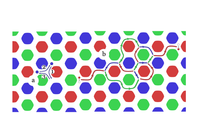
Figure 11: (color online) (a)A step by step illustration of hopping of two blue fermions with the net result of exchange of two fermions (b)A representation of a fermionic process in which a $c$-fermion (here red) at the origin site is annihilated and undergoes hopping, splitting and fusion processes, and then is created at another site.

Now we can think of constraints in (52) and (53) as a correlation between the low energy and high energy sectors of our model. They explicitly imply that the creation of a $c$-fermion creates the vortices with net topological charge of $({\bar{c}},\chi_{{\bar{\bar{c}}}})$. Alternatively, as suggested by mapping in (40), flipping of spin on a triangular can create or destroy the excitation, that is, a high energy fermion can be locally transformed into low energy ones. This amounts to attach a topological charge from low energy sector to high energy excitations. Thus a $c$-fermion carries a topological charge. On the other hand, an open $c$-string commutes with all plaquettes except some of them, so they create or destroy a particular charge among the charges in Fig.2. It is simple to check that which charge they carry at their open ends. In fact they carry $({\bar{\bar{c}}},\chi_{{\bar{c}}})$ charges. These latter charges have trivial mutual statistics relative to the charges carried by high energy fermions, since they belong to different families of fermions. Thus the charge carried by a $c$-string must be invisible to the high energy fermions.

V.2 Perturbative continuous unitary transformation

The physics behind Hamiltonian in (44) can be further explored by resorting to approximate methods. The specific form of the energy levels of our model in the isolated limit, the existence of equidistant levels, makes it suitable for perturbative continuous unitary transformations. In this method the Hamiltonian is replaced by an effective one within unitary transformations in which the resulting effective Hamiltonian preserves the total charges, i.e. $[H^{\mathrm{eff}},Q]=0$. Thus the analysis of the model relies on finding the effective Hamiltonian in a sector characterized by the number of charges at every order of perturbation. For our model each sector are determined by the number of $c$-fermions. Each term of the effective Hamiltonian in any sector is just a suitable combination of expressions in (46) in such a way that respects the total color charge in that sector. For now we briefly analyze the lowest charge sectors.

In the zero-charge sector, only the effective spin degrees of freedom do matter. The effective Hamiltonian is just a many-body Hamiltonian with terms that are product of plaquette operators as follows

$$H_{0}^{\mathrm{eff}}=E_{0}-\sum_{\{c\}}\sum_{\{f\}}O^{c_{1},...,c_{n}}_{f_{1},...,f_{n}}S^{c_{1}}_{f_{1}}...S^{c_{n}}_{f_{n}},$$ (56)

where the first and second sum run over an arbitrary collection of colors and plaquettes of effective honeycomb lattice. The coefficients $O$’s are determined at a given order of perturbation. The product of plaquette operators is nothing but the string-net operators. Let us focus at lowest order of perturbation, where the model represents non-interacting vortices. First, let us redefine plaquette operators as

$$B_{f}^{x}=j_{x}^{s/2}\prod_{v\in f}\tau_{v}^{x},\qquad B_{f}^{y}=j_{y}^{s/2}\prod_{v\in f}\tau_{v}^{y},$$ (57)

where $j_{w}:=J_{w}/|J_{w}|$. At ninth order of perturbation the effective Hamiltonian is

$$H^{\mathrm{eff}}_{0}=-\sum_{f\in\Lambda}\left(k_{x}B^{x}_{f}+k_{y}B^{y}_{f}+k_{z}B^{x}_{f}B^{y}_{f}\right),$$ (58)

with AnyonicFermions

$$k_{z}=\frac{3}{8}|J_{x}J_{y}|^{3}+O(J^{7}),~{}~{}~{}\frac{k_{x}}{|J_{y}|^{3}}=\frac{k_{y}}{|J_{x}|^{3}}=\frac{55489}{13824}{|J_{x}J_{y}|^{3}}.$$ (59)

This is exactly the many-body Hamiltonian of topological color code obtained in (34) using degenerate perturbation theory with the additional advantage of knowing the coefficients exactly. Its ground state is vortex free and can be written explicitly by choosing a reference state as

$$2^{N/4-1}\prod_{f}\left(\frac{1+B^{x}_{f}}{2}\right)|\Uparrow\rangle\otimes|0\rangle_{b}.$$ (60)

Other degenerate ground states can be constructed by considering the nontrivial string operators winding around the torus. Excitations above ground state don’t interact. Going to higher order of perturbation, as equation in (56) suggests, the ground states remain unchanged, however the excitation spectrum changes and vortices interact with each other.

The one-quasiparticle sector can also be treated by examining the expressions in (46). The effective Hamiltonian can be written as

$$H^{\mathrm{eff}}_{1}=H^{\mathrm{eff}}_{0}-\sum_{\{R\}}O_{R}\hat{R}b^{\dagger}_{c,R}b_{c}.$$ (61)

What the second term describes is nothing but the annihilation of a $c$-fermion at a reference site and then its creation at a site connected to the reference by a string-net $R$, as shown in Fig.11(b). Again notice that this string-net is just the product of green and red links of original 2-body Hamiltonian, in its effective form is given in terms of spin-boson degrees of freedom. The coefficients $O$’s are determined at any order of perturbation. Notice that these coefficients are different from those in (56). In the first order, only the hopping term does matter. Let us consider the sector containing a $c$-fermion. Up to this order, the fermion can only hop around a $c$-plaquette. This implies that at first order the fermion perform an orbital motion around a plaquette of its color. Notice that the fermion can not hop from a $c$-plaquette to other $c$-plaquette at the first order, since it needs for a composite process which appears at second order. This composite process is a combination of splitting and fusion processes. This is a virtual process in the sense that the splitting of a $c$-fermion into two ${\bar{c}}$- and ${\bar{\bar{c}}}$-fermion takes the model from 1-quasiparticle sector into the 2-quasiparticle sector, but the subsequent process fuses two particles into a single one turning back to 1-quasiparticle sector. Thus, at second order the $c$-fermion can jump from one orbit to other one.

At first order, for $J=J_{x}=J_{y}$, we get a $-2J$ contribution to the energy gap coming from orbital motion. Going to second order we get a non-flat dispersion relation. The gap, at this order, is given by $1-2J-J^{2}/2$ and thus it closes at $J\simeq 0.45$. This is just an approximate estimation, since we are omitting all fermion interactions and, perhaps more importantly, we are taking $J\simeq J_{z}$. However, it is to be expected that as the couplings $J_{x}\sim J_{y}$ grow in magnitude the gap for high-energy fermions will reduce, producing a phase transition when the gap closes. Such a phase transition resembles the anyon condensations discussed in family_non_Abelian ; nestedTO ; bais_slingerland09 . There are three topological charges invisible to the condensed anyons. This means that in the new phase there exists a residual topological order related to these charges. They have semionic mutual statistics underlying the topological degeneracy in the new phase.

V.3 Fermions and gauge fields

The emerging high-energy $c$-fermions always appear with some nontrivial gauge fieldsAnyonicFermions ; wen_statistics , and carry different representation of the gauge symmetry $\mathbf{Z}_{2}\times\mathbf{Z}_{2}$ of the model. Before clarifying this, we can see that the plaquette degrees of freedom correspond to $\mathbf{Z}_{2}\times\mathbf{Z}_{2}$ gauge fields. This correspondence is established via introducing the following plaquette operators

$$B_{f}^{\bar{\bar{c}}} :=j_{x}^{s/2}\,S_{f}^{\bar{c}},$$

$$B_{f}^{\bar{c}} :=j_{y}^{s/2}\,S_{f}^{\bar{\bar{c}}},$$

$$B_{f}^{c} :=(-j_{x}j_{y})^{s/2}\,S_{f}^{c}.$$ (62)

The gauge element $q_{f}\in\mathbf{Z}_{2}\times\mathbf{Z}_{2}$ that can be attached to the plaquette $f$ is determined by following eigenvalue conditions

$$\chi_{c}(q_{f})=B_{f}^{c},$$ (63)

which always has a solution due to

$$(B_{f}^{c})^{2}=B^{\mathrm{r}}_{f}B^{\mathrm{g}}_{f}B^{\mathrm{b}}_{f}=1.$$ (64)

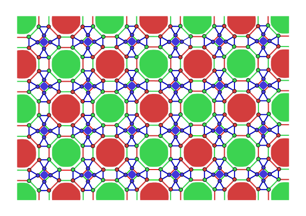
Figure 12: (color online) A piece of 2-body lattice corresponding to a 2-colex composed of octagon and square plaquettes. The lattice is 3-colorable as in Fig.8.

The ground state of color code Hamiltonian (58) is vortex free and corresponds to $\chi_{c}=1$. The fact that for a 2-colex with hexagonal plaquettes, the gauge fields can be related to representation of the group is immediate. One way to see this is to check the phase picked up by a $c$-fermion when it moves around a plaquette. Turning on a plaquette is done by combination of hopping operators yielding the phases as $B_{f}^{\bar{\bar{c}}}$, $B_{f}^{\bar{c}}$ and $B_{f}^{c}$ that are consistent with (64). However, this is not generic for all 2-colexes. For 2-colexe plaquettes that the number of their edges is a multiple of four, we see that the ground state carries fluxes. Perhaps the most important of such lattices is the so called 4-8-8 lattice shown in Fig.12. It contains inner octagons and squares. Once degenerate perturbation theory is applied about the strong limit of the system, the effective color code Hamiltonian in terms of plaquette operators in (V.3) at 12th order of perturbation is produced, as follows

$$H_{eff} = -\sum_{f}(k_{x}B_{f}^{x}+k_{y}B_{f}^{y}+k_{z}B_{f}^{z})+\mathrm{multiplaquette~{}terms},$$ (65)

where sum runs over all squares and octagons.

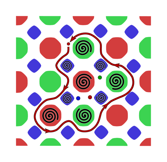
Figure 13: (color online) A $c$-fermion process. A red fermion goes around a region $\lambda$. The phase that it picks up depends on vortex configurations shown by spiral lines, blue and green fermions and number of plaquettes that the number of their edges is of multiple four.

Notice that at 12th order of perturbation multiplaquette terms that are product of square plaquette operators are also appeared. It is simple to check that the coefficients $k$’s have positive sign. As we can relate the plaquettes to the representation of gauge group, the ground state corresponds to vortex free sector. In fact, the ground state of all 2-colexes with plaquettes of any shape is vortex free and correspond to $\chi_{c}=1$ of gauge group. What is able to differentiate between ground states of 2-colex plaquttes with $4n$ ($n$ an integer) edges from others is related to the gauge fields attached to a fermion. In particular, there is a background of $\pi$-fluxes in the ground states of such lattices, and the emerging $c$-fermions can detect them. To make sense of the existence of such fluxes, let us consider a simple fermionic process as explained above. When a $c$-fermion turns on a plaquette, the combination of hopping terms yield $-B_{f}^{\bar{\bar{c}}}$, $-B_{f}^{\bar{c}}$ and $-B_{f}^{c}$, which clearly imply that

$$(-B_{f}^{\bar{\bar{c}}})(-B_{f}^{\bar{c}})(-B_{f}^{c})=-1.$$ (66)

This result exhibit that the ground states of color code models defined on lattices with $4n$-plaquettes carry fluxes. Thus, in its representation in terms of $\mathbf{Z}_{2}\times\mathbf{Z}_{2}$ gauge group, the fluxes must be subtracted away.

Our derivation for ground states with $0$- and $\pi$-flux can be compared with Lieb theoremlieb_flux , which states for a square lattice the energy is minimized by putting $\pi$ flux in each square face of the lattice. The connection to our models makes sense when we consider how 2-colexes with hexagonal and 4-8-8 plaquettes can be constructed from a square lattice by removing some edges. Then the total $\pi$ fluxes in a set of square faces corresponding to a 2-colex plaquette amounts to the flux that it carries. It is simple to see that each hexagonal plaquette composed of two (imaginary) square faces, and flux $\pi$ in each square face then implies flux $0$ in the hexagon. The same strategy holds for fluxes carried by the 4-8-8 plaquette(and in general for all $4n$-plaquettes). Once again we see that each plaquettes of latter 2-colxes is composed of odd number of square faces, thus they carry flux $\pi$ in their plaquettes.

Now we can give a general expression for the gauge fields seen by emerging high-energy fermions. To do so, let us consider a process in which a $c$-fermion is carried around a region $\lambda$, as in Fig.13. The hopping process yields a phase

$$\phi^{c}_{\lambda}=\chi_{c}(q_{\lambda})\,(-1)^{n_{\bar{c}}^{\lambda}+n_{\bar{\bar{c}}}^{\lambda}+n_{4}^{\lambda}}$$ (67)

where $q_{\lambda}=\prod_{\lambda}q_{f}$, $n_{c}^{\lambda}$ denotes the number of $c$-fermions inside $\lambda$ and $n_{4}^{\lambda}$ the number of 2-colex plaquettes inside $\lambda$ with a number of edges that is a multiple of four. Thus, we can see that each family of fermions carries a different representation of gauge group given by values of $q_{f}$ inside the region. Moreover, it emphasizes that fermions with different color charges have mutual semionic statistics. Clearly for hexagonal lattices $n_{4}^{\lambda}=0$, and the ground state carries no fluxes.

VI Fermionic Mapping

In this section we will come back to the original Hamiltonian of (6) on the lattice in order to use another approximate method based on fermionic mappings. This Hamiltonian can be fermionized by Jordan-Wigner transformation Feng_et_al07 . To do so, firstly it is convenient to present a lattice which is topologically equivalent to the lattice of Fig.3. This is a new type of ”brick-wall” lattice as shown in Fig.14. The black and white sites are chosen such that, at the effective level, the lattice be a bipartite lattice, since the effective spins are located at the vertices of hexagonal lattice representing a bipartite lattice. Note that neither original lattice in Fig.3 nor the brick-wall one in Fig.14 are bipartite in their own. Also as we will see, the fermionization of the model needs some ordering of sites in the ”brick-wall” lattice. The unit cell of the brick-wall lattice is comprised of two triangles as shown in Fig.14 in a yellow ellipse. The translation vectors $\vec{n}_{1}$ and $\vec{n}_{2}$ connect different unit cells of the lattice.

The deformation of the original lattice into a ”brick-wall” lattice allows one to perform the one dimensional Jordan-Wigner transformation. The one dimensional structure of the lattice is considered as an array of sites on a contour as shown in Fig.15. The sites on the contour can be labeled by a single index and the ordering of the sites is identified by the direction of the arrows in Fig.15. The expression of the Pauli operators in terms of spinless fermions will be:

$$\sigma^{+}_{j}=a^{{\dagger}}_{j}\exp\left(i\pi\sum_{l<j}a^{{\dagger}}_{l}a_{l}\right),~{}~{}~{}\sigma^{z}_{j}=(2a^{{\dagger}}_{j}a_{j}-1),$$ (68)

where spinless fermions satisfy the usual anticommutation relations as follows

$$\{a_{i},a^{\dagger}_{j}\}=\delta_{ij},~{}~{}\{a^{\dagger}_{i},a^{\dagger}_{j}\}=\{a_{i},a_{j}\}=0.$$ (69)

Next, we introduce Majorana fermions as follows:

$$c_{j}=-i(a^{{\dagger}}_{j}-a_{j}),~{}~{}~{}d_{j}=a^{{\dagger}}_{j}+a_{j}$$ (70)

for black sites and

$$c_{j}=a^{{\dagger}}_{j}+a_{j},~{}~{}~{}d_{j}=-i(a^{{\dagger}}_{j}-a_{j})$$ (71)

for white sites. Majorana operators are Hermitian and satisfy the following relations:

$$k^{2}_{j}=1,~{}~{}~{}k_{j}k_{i}=-k_{i}k_{j}~{}~{}~{}i\neq j,$$ (72)

where $k=c,d$.

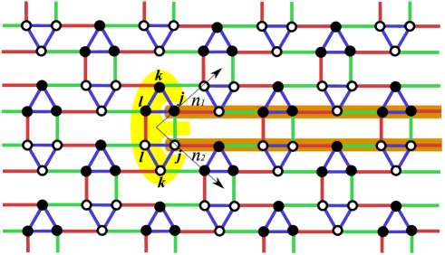
Figure 14: (color online) Brick-wall lattice that is topologocally equivalent to the original lattice in Fig.3. Triangles with black and white vertices are chosen such that at the logical level they correspond to a bipartite lattice. A unit cell of the lattice has been shown by yellow region and the whole lattice can be constructed by translation vectors $\mathbf{n_{1}}$ and $\mathbf{n_{2}}$. The chains supporting the field operator $F$ have been shown by brown ribbons.

For each unit cell we can realize two vertical red and green links corresponding to $\sigma^{x}\sigma^{x}$ and $\sigma^{y}\sigma^{y}$ interactions. Observe that each vertex of the lattice can be specified by three indices as follows: (i) index $\mathrm{I}$ is introduced to specify which unite cell the vertex belongs to, (ii) $\mathrm{b}$ ($\mathrm{w}$) denotes the black (white) vertex, (iii) $l$, $j$ or $k$ label the position of the vertex in each triangle. With this labeling of vertices, the expression of the different terms appearing in the two-body Hamiltonian in terms of Majorana fermions is listed below:

$$\mathrm{blue~{}links}:~{}\sigma^{z}_{j}\sigma^{z}_{k}=i\hat{U}_{jk}d_{j}d_{k},$$

$$\mathrm{horizontal~{}r-links}:~{}\sigma^{x}_{j}\sigma^{x}_{k}=id_{j}d_{k},$$

$$\mathrm{horizontal~{}g-links}:~{}\sigma^{y}_{j}\sigma^{y}_{k}=-id_{j}d_{k},$$

$$\mathrm{vertical~{}r-links}:~{}\sigma^{(\mathrm{Iw})x}_{l}\sigma^{(\mathrm{Ib})x}_{l}=id^{(\mathrm{Iw})}_{l}d^{(\mathrm{Ib})}_{l}\hat{F}_{\mathrm{I}},$$

$$\mathrm{vertical~{}g-links}:~{}\sigma^{(\mathrm{Iw})y}_{j}\sigma^{(\mathrm{Ib})y}_{j}=-id^{(\mathrm{Iw})}_{j}d^{(\mathrm{Ib})}_{j}\hat{F}_{\mathrm{I}},$$ (73)

where $\hat{U}_{jk}=-ic_{j}c_{k}$ and the operator $\hat{F}_{\mathrm{I}}$ is a non-local operator. Interestingly enough, this non-local term has the following expression:

$$\hat{F}_{\mathrm{I}}=\exp(i\pi\sum^{k-1}_{l=j}a^{{\dagger}}_{l}a_{l})=\prod_{l\in R}ic_{l}d_{l},$$ (74)

where we have used the ordering of the brick-wall lattice and $R$ stands for a set of spins crossed by two brown ribbons shown in Fig.14.

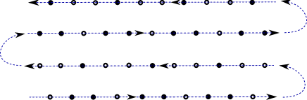
Figure 15: (color online) Ordering of sites in the brick-wall lattice of Fig.14. Such ordering makes it possible to perform a one-dimensional Jordan-Wigner transformation.

Observe that for each unit cell we can realize such ribbons. The non-local operator can be written as a product of some plaquette operators each corresponding to a rectangle(inner hexagon) wrapped by the ribbons. Notice that an inner hexagon of the ruby lattice in Fig.3 looks like a rectangle in the brick-wall lattice. Thus, two ribbons are nothing but a combination of rectangles as in Fig.14. This plaquette operator precisely corresponds to operator $S^{C}_{f}$ in Fig.5. Let $f_{1},f_{2},...$ stand for those rectangles (inner hexagons). Thus, we have:

$$\hat{F}_{\mathrm{I}}=\prod_{l\in R}c_{l}d_{l}=S^{C}_{f_{1}}\otimes S^{C}_{f_{2}}\otimes S^{C}_{f_{3}}....$$ (75)

After all these transformations, we arrive at an exact fermionized Hamiltonian given by

$$H = -J_{z}\sum_{b-link}i\hat{U}_{jk}d_{j}d_{k}-J_{x}\sum_{r-link}id_{j}d_{k}+J_{y}\sum_{g-link}id_{j}d_{k}$$ (76)

$$-J_{x}\sum_{\mathrm{I}}id^{(\mathrm{Iw})}_{l}d^{(\mathrm{Ib})}_{l}\hat{F_{\mathrm{I}}}+J_{y}\sum_{\mathrm{I}}id^{(\mathrm{Iw})}_{j}d^{(\mathrm{Ib})}_{j}\hat{F}_{\mathrm{I}}.$$

It is simple to check the following commutation relations:

$$\left[H,\hat{F}_{{}_{I}}\right]=\left[H,\hat{U}_{jk}\right]=\left[\hat{F}_{\mathrm{I}},\hat{F}_{\mathrm{I}^{\prime}}\right]=0.$$ (77)

Since $\hat{F}_{\mathrm{I}}^{2}=1$, the nonlocal operators can be replaced by its eigenvalues $F_{\mathrm{I}}=\pm 1$ . Thus the nonlocal terms appearing in the Hamiltonian which are related to the vertical links of the brick-wall lattice can be reduced to quadratic terms. However, the first sum in (76) which is related to the triangles cannot be reduced to the quadratic term. This is because local fields $\hat{U}_{jk}$ corresponding to three links of a triangle anticommute with each other as well as with some $\hat{F}_{\mathrm{I}}$’s. Due to these anticommutation, all fields cannot be fixed independently. This fact is in sharp contrast with Kitaev’s model and its variants. These latter models are defined on trivalent lattices. The different fields live at spatially separated links allowing a free fermion exact solution honeycomb ; Feng_et_al07 . The obtained quadratic Hamiltonian describes free majorana fermions in a background of $\mathbf{Z}_{2}$ charges. Instead, the lattice of our model is 4-valent, a sharp difference that prevents complete solvability and gives rise to very interesting features not present in the mentioned models. Note that the fields $\hat{U}_{jk}$ are highly interacting since on a triangle three fields go to vacuum in the sense that $\hat{U}_{jk}\hat{U}_{kl}\hat{U}_{lj}=-1$. This is resemblance of vertex interaction in high energy fermions that we have seen in Sect.V with the bosonic mapping. However, this latter relation doesn’t coincide with the symmetry of the model as they do not commute with each other. This will be considered next.

Thus far, we have considered fields that are present in the Hamiltonian. In what follows, we introduce another set of fields which have the $\mathbf{Z}_{2}\times\mathbf{Z}_{2}$ symmetry commuting with each other and with the Hamiltonian. To this end, consider a plaquette $f$. As before, by a plaquette we mean an outer and an inner hexagon with six triangles between them. Let $V_{f}$ and $V_{h}$ stand for sets of vertices of plaquette and inner hexagon, respectively. It is natural that $V_{h}\subset V_{f}$. To each plaquette we attach the three following fields:

$$\phi^{1}_{f}=\prod_{j\in V_{f}}c_{j},~{}\phi^{2}_{f}=\prod_{j\in f\backslash h}c_{j}\prod_{v\in V_{h}}d_{j},~{}\phi^{3}_{f}=\prod_{j\in V_{h}}c_{j}d_{j},$$ (78)

where by $f\backslash h$ we simply mean $V_{f}-V_{h}$. Each $\phi_{f}$ squares identity. They commute with each other and with Hamiltonian and $\hat{F_{\mathrm{I}}}$:

$$\left[\phi^{k}_{f},\phi^{k^{\prime}}_{f^{\prime}}\right]=\left[\phi^{k}_{f},\hat{F}_{\mathrm{I}}\right]=\left[H,\phi^{k}_{f}\right]=0$$ (79)

Also, the fields $\phi_{f}$ are responsible of the $\mathbf{Z}_{2}\times\mathbf{Z}_{2}$ gauge symmetry since $\phi^{1}_{f}\otimes\phi^{2}_{f}\otimes\phi^{3}_{f}=-1$. The above fields are related to the plaquette operators.Using the transformations we have introduced in (VI), we can fermionize the conserved plaquette operators obtained in Fig.5. They are associated to the above constants of motion as follows

$$S^{A}_{f}=\phi^{1}_{f}\hat{F}_{\mathrm{I}},~{}~{}~{}S^{B}_{f}=\phi^{2}_{f}\hat{F}_{\mathrm{I}},~{}~{}~{}S^{C}_{f}=\phi^{3}_{f}.$$ (80)

Although the above gauge fields make it possible to divide the Hilbert space into sectors in which be eigenspaces of gauge fields (or eigenspaces of plaquette operators), they do not allow us to reduce the Hamiltonian in (76) into a quadratic form. The $\hat{F}_{\mathrm{I}}$’s can be fixed as they commute with the Hamiltonian. But, we are not able to reduce the four-body interaction terms in the Hamiltonian into quadratic form. In fact, the anticommutation of $\hat{U}_{jk}$’s on a blue triangle prevents them to be fixed consistently with gauge fixing.

VII Conclusions

We have introduced a two-body spin-1/2 model in a ruby lattice, see Fig.3. The model exhibits an exact topological degeneracy in all coupling regimes. The connection to the topological color codes can be discussed on the non-perturbative level as well as confirmed by perturbative methods. In the former case, on the ruby lattice we realized plaquette operators with local $\mathbf{Z}_{2}\times\mathbf{Z}_{2}$ symmetry of the color codes. All plaquette operators commute with the Hamiltonian and they correspond to integrals of motion. The plaquettes can be extended to more complex objects that can be considered as string-nets: non-trivial strings with branching points. The nontrivial strings corresponding to the various homology classes of the manifold determine the exact degeneracy of the model. For the case of periodic boundary conditions, i.e on a torus, and for each non-contractible cycle of the torus, we can identify three nontrivial closed strings. Once each of them is colored, the plaquettes of the lattice can be correspondingly colored as in Fig.8. For each homology class, they are related to each other by the gauge symmetry of the model. The crucial property of these strings is that they commute with Hamiltonian but not always with each other. This is independent of the regimes of coupling constants of the model. Being anticommuting closed nontrivial strings, the model has exact topological degeneracy. To clarify this observation, we use perturbation theory to investigate a regime of coupling corresponding to a strong coupling limit (triangular limit). In this limit the topological color code will be the effective description of the model. The effective representation of the closed loop operators determine the terms appearing in the effective Hamiltonian at different orders.

Unlike the Kitaev’s model or any its variants, our model is not integrable in terms of mapping to Majorana fermions, to the best of our knowledge. This model is a four-valent lattice and gauge fields not always commute with each other. However, we have emphasized in Sect.III that the existence of exact integrals of motion (IOMs) at a non-perturbative level is far more enriching than demanding exact-solvability of a model. In fact, if the number of IOMs is large enough, the model can turn out to be solvable. Thus, fixing plaquette operators can not give rise to fix all gauge fields.

The description of our model in terms of hard core bosons yields very fruitful and interesting physics of the model. Using a bosonic mapping, it is possible to discuss the emergence of strongly interacting anyonic fermions. They form three classes each of one color. Fermions from different classes have mutual semionic statistics. A very intriguing feature of these fermions is related to the topological color charges they carry. They carry charges from a particular family of low energy fermions. Thus the charges created by open strings are invisible to high energy fermions. Moreover, there are some experimental proposals to realize hard-core bosons with optical latticesexperiment_hardcore and it would be a nice challenge to implement a Hamiltonian like (44) and (45).

We have shown that this new model exhibits enough novel interesting and relevant properties so as to justify further research. Some of these possible lines of study are as follows: We have only studied a particular phase of the system, although we are able to study non-perturbative effects as well. The fact that all phases show a topological degeneracy anticipates a rich phase diagram. In this regard, one may explicitly break the color symmetry that the model exhibits and still keep the features that we have discussed. It would be particularly interesting to check whether any of the phases displays non-abelian anyons. The model has many integrals of motion, although not enough to make it exactly solvable. This becomes another appealing feature of the model since other methods of study, like numerical simulations and experimental realizations will help to give a complete understanding of all its phases.

Acknowledgements We acknowledge financial support from a PFI grant of EJ-GV, DGS grants under contracts, FIS2006-04885, and the ESF INSTANS 2005-10.

Appendix A 2-Body Hamiltonian for Color Codes using Cluster States

A topological color code can be constructed from a graph state defined on a bipartite lattice by means of a set of measurements on certain subsystems. This bipartite lattice is shown in Fig.16(a), where the black vertices correspond to plaquettes and the white vertices correspond to the vertices of a 2-colex. To this graph we can attach a set of stabilizers as follows

$$K_{\alpha}=X_{\alpha}\prod_{\prec\alpha,\beta\succ}Z_{\beta},$$ (81)

where $\alpha$ and $\beta$ stand for vertices of the graph and the product runs over all vertices that are connected to $\alpha$ by black links. Let us set $V=\mathfrak{U}_{1}\cup\mathfrak{U}_{2}$, where $\mathfrak{U}_{1}$ and $\mathfrak{U}_{2}$ stand for the set of white and black vertices of the bipartite graph in Fig.16(a). Note that white and black vertices corresponds to the vertices and plaquettes of the 2-colex. This bipartite graph is exactly what we need to construct color codes. To this end, we first impose a unitary transformation on the sublattices that allows us to have a more symmetric form of the stabilizer operators, i.e

$$\forall~{}~{}v\in\mathfrak{U}_{1}~{}~{}~{}~{}~{}K_{v}=X_{N(v)}$$

$$\forall~{}~{}f\in\mathfrak{U}_{2}~{}~{}~{}~{}~{}K_{f}=Z_{N(f)},$$ (82)

where $N(v)$ denotes the site $v$ and its neighbors, and the same goes for $N(f)$. The corresponding cluster state denoted by $|G\rangle$ will be the common eigenvector of the above stabilizer operators. Thus we have:

$$\forall~{}~{}v\in\mathfrak{U}_{1}~{}~{}~{}~{}~{}X_{N(v)}|G\rangle=|G\rangle$$

$$\forall~{}~{}f\in\mathfrak{U}_{2}~{}~{}~{}~{}~{}Z_{N(f)}|G\rangle=|G\rangle.$$ (83)

Finally, a graph state can be related to a color code within a set of measurements in the $Z$ basis on all qubits corresponding to the set $\mathfrak{U}_{2}$.

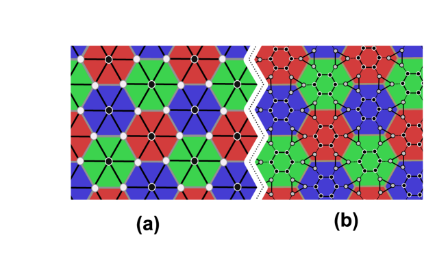
Figure 16: (color online) (a) The graph needed for obtaining color codes from graph states. The graph is bipartite. Black and white vertices correspond to the plaquettes and vertices of a 2-colex. Black solid links are edges of the graph (b) The corresponding graph state can be approximated as a low energy description of a lattice with 2-body Hamiltonian. The lattice is obtained from the graph by replacing its vertices with some hexagons and triangles. The interactions $\sigma^{z}\sigma^{z}$ and $\sigma^{x}\sigma^{z}$ are associated to the solid and dashed links, respectively.

We suppose there is a two dimensional lattice of physical qubits that is governed by a 2-body Hamiltonian. Physical qubits of the lattice are projected to logical qubits. The point is that this projection is achieved by going to some order in perturbation theory. We think of vertices of the graph in Fig.16(a) as logical qubits. The lattice with 2-body interaction is shown in Fig.16(b), where the number of physical qubits corresponding to the vertices of the graph equals the number of links crossing the vertex. The new resulting lattice consists of triangles and hexagons and physical qubits live on their vertices. Triangles and hexagons are in one to one correspondence with the white and black vertices ($\mathfrak{U}_{1}$ and $\mathfrak{U}_{2}$) of the graph in Fig.16(b), respectively. Note that each triangle is linked with three neighboring hexagons and each hexagon is linked with six neighboring triangles.

The low lying spectrum of a well constructed 2-body Hamiltonian defined on the lattice composed of hexagons and triangles may describe a cluster state. To this end, we need for the following projection from the physical qubits to the logical ones:

$$P_{v}=|\!\Uparrow_{v}\rangle\langle\uparrow\uparrow\uparrow\!|+|\!\Downarrow_{v}\rangle\langle\downarrow\downarrow\downarrow\!|,~{}~{}P_{f}=|\!\Uparrow_{f}\rangle\langle\uparrow\uparrow\uparrow\uparrow\uparrow\uparrow\!|+|\!\Downarrow_{f}\rangle\langle\downarrow\downarrow\downarrow\downarrow\downarrow\downarrow\!|$$ (84)

where $|\!\Uparrow_{L}\rangle$ and $|\!\Downarrow_{L}\rangle$ with $L=v,f$ stand for the two states of the logical qubits obtained within the above projections, or alternatively they are states of logical qubits of the graph in Fig.16(a). We set the following Hamiltonian:

$$H=H_{0}+\lambda V$$ (85)

where $H_{0}$ is the unperturbed Hamiltonian which can be treated exactly and $\lambda$ is a small quantity which allow us to treat the term $\lambda V$ perturbatively. We refer to each triangle (hexagon) and its vertices by a site index $v$ ($f$) and indices $i,j$, respectively. The unperturbed part of the Hamiltonian included in $H_{0}$ is as follows.

$$H_{0}=-\sum_{L}\sum_{<i,j>}\sigma^{z}_{L,i}\sigma^{z}_{L,j}$$ (86)

where the first sum runs over all triangles and hexagons (sites) and $<\!\!i,j\!\!>$ stand for the nearest-neighbor qubits around the corresponding triangle or hexagon connected by the solid lines as in the Fig.16(b). The interaction between qubits of triangles and qubits of hexagons are included in $V$:

$$V=-\sum_{<vi,fj>}(\sigma^{x}_{v,i}\sigma^{z}_{f,j}+\sigma^{z}_{v,i}\sigma^{x}_{f,j})$$ (87)

where $<\!\!vi,fj\!\!>$ denotes two neighboring qubits which are connected by the dashed line. The unperturbed Hamiltonian $H_{0}$ can easily be diagonalized for triangles and hexagons. Ground state vectors of a triangle or hexagon form a two dimensional space spanned by the following polarized eigenvectors:

$$\mathrm{triangle:}~{}~{}|\!\Uparrow_{v}\rangle\equiv|\!\uparrow\uparrow\uparrow\rangle,~{}~{}~{}|\!\Downarrow_{v}\rangle\equiv|\!\downarrow\downarrow\downarrow\rangle$$ (88)

and

$$\mathrm{hexagon:}~{}~{}|\!\Uparrow_{f}\rangle\equiv|\!\uparrow\uparrow\uparrow\uparrow\uparrow\uparrow\rangle,~{}~{}~{}|\!\Downarrow_{f}\rangle\equiv|\!\downarrow\downarrow\downarrow\downarrow\downarrow\downarrow\rangle.$$ (89)

Let $N_{v}$ and $N_{f}$ be the number of triangles and hexagons, respectively. Imposing periodic boundary conditions, the total number of triangles and hexagons will be: $N=N_{v}+N_{f}=3N_{f}$ . Thus, the dimension of the ground-space of the unperturbed Hamiltonian $H_{0}$ (or ground state degeneracy) becomes: $g_{0}=2^{N_{v}}2^{N_{f}}=2^{N}$, and the ground state energy is: $E_{0}^{(0)}=N_{f}(-6)+N_{v}(-3)=-4N$ in terms of the energy scale of the problem. The first excited state is produced by exciting one of the triangles or hexagons and has energy: $E_{1}^{(0)}=N_{f}(-6)+N_{v}(-3)+4=-4(N-1)$ with degeneracy $g_{1}=14N2^{N}$. The second excited state has energy $E_{1}^{(0)}=N_{f}(-6)+N_{v}(-3)+8=-4(N-2)$ with degeneracy: $g_{2}=4(N+5N^{2})2^{N-1}$, and so on and so forth.

Using degenerate perturbation theory as in Sec.IV.2, the effect of perturbation $V$ on the ground sate subspace can be investigated, and see if it breaks the degeneracy. It is simple to see that first order perturbation does not have anything to do with the ground state subspace. The second order gives rise to a trivial effect as a shift in energy, since each operator related to dashed links appears twice. The third order perturbation theory however gives rise to a nontrivial effect. It causes a partial lift of the ground state degeneracy, but not complete. The initial degeneracy $2^{N}$ gets reduced down to $2^{N_{f}}$. This nontrivial effect arises from the product of three dashed links crossing a typical triangle, namely the ground state vectors are grouped into the $2^{N_{v}}$ states, each containing $2^{N_{f}}$ vectors. The product of three (six) $\sigma^{x}$ operators around a triangle (hexagon) is equivalent to an $X$ operator acting on the logical qubit which is projected down from the three(six) qubits of the triangle(hexagon) , since

$$X_{L}=|\!\Uparrow_{L}\rangle\langle\Downarrow_{L}\!|+|\!\Downarrow_{L}\rangle\langle\Uparrow_{L}\!|.$$ (90)

Also the action of a $\sigma^{z}$ on one qubit of a triangle or hexagon is equivalent to an $Z$ operator acting on the related logical qubit, since

$$Z_{L}=P_{L}\sigma^{z}P^{\dagger}_{L}=|\!\Uparrow_{L}\rangle\langle\Uparrow_{L}\!|-|\!\Downarrow_{L}\rangle\langle\Downarrow_{L}\!|.$$ (91)

Now we can go on in order to calculate the third order perturbation:

$$H^{(3)}_{\mathrm{eff}}=-\frac{3!}{(E^{(0)}_{0}-E^{(0)}_{1})^{2}}\sum_{v}K_{v}=-\delta\sum_{v}K_{v},$$ (92)

where

$$K_{v}=X_{v}\prod_{f}Z_{f},$$ (93)

the product runs over three black vertices linked to the $v$ and $\delta=\frac{3}{8}$. The operator $K_{v}$ is a stabilizer for the logical qubits which are projected down from the triangles. Since $K_{v}^{2}=1$, the ground states correspond to the values of $k_{v}=+1$. We skip the forth and fifth order of perturbation because they have trivial effects.

Like in $3^{rd}$ order perturbation, we are faced with a nontrivial term in the $6^{th}$ order perturbation theory. We will see that by considering this order, the ground state degeneracy is lifted completely. This nontrivial effect arises from the product of terms in the perturbation $\lambda V$ corresponding to the links around a hexagon. Finally, for the $6^{th}$ order perturbation we have:

$$H^{(6)}_{\mathrm{eff}}=-\gamma\sum_{f}K_{f},$$ (94)

where

$$K_{f}=X_{f}\prod_{v}Z_{v},$$ (95)

and the product runs over six white vertices linked to the hexagon $f$. The coefficient $\gamma$ has positive sign and its precise value is unimportant. We would like to emphasize that at six order in perturbation theory some other terms appear which are product of two distinct $K_{v}$. However, we skip them as they all commute. Equations (93) and (95) provides all we need to adopt the cluster state in (83) as ground state of the low energy effective theory of Hamiltonian in (85), which up to six order of perturbation can be written as follows

$$H_{\mathrm{eff}}=\mathrm{constant}-\delta\sum_{v}K_{v}-\gamma\sum_{f}K_{f}.$$ (96)

We see that the above effective Hamiltonian is completely different from that of in (34). The latter equation gives rise directly to the topological color code as its ground state, but the ground state (cluster state) of former one needs further local measurements to encode the desired color code.

References

References

- (1) H. Bombin, M. A. Martin-Delgado; “Topological Quantum Distillation”; Phys. Rev. Lett. 97, 180501 (2006); quant-ph/0605138.
- (2) H. Bombin, M.A. Martin-Delgado; “Topological Computation without Braiding”; Phys. Rev. Lett. 98, 160502 (2007); quant-ph/0610024.
- (3) H. Bombin, M.A. Martin-Delgado “Exact Topological Quantum Order in D=3 and Beyond: Branyons and Brane-Net Condensates”; Phys. Rev. B 75, 075103 (2007); cond-mat/0607736.
- (4) H. J. Briegel, R. Raussendorf, Phys. Rev. Lett. 86, 910 (2001).
- (5) R. Raussendorf, H. J. Briegel, Phys. Rev. Lett. 86, 5188 (2001); Quantum Inf. Comput. 2, 443 (2002).
- (6) R. Raussendorf, D. E. Browne, and H. J. Briegel, Phys. Rev. A 68, 022312 (2003).
- (7) H. Bombin, M.A. Martin-Delgado, “Statistical mechanical models and topological color codes”; Physical Review A 77, 042322 (2008). arXiv:0711.0468.
- (8) S. D. Bartlett and T. Rudolph, Phys. Rev. A 74, 040302(R) (2006).
- (9) M. Van den Nest, K. Luttmer, W. Dür and H. J. Briegel, Phys. Rev. A 77, 012301 (2008).
- (10) H. Bombin, M. Kargarian, M.A. Martin-Delgado, “Interacting Anyonic Fermions in a Two-Body ‘Color Code’ Model”; Phys. Rev. B 80, 075111 (2009). arXiv:0811.0911.
- (11) M. Nielsen and I. Chuang, Quantum Computation and Quantum Information (Cambridge University Press, Cambridge, England, 2000).
- (12) A. Galindo and M. A. Martin-Delgado, Information and Computation: Classical and Quantum Aspects; Rev. Mod. Phys. 74, 347 (2002). Electronic preprint arXiv:quant-ph/0112105.
- (13) J.E. Levy, A. Ganti, C.A. Phillips, B.R. Hamlet, A.J. Landahl, T.M. Gurrieri, R.D. Carr, M.S. Carroll, “The impact of classical electronics constraints on a solid-state logical qubit memory”; arXiv:0904.0003.
- (14) A. Micheli, G.K. Brennen, P. Zoller, “A toolbox for lattice spin models with polar molecules”; Nat. Phys. 2, 341 (2006). quant-ph/0512222.
- (15) L. Jiang, G.K. Brennen, A.V. Gorshkov, K. Hammerer, M. Hafezi, E. Demler, M.D. Lukin, P. Zoller, “Anyonic interferometry and protected memories in atomic spin lattices”; Nat. Phys. 4, 482 (2008). arXiv:0711.1365.
- (16) M. Müller, L. Liang, I. Lesanovsky, P. Zoller, “Trapped Rydberg ions: from spin chains to fast quantum gates”; New J. of Phys. 10, 093009 (2008). arXiv:0709.2849
- (17) L.-M. Duan, E. Demler, M.D. Lukin, “Controlling Spin Exchange Interactions of Ultracold Atoms in Optical Lattices”; Phys. Rev. Lett. 91, 090402 (2003). arXiv:cond-mat/0210564.
- (18) J.J. Garcia-Ripoll, M.A. Martin-Delgado, J.I. Cirac, “Implementation of Spin Hamiltonians in Optical Lattices”; Phys. Rev. Lett. 93, 250405 (2004).
- (19) M.J. Hartmann, F.G.S.L. Brandao, M.B. Plenio, “Strongly interacting polaritons in coupled arrays of cavities”; Nat. Phys. 2, 849 (2006). quant-ph/0606097.
- (20) M. Lewenstein, A. Sanpera, V. Ahufinger, B. Damski, A. Sen, U. Sen, “Ultracold atomic gases in optical lattices: mimicking condensed matter physics and beyond”; Adv. Phys. 56, 243 (2007).
- (21) J. Du, J. Zhu, M. Shi, X. Peng, D. Suter, “Experimental observation of a topological phase in the maximally entangled state of a pair of qubits”; Phys. Rev. A 76, 042121 (2007). arXiv:0705.3566.
- (22) A.F. Albuquerque, H.G. Katzgraber, M. Troyer, G. Blatter, “Engineering exotic phases for topologically protected quantum computation by emulating quantum dimer models”; Phys. Rev. B 78, 014503 (2008).
- (23) G.K. Brennen, M. Aguado, J.I. Cirac, “Simulations of quantum double models”; arXiv:0901.1345.
- (24) F. Wilczek, “Quantum Mechanics of Fractional-Spin Particles”. Phys. Rev. Lett. 49, 957 (1982).
- (25) J.M. Leinaas, J. Myrheim, “On the theory of identical particles”. Il Nuovo Cimento B37, 1 (1977).
- (26) G. Moore, N. Read, “Nonabelions in the fractional quantum Hall effect”, Nucl. Phys. B 360, 362 (1991).
- (27) X.G. Wen, Quantum Field Theory of Many-body Systems: From the Origin of Sound to an Origin of Light and Electrons (Oxford Univ. Press, New York, 2004).
- (28) X.G. Wen, “Topological orders and edge excitations in fractional quantum Hall states”; Adv. Phys., 44, 405 (1995).
- (29) H. Bombin, M.A. Martin-Delgado, “Interferometry-free protocol for demonstrating topological order”; Physical Review B 78, 165128 (2008). arXiv:0705.0007.
- (30) D. Gottesman, “Class of quantum error-correcting codes saturating the quantum Hamming bound”. Phys. Rev. A 54, 1862 (1996).
- (31) Z.W.E. Evans, A.M. Stephens, “Optimal decoding in fault-tolerant concatenated quantum error correction”; arXiv:0902.4506.
- (32) Z.W.E. Evans, A.M. Stephens, “Accuracy threshold for concatenated error detection in one dimension”; arXiv:0902.2658.
- (33) A. Yu. Kitaev, “Fault-tolerant quantum computation by anyons”, Annals of Physics 303, 2 (2003). quant-ph/9707021.
- (34) H. Bombin, M.A. Martin-Delgado; “Homological Error Correction: Classical and Quantum Codes”; J. Math. Phys. 48, 052105 (2007); quant-ph/0605094.
- (35) H. Bombin, M.A. Martin-Delgado; “Topological quantum error correction with optimal encoding rate”; Physical Review A 73, 062303 (2006). quant-ph/0602063.
- (36) C.D. Albuquerque, R. Palazzo, E.B. Silva, “Topological quantum codes on compact surfaces with genus ”; J. Math. Phys. 50, 023513 (2009).
- (37) S. Bullock, G.K. Brennen, “Qudit surface codes and gauge theory with finite cyclic groups”; J. of Phys. A: Math. and Theor. 40, 3481 (2007).
- (38) H. Bombin, M.A. Martin-Delgado; “Optimal Resources for Topological 2D Stabilizer Codes: Comparative Study”, Phys. Rev. A 76, 012305 (2007). quant-ph/0703272.
- (39) M. Planat, M.R. Kibler, “Unitary reflection groups for quantum fault tolerance”; arXiv:0807.3650.
- (40) L.S. Georgiev, “Computational equivalence of the two inequivalent spinor representations of the braid group in the topological quantum computer based on Ising anyons”; arXiv:0812.2337.
- (41) D. Hu, W. Tang, M. Zhao, Q. Chen, S. Yu, C.H. Oh, “Graphical nonbinary quantum error-correcting codes”; Phys. Rev. A 78, 012306 (2008). arXiv:0801.0831.
- (42) L.S. Georgiev, “Towards a universal set of topologically protected gates for quantum computation with Pfaffian qubits”; Nuc. Phys. B 789, 552 (2008).
- (43) H. Bombin, M.A. Martin-Delgado; “Quantum measurements and gates by code deformation”; J. of Phys. A: Math. and Theor. 42, 095302 (2009). arXiv:0704.2540.
- (44) R. Raussendorf, J. Harrington, K. Goyal, “Topological fault-tolerance in cluster state quantum computation”; New J. of Phys. 9, 199 (2007). arXiv:quant-ph/0703143.
- (45) R. Raussendorf, J. Harrington, “Fault-Tolerant Quantum Computation with High Threshold in Two Dimensions”; Phys. Rev. Lett. 98, 190504 (2007). quant-ph/0610082.
- (46) D. P. DiVincenzo, “Fault tolerant architectures for superconducting qubits”; arXiv:0905.4839.
- (47) E. Dennis, A. Kitaev, A. Landahl, J. Preskill, “Topological quantum memory”. J. Math. Phys. 43, 4452-4505 (2002).
- (48) H.G. Katzgraber, H. Bombin, M.A. Martin-Delgado, “Error Threshold for Color Codes and Random 3-Body Ising Models”; Phys. Rev. Lett. 103, 090501 (2009). arXiv:0902.4845.
- (49) M. Ohzeki, “Threshold of topological color code”; arXiv:0903.2102.
- (50) W.-B. Gao, A.G. Fowler, R. Raussendorf, X.-C. Yao, H. Lu, P. Xu, C.-Y. Lu, C.-Z. Peng, Y. Deng, Z.-B. Chen, J.-W. Pan; “Experimental demonstration of topological error correction”. arXiv:0905.1542v2.
- (51) R. Alicki, M. Fannes, M. Horodecki, “A statistical mechanics view on Kitaev’s proposal for quantum memories”, J. Phys. A: Math. Theor. 40 (2007) 6451-6467.
- (52) R. Alicki, M. Fannes, M. Horodecki, “On thermalization in Kitaev’s 2D model”; arXiv:0810.4584.
- (53) R. Alicki, M. Horodecki, P. Horodecki, R. Horodecki, “On thermal stability of topological qubit in Kitaev’s 4D model”; arXiv:0811.0033.
- (54) S. Iblisdir, D. Perez-Garcia, M. Aguado, J. Pachos, “Thermal States of Anyonic Systems”; arXiv:0812.4975.
- (55) S. Iblisdir, D. Perez-Garcia, M. Aguado, J. Pachos, “Scaling law for topologically ordered systems at finite temperature”; arXiv:0806.1853.
- (56) S. Bravyi, B. Terhal, “A no-go theorem for a two-dimensional self-correcting quantum memory based on stabilizer codes”; arXiv:0810.1983.
- (57) M. Kargarian, “Finite temperature topological order in 2D topological color codes”; Physical Review A 80, 012321 (2009). arXiv:0904.4492.
- (58) M. Kargarian, “Entanglement properties of topological color codes”; Physical Review A 78, 062312 (2008). arXiv:0809.4276.
- (59) H-H. Tu, G-M. Zhang, T. Xiang, Z-X. Liu, T-K. Ng, “Topologically distinct classes of valence bond solid states with their parent Hamiltonians”; arXiv:0904.0550.
- (60) A. Pakman, A. Parnachev, “Topological entanglement entropy and holography”; JHEP 07, 097 (2008). arXiv:0805.1891.
- (61) E. Rico, H.J. Briegel, “2D multipartite valence bond states in quantum anti-ferromagnets”; Ann. of Phys. 323, 2115 (2008). arXiv:0710.2349.
- (62) J. Eisert, M. Cramer, M.B. Plenio, “Area laws for the entanglement entropy - a review”; arXiv:0808.3773.
- (63) W. Dür, H.J. Briegel, “Entanglement purification and quantum error correction”; Rep. on Prog. in Phys. 70, 1381 (2007). arXiv:0705.4165.
- (64) V. Karimipour, “A complete characterization of the spectrum of the Kitaev model on spin ladders”; arXiv:0904.3554.
- (65) M. Van den Nest, W. Dür, and H. J. Briegel, “Classical Spin Models and the Quantum-Stabilizer Formalism”; Phys. Rev. Lett. 98, 117207 (2007); arXiv:quant-ph/0610157.
- (66) S. Bravyi and R. Raussendorf, “Measurement-based quantum computation with the toric code states”; Phys. Rev. A 76, 022304 (2007); arXiv:quant-ph/0610162.
- (67) M. Van den Nest, W. Dür, and H. J. Briegel, “Completeness of the classical 2D Ising model and universal quantum computation”; arXiv:0708.2275.
- (68) M. Van den Nest, W. Dür, R. Raussendorf, H.J. Briegel, “Quantum algorithms for spin models and simulable gate sets for quantum computation”; arXiv:0805.1214.
- (69) R. Hübener, M. Van den Nest, W. Dür, H.J. Briegel, “Classical spin systems and the quantum stabilizer formalism: general mappings and applications”; arXiv:0812.2127.
- (70) G. De las Cuevas, W. Dür, M. Van den Nest, H.J. Briegel, “Completeness of classical spin models and universal quantum computation”; arXiv:0812.2368.
- (71) G. De las Cuevas, W. Dür, H. J. Briegel, M. A. Martin-Delgado, “Unifying all classical spin models in a Lattice Gauge Theory”; Phys. Rev. Lett. 102, 230502 (2009). arXiv:0812.3583.
- (72) A. Yu. Kitaev; “Anyons in an exactly solved model and beyond”; Ann. of Phys. 321, 2 (2006). arXiv:cond-mat/0506438v3.
- (73) X.-Y. Feng, G.-M. Zhang, T. Xiang, “Topological Characterization of Quantum Phase Transitions in a Spin-1/2 Model”; Phys. Rev. Lett. 98, 087204 (2007). cond-mat/0610626.
- (74) H. Yao, S.A. Kivelson; “Exact Chiral Spin Liquid with Non-Abelian Anyons”; Phys. Rev. Lett. 99, 247203 (2007). arXiv:0708.0040.
- (75) G. Baskaran, S. Mandal, R. Shankar, “Exact Results for Spin Dynamics and Fractionalization in the Kitaev Model”; Phys. Rev. Lett. 98, 247201 (2007).
- (76) S. Yang, D.L. Zhou, C.P. Sun; “Mosaic spin models with topological order”; Phys. Rev. B76, 180404 (R) (2007). arXiv:0708.0676.
- (77) T. Si, Y. Yu, “Anyonic loops in three-dimensional spin liquid and chiral spin liquid”; Nuc. Phys. B 803, 428 (2008). arXiv:0712.4231.
- (78) S. Mandal, N. Surendran, “Exactly solvable Kitaev model in three dimensions”; Phys. Rev. B 79, 024426 (2009).
- (79) M. Levin, X.-G. Wen, “String-net condensation: A physical mechanism for topological phases ”; Physical Review B71, 045110 (2005).
- (80) M. Oshikawa and T. Senthil,“Fractionalization, topological order, and quasiparticle statistics”; Phys. Rev. Lett. 96, 060601 (2006).
- (81) D. L. Bergman, R. Shindou, G. A. Fiete, and L. Balents, “Degenerate perturbation theory of quantum fluctuations in a pyrochlore antiferromagnet”;Physical Review B 75, 094403 (2007).
- (82) G. Kells, A. T. Bolukbasi, V. Lahtinen, J. K. Slingerland, J. K. Pachos, and J. Vala,“Topological Degeneracy and Vortex Manipulation in KitaevÒs Honeycomb Model”; Phys. Rev. Lett. 101, 240404 (2008).
- (83) C. Knetter, G. Uhrig; “Perturbation theory by flow equations: dimerized and frustrated S = 1/2 chain”; Eur. Phys. J. B13, 209 (2000).
- (84) F. Wegner, “Flow-equations for Hamiltonians”; Ann. der Phys. 506, 77 (1994).
- (85) J. Vidal, K.P. Schmidt, S. Dusuel; “Perturbative approach to an exactly solved problem: Kitaev honeycomb model”; Phys. Rev. B 78, 245121 (2008). arXiv:0809.1553.
- (86) M. Levin, X.-G. Wen, “Fermions, strings, and gauge fields in lattice spin models”; Physical Review B 67, 245316 (2003).
- (87) H. Bombin, M.A. Martin-Delgado, “Family of non-Abelian Kitaev models on a lattice: Topological condensation and confinement”; Physical Review B 78, 115421 (2008).
- (88) H. Bombin, M.A. Martin-Delgado, “Nested Topological Order”; arXiv:0803.4299.
- (89) F.A Bais, J.K. Slingerland, “Condensate-induced transitions between topologically ordered phases”; Physical Review B 79, 045316 (2009). arXiv:0808.0627.
- (90) Elliott H. Lieb, “The flux phase of the half-filled band”; Phys. Rev. Lett. 73, 2158 (2009).
- (91) B. Capogrosso-Sansone, C. Trefzger, M. Lewenstein, P. Zoller, G. Pupillo; “Quantum Phases of Cold Polar Molecules in 2D Optical Lattices”; arXiv:0906.2009.