The Backward behavior of the Ricci and Cross Curvature Flows on $\mbox{SL}(2,\mathbb{R})$

Abstract.

This paper is concerned with properties of maximal solutions of the Ricci and cross curvature flows on locally homogeneous three-manifolds of type $\mbox{SL}_{2}(\mathbb{R})$. We prove that, generically, a maximal solution originates at a sub-Riemannian geometry of Heisenberg type. This solves a problem left open in earlier work by two of the authors.

1. Introduction

1.1. Homogeneous evolution equations

On a closed $3$-dimensional Riemannian manifold $(M,g)$, let $Rc$ be the Ricci tensor and $R$ be the scalar curvature. The celebrated Ricci flow [Ham82] starting from a metric $g_{0}$ is the solution of

(1.1) $$\left\{\begin{array}[]{l}\frac{\partial}{\partial t}g=-2Rc\\ g(0)=g_{0}.\end{array}\right.$$

Another tensor, the cross curvature tensor, call it $h$, is used in [CH04] to define the cross curvature flow (XCF) on $3$-manifolds with either negative sectional curvature or positive sectional curvature. In the case of negative sectional curvature, the flow (XCF) starting from a metric $g_{0}$ is the solution of

(1.2) $$\left\{\begin{array}[]{l}\frac{\partial}{\partial t}g=-2h\\ g(0)=g_{0}.\end{array}\right.$$

Assume that computations are done in an orthonormal frame where the Ricci tensor is diagonal. Then the cross curvature tensor is diagonal and if the principal sectional curvatures are $k_{1},k_{2},k_{3}$ ($k_{i}=K_{jkjk}$, circularly) and the Ricci and cross curvature tensors are given by

(1.3) $$R_{ii}=k_{j}+k_{l}\;\;(\mbox{circularly in $i,j,l$}),$$

and

(1.4) $$h_{ii}=k_{j}k_{l}.$$

A very special case arises when the $3$-manifold $(M,g)$ is locally homogeneous. In this case, both flows reduce to ODE systems. As a consequence, the cross curvature flow can be defined even if the sectional curvatures do not have a definite sign, as this is the case for most of the homogeneous $3$-manifolds.

We say a Riemannian manifold $(M,g)$ is locally homogenous if, for every two points $x\in M$ and $y\in M$, there exist neighborhoods $U$ of $x$ and $V$ of $y$, and an isometry $\varphi$ from $(U,g|_{U})$ to $(V,g|_{V})$ with $\varphi(x)=y$. We say that $(M,g)$ is homogeneous if the isometry group acts transitively on $M$, i.e., $U=V=M$ for all $x$ and $y$. By a result of Singer [Sin60] , the universal cover of a locally homogeneous manifold is homogeneous.

For a closed $3$-dimensional Riemannian manifold $(M,g_{0})$ that is locally homogeneous, there are 9 possibilities for the universal cover. They can be labelled by the minimal isometry group that acts transitively:

• $H(3)$ ($H(n)$ denotes the isometry group of hyperbolic $n$-space); $\mbox{SO}(3)\times\mathbb{R}$; $H(2)\times\mathbb{R}$;

• $\mathbb{R}^{3}$; $\mbox{SU}(2)$; $\mbox{SL}(2,\mathbb{R})$; Heisenberg; $E(1,1)=\mbox{Sol}$ (the group of isometry of plane with a flat Lorentz metric); $E(2)$ (the group of isometries of the Euclidean plane). This is called the Bianchi case in [IJ92].

The crucial difference between cases (a) and (b) above is that, in case (b), the universal cover of the corresponding closed $3$-manifold is (essentially) the minimal transitive group of isometries itself (with the caveat that both $\mbox{SL}(2,\mathbb{R})$ and $E(2)$ should be replaced by their universal cover) whereas in case (a) this minimal group is of higher dimension. Case (b) corresponds exactly to the classification of $3$-dimensional simply connected unimodular Lie groups (non-unimodular Lie groups cannot cover a closed manifold). Any $(M,g_{0})$ in case (b) is of form $M=G/H$, where $G=\widetilde{M}$ is the universal cover, $H$ is a co-compact discrete subgroup of $G$, and the metric $g_{0}$ descends from a left-invariant metric $\widetilde{g_{0}}$ on $G$.

The cases of $H(3)$, $\mbox{SO}(3)\times\mathbb{R}$, $H(2)\times\mathbb{R}$ and $\mathbb{R}^{3}$ all lead to well-understood and essentially trivial behaviors for both the Ricci and cross curvature flows.

The forward behavior of the Ricci flow on locally homogeneous closed $3$-manifolds was first analyzed by Isenberg and Jackson [IJ92]. The forward and backward behaviors of the cross curvature flows are treated in [CNSC08, CSC08] whereas the backward behavior of the Ricci flow is studied in [CSC09]. Related works include [Gli08, KM01, Lot07]. In [CSC09, CSC08], the following interesting asymptotic behavior of these Ricci and cross curvature flows in the backward direction was observed: Let $g_{t}$ be a maximal solution defined on $(-T_{b},T_{f})$ and passing through a generic $g_{0}$ at $t=0$. Then either $T_{b}=\infty$ and $g(t)=e^{\lambda t}g_{0}$, or $T_{b}<\infty$ and there is a positive function $r(t)$ such that $r^{2}(t)g(t)$ converges to a sub-Riemannian metric of Heisenberg type, see [Mon02, CSC08]. More precisely, in [CSC09, CSC08], this result was proved for all locally homogeneous closed $3$-manifolds, except those of type $\mbox{SL}(2,\mathbb{R})$. Indeed, the structure of the corresponding ODE systems turns out to be somewhat more complicated in the $\mbox{SL}(2,\mathbb{R})$ case.

The aim of this paper is to prove the result described above in the case of locally homogeneous $3$-manifolds of type $\mbox{SL}(2,\mathbb{R})$, i.e., $\widetilde{\mbox{SL}(2,\mathbb{R})}$. This will finish the proof of the following statement announced in [CSC08, CSC09].

Theorem 1.1.

Let $(M,g_{0})$ be a complete locally homogeneous $3$-manifold (compact or not), corresponding to the case (b) discussed above. Let $g(t),t\in(-T_{b},T_{f})$, be the maximal solution of either the normalized Ricci flow (2.1) or the cross curvature flow (1.2) passing through $g_{0}$ at $t=0$. Let $d(t)$ be the corresponding distance function on $M$. Assume that $g_{0}$ is generic among all locally homogeneous metrics on $M$. Then

• either $M$ is of type $\mathbb{R}^{3}$, $T_{b}=\infty$ and $g(t)=g_{0}$,

• or $T_{b}<\infty$ and there exists a function $r(t):(-T_{b},0)\to(0,\infty)$ such that, as $t$ tends to $-T_{b}$, the metric spaces $(M,r(t)d(t))$ converge uniformly to a sub-Riemannian metric space $(M,d(T_{b}))$ whose tangent cone at any $m\in M$ is the Heisenberg group $\mathbb{H}_{3}$ equipped with its natural sub-Riemannian metric.

Each of the manifolds $M$ considered in the above Theorem is of the type $M=G/H$, where $G$ is a simply connected unimodular $3$-dimensional Lie group and $H$ is a discrete subgroup of $G$. By a locally homogeneous metric on $M$, we mean a metric that descends from an invariant metric on $G$. A generic locally homogeneous metric on $M$ is a metric that descends from a generic invariant metric on $G$. Note that homogeneous metrics on $G$ can be smoothly parametrized by an open set $\Omega$ in a finite dimensional vector space and generic can be taken to mean “for an open dense subset of $\Omega$”.

By definition, the uniform convergence of metric spaces $(M,d_{t})$ to $(M,d)$ means the uniform convergence over compact sets of $(x,y)\rightarrow d_{t}(x,y)$ to $(x,y)\rightarrow d(x,y)$, see [CSC08, CSC09] for more details.

1.2. The Ricci and cross curvature flows on homogeneous $3$-manifolds

Assume that $\mathfrak{g}$ is a $3$-dimensional real Lie unimodular algebra equipped with an oriented Euclidean structure. According to J. Milnor [Mil76] there exists a (positively oriented) orthonormal basis $(e_{1},e_{2},e_{3})$ and reals $\lambda_{1},\lambda_{2},\lambda_{3}$ such that the bracket operation of the Lie algebra has the form

$$[e_{i},e_{j}]=\lambda_{k}e_{k}\;\;\;\mbox{(circularly in $i,j,k$)}.$$

Milnor shows that such a basis diagonalizes the Ricci tensor and thus also the cross curvature tensor. If $f_{i}=a_{j}a_{k}e_{i}$ with nonzero $a_{i},a_{j},a_{k}\in\mathbb{R}$, then $[f_{i},f_{j}]=\lambda_{k}a_{k}^{2}f_{k}$ (circularly in $i,j,k$). Using a choice of orientation, we may assume that at most one of the $\lambda_{i}$ is negative and then, the Lie algebra structure is entirely determined by the signs (in $\{-1,0,+1\}$) of $\lambda_{1},\lambda_{2},\lambda_{3}$. For instance, $+,+,+$ corresponds to $\mbox{SU}(2)$ whereas $+,+,-$ corresponds to $\mbox{SL}(2,\mathbb{R})$.

In each case, let $\epsilon=(\epsilon_{1},\epsilon_{2},\epsilon_{3})\in\{-1,0,+1\}^{3}$ be the corresponding choice of signs. Then, given $\epsilon$ and an Euclidean metric $g_{0}$ on the corresponding Lie algebra, we can choose a basis $f_{1},f_{2},f_{3}$ (with $f_{i}$ collinear to $e_{i}$ above) such that

(1.5) $$[f_{i},f_{j}]=2\epsilon_{k}f_{k}\;\;\;\mbox{(circularly in $i,j,k$)}.$$

We call $(f_{i})_{1}^{3}$ a Milnor frame for $g_{0}$. The metric, the Ricci tensor and the cross curvature tensor are diagonalized in this basis and this property is obviously maintained throughout either the Ricci flow or cross curvature flow. If we let $(f^{i})_{1}^{3}$ be the dual frame of $(f_{i})_{1}^{3}$, the metric $g_{0}$ has the form

(1.6) $$g_{0}=A_{0}f^{1}\otimes f^{1}+B_{0}f^{2}\otimes f^{2}+C_{0}f^{3}\otimes f^{3}.$$

Assuming existence of the flow $g(t)$ starting from $g_{0}$, under either the Ricci flow or the cross curvature flow (positive or negative), the original frame $(f_{i})_{1}^{3}$ stays a Milnor frame for $g(t)$ along the flow and $g(t)$ has the form

(1.7) $$g(t)=A(t)f^{1}\otimes f^{1}+B(t)f^{2}\otimes f^{2}+C(t)f^{3}\otimes f^{3}.$$

It follows that these flows reduce to ODEs in $(A,B,C)$. Given a flow, the explicit form of the ODE depends on the underlying Lie algebra structure. With the help of the curvature computations done by Milnor in [Mil76], one can find the explicit form of the equations for each Lie algebra structure. The Ricci flow case was treated in [IJ92]. The computations of the ODEs corresponding to the cross curvature flow are presented in [CNSC08, CSC08].

1.3. Invariant metrics on $\mbox{SL}(2,\mathbb{R})$

This paper is devoted to study of the Ricci and cross curvature flows on $3$-dimensional Riemannian manifolds that are covered by $\widetilde{\mbox{SL}(2,\mathbb{R})}$. Since it makes no differences, we focus on $\mbox{SL}(2,\mathbb{R})$. Given a left-invariant metric $g_{0}$ on $\mbox{SL}(2,\mathbb{R})$, we fix a Milnor frame $\{f_{i}\}_{1}^{3}$ such that

$$[f_{2},f_{3}]=-2f_{1},\;\;[f_{3},f_{1}]=2f_{2},\;\;[f_{1},f_{2}]=2f_{3}$$

and

$$g_{0}=A_{0}f^{1}\otimes f^{1}+B_{0}f^{2}\otimes f^{2}+C_{0}f^{3}\otimes f^{3}.$$

The sectional curvatures are

$$K(f_{2}\wedge f_{3}) =\frac{1}{ABC}(-3A^{2}+B^{2}+C^{2}-2BC-2AC-2AB),$$

$$K(f_{3}\wedge f_{1}) =\frac{1}{ABC}(-3B^{2}+A^{2}+C^{2}+2BC+2AC-2AB),$$

$$K(f_{1}\wedge f_{2}) =\frac{1}{ABC}(-3C^{2}+A^{2}+B^{2}+2BC-2AC+2AB).$$

Recall that the Lie algebra $\mbox{sl}(2,\mathbb{R})$ of $\mbox{SL}(2,\mathbb{R})$ can be realized as the space of two by two real matrices with trace $0$. A basis of this space is

$$W=\left(\begin{array}[]{cc}0&-1\\ 1&0\end{array}\right),\;\;H=\left(\begin{array}[]{cc}1&0\\ 0&-1\end{array}\right),\;\;V=\left(\begin{array}[]{cc}0&1\\ 1&0\end{array}\right).$$

These satisfy

$$[H,V]=-2W,\;[W,H]=2V,\;[V,W]=2H.$$

This means that $(W,V,H)$ can be taken as a concrete representation of the above Milnor basis $(f_{1},f_{2},f_{3})$. In particular, $f_{1}$ corresponds to rotation in $\mbox{SL}(2,\mathbb{R})$. Note further that exchanging $f_{2},f_{3}$ and replacing $f_{1}$ by $-f_{1}$ produce another Milnor basis. This explains the $B,C$ symmetry of the formulas above.

1.4. Normalizations

Let $g(t),t\in I$, be a maximal solution of

(1.8) $$\left\{\begin{array}[]{l}\frac{\partial}{\partial t}g=-2v\\ g(0)=g_{0},\end{array}\right.$$

where $v$ denotes either the Ricci tensor $Rc$ or the cross curvature tensor $h$. By renormalization of $g(t)$, we mean a family $\widetilde{g}(\widetilde{t}),\widetilde{t}\in\widetilde{I},$ obtained by a change of scale in space and a change of time, that is

$$\widetilde{g}(\widetilde{t})=\psi(t)g(t),~{}\widetilde{t}=\phi(t)$$

where $\phi$ is chosen appropriately. The choices of $\phi$ are different for the two flows because of their different structures. For the Ricci flow, take

$$\phi(t)=\int_{0}^{t}\psi(s)ds.$$

In the case of the cross curvature flow, take

$$\phi(t)=\int_{0}^{t}\psi^{2}(s)ds.$$

Now, set $\widetilde{\psi}(\widetilde{t})=\psi(t)$. Then we have

$$\frac{\partial\widetilde{g}}{\partial\widetilde{t}}=-2\widetilde{v}+\left(\frac{d}{d\widetilde{t}}\ln\widetilde{\psi}\right)\widetilde{g},$$

where $\widetilde{v}$ is either the Ricci or the cross curvature tensor of $\widetilde{g}$.

On compact $3$-manifolds, it is customary to take $\frac{d}{dt}\ln\psi=\frac{2}{3}\overline{v}$, where $\overline{v}=\frac{\int tr(v)d\mu}{\int d\mu}$ is the average of the trace of either the Ricci or the cross curvature tensor. In both cases, this choice implies that the volume of the metric $\widetilde{g}$ is constant. Obviously, studying any of the normalized versions is equivalent to studying the original flow. Notice that the finiteness of $T_{b}$ or $T_{f}$ is not preserved under different normalization of flows.

2. The Ricci Flow on $\mbox{SL}(2,\mathbb{R})$

2.1. The ODE system

Mostly for historical reasons, we will consider the normalized Ricci flow

(2.1) $$\frac{\partial g}{\partial t}=-2Rc+\frac{2}{3}Rg,\;\;g(0)=g_{0},$$

where $g_{0}$ is a left-invariant metric on $\mbox{SL}(2,\mathbb{R})$. Let $g(t)$, $t\in(-T_{b},T_{f})$ be the maximal solution of the normalized Ricci flow through $g_{0}$. In a Milnor frame $\{f_{i}\}_{1}^{3}$ for $g_{0}$, we write (see (1.7))

$$g=Af^{1}\otimes f^{1}+Bf^{2}\otimes f^{2}+Cf^{3}\otimes f^{3}.$$

Under (2.1), $ABC=A_{0}B_{0}C_{0}$ is constant, and we set $A_{0}B_{0}C_{0}\equiv 4$. For this normalized Ricci flow, $A,B,C$ satisfy the equations

(2.2) $$\left\{\begin{aligned} \frac{dA}{dt}=&\frac{2}{3}[-A^{2}(2A+B+C)+A(B-C)^{2}],\\ \frac{dB}{dt}=&\frac{2}{3}[-B^{2}(2B+A-C)+B(A+C)^{2}],\\ \frac{dC}{dt}=&\frac{2}{3}[-C^{2}(2C+A-B)+C(A+B)^{2}].\end{aligned}\right.$$

2.2. Asymptotic results

Because of natural symmetries, we can assume without loss of generality that $B_{0}\geq C_{0}$. Then $B\geq C$ as long as a solution exists. Throughout this section, we assume that $B_{0}\geq C_{0}$.

Theorem 2.1 (Ricci flow, forward direction, [IJ92]).

The forward time $T_{f}$ satisfies $T_{f}=\infty$. As $t$ tends to $\infty$, $B-C$ tends to $0$ exponentially fast and

$$B(t)\sim(2/3)t,\;\;C(t)\sim(2/3)t\mbox{ and }A(t)\sim 9t^{-2}.$$

In the backward direction, the following was proved in [CSC09].

Theorem 2.2 (Ricci flow, backward direction).

We have $T_{b}\in(0,\infty)$, i.e., the maximal backward existence time is finite. Moreover,

1. If there is a time $t<0$ such that $A(t)\geq B(t)$ then, as $t$ tends to $-T_{b}$,

   $$A(t)\sim\eta_{1}(t+T_{b})^{-1/2},\;B(t)\sim\eta_{2}(t+T_{b})^{1/4},\;C(t)\sim\eta_{3}(t+T_{b})^{1/4}$$

   with $\eta_{1}=\sqrt{6}/4$ and constants $\eta_{i}\in(0,\infty)$, $i=2,3$.

2. If there is a time $t<0$ such that $A\leq B-C$ then, as $t$ tends to $-T_{b}$,

   $$A(t)\sim\eta_{1}(t+T_{b})^{1/4},\;B(t)\sim\eta_{2}(t+T_{b})^{-1/2},\;C(t)\sim\eta_{3}(t+T_{b})^{1/4}$$

   with $\eta_{2}=\sqrt{6}/4$, and constants $\eta_{i}\in(0,\infty)$, $i=1,3$.

3. If for all time $t<0$, $B-C<A<B$ then, as $t$ tends to $-T_{b}$,

   $$A(t)\sim B(t)\sim\frac{\sqrt{6}}{4}(t+T_{b})^{-1/2},\;C(t)\sim\frac{32}{3}(t+T_{b}).$$

As far as the normalized Ricci flow is concerned, the goal of his paper is to show that the third case in the theorem above can only occur when the initial condition $(A_{0},B_{0},C_{0})$ belongs to a two dimensional hypersurface. In particular, it does not occur for a generic initial metric $g_{0}$ on $\mbox{SL}(2,\mathbb{R})$.

Theorem 2.3.

Let $Q=\{(a,b,c)\in\mathbb{R}^{3}:a>0,b>c>0\}$. There is an open dense subset $Q_{0}$ of $Q$ such that, for any maximal solution $g(t)$, $t\in(-T_{b},T_{f})$, of the normalized Ricci flow with initial condition $(A(0),B(0),C(0)\in Q_{0}$, as $t$ tends to $-T_{b}$,

1. either $A(t)\sim(\sqrt{6}/4)(t+T_{b})^{-1/2},\;B(t)\sim\eta_{2}(t+T_{b})^{1/4},\;C(t)\sim\eta_{3}(t+T_{b})^{1/4}$

2. or $A(t)\sim\eta_{1}(t+T_{b})^{1/4},\;B(t)\sim(\sqrt{6}/4)(t+T_{b})^{-1/2},\;C(t)\sim\eta_{3}(t+T_{b})^{1/4}$

In fact, let $Q_{1}$ (resp. $Q_{2}$) be the set of initial conditions such that case (1) (resp. case (2)) occurs. Then there exists a smooth embedded hypersurface $S_{0}\subset Q$ such that $Q_{1},Q_{2}$ are the two connected components of $Q\setminus S_{0}$. Moreover, for initial condition on $S_{0}$, the behavior is given by case (3) of Theorem 2.2.

In order to prove this result, it suffices to study case (3) of Theorem 2.2. This is done in the next section by reducing the system (2.2) to a $2$-dimensional system.

Remark 2.1.

The study below shows that, when the initial condition varies, all values larger than $1$ of the ratio $\eta_{2}/\eta_{3}$ are attained in case (1). Similarly, as the initial condition varies, all positive values of the ratio $\eta_{3}/\eta_{1}$ are attained in case (2).

2.3. The two-dimensional ODE system for the Ricci flow

For convenience, we introduce the backward normalized Ricci flow, for which the ODE is

(2.3) $$\left\{\begin{aligned} \frac{dA}{dt}=&-\frac{2}{3}[-A^{2}(2A+B+C)+A(B-C)^{2}],\\ \frac{dB}{dt}=&-\frac{2}{3}[-B^{2}(2B+A-C)+B(A+C)^{2}],\\ \frac{dC}{dt}=&-\frac{2}{3}[-C^{2}(2C+A-B)+C(A+B)^{2}].\end{aligned}\right.$$

By Theorem 2.2, the maximal forward solution of this system is defined on $[0,T_{b})$ with $T_{b}<\infty$.

We start with the obvious observation that if $(A,B,C)$ is a solution, then

$$t\mapsto(\lambda A(\lambda^{2}t),\lambda B(\lambda^{2}t),\lambda C(\lambda^{2}t))$$

is also a solution. By Theorem 2.2, there are solutions with initial values in $Q$ such that $B/A$ tends to $\infty$ and others such that $B/A$ tends to $0$. Let $Q_{1}$ be the set of initial values in $Q$ such that $B/A$ tends to $0$ and $Q_{2}$ be the set of those for which $B/A$ tends to $\infty$. Let $S_{0}$ be the complement of $Q_{1}\cup Q_{2}$ in $Q$. Again, by Theorem 2.2, for initial solution in $S_{0}$, $B/A$ tends to $1$.

The sets $Q_{1}$, $Q_{2}$, $S_{0}$ must be homogeneous cones, i.e., are preserved under dilations. Hence, they are determined by their projectivization on the plane $A=1$. So we set $b=B/A,\;\;c=C/A$ and compute

(2.4) $$\left\{\begin{array}[]{ccc}db/dt&=&2A^{2}b(1+b)(b-c-1)\\ dc/dt&=&-2A^{2}c(1+c)(b-c+1).\end{array}\right.$$

This means that, up to a monotone time change, the stereographic projection of any flow line of (2.3) on the plane $A=1$ is a flow line of the planar ODE system

(2.5) $$\left\{\begin{array}[]{ccc}db/dt&=&b(1+b)(b-c-1)\\ dc/dt&=&-c(1+c)(b-c+1).\end{array}\right.$$

Set $\Omega=\{b>c>0\}$. By Theorem 2.2, any integral curve of (2.5) tends in the forward time direction to either $(0,0)$, $(\infty,c_{\infty})$, $0<c_{\infty}<\infty$, or $(1,0)$. The equilibrium points of (2.5), i.e., the points where $(db/dt,dc/dt)=(0,0)$, are $(1,0),(0,0)$ (notice that they are in $\partial\Omega$ but not in $\Omega$). To investigate the nature of these equilibrium points, we compute the Jacobian of the right-hand side of the (2.5) which is

$$\left(\begin{array}[]{cc}3b^{2}-3bc-c-1&-b^{2}-b\\ -c^{2}-c&3c^{2}-2bc-b-1\end{array}\right).$$

In particular, at $(0,0)$, this is $-1$ times the identity matrix and the equilibrium point $(0,0)$ is attractive. At $(1,0)$, the Jacobian is $\left(\begin{array}[]{cc}2&-2\\ 0&-2\end{array}\right)$. This point is a hyperbolic saddle point (the eigenvalues are $2$ and $-2$). By Theorem 2.2, any integral curve of (2.5) ending at $(1,0)$ must stay in the region $\{b-c<1<b\}$. In that region, $b$ and $c$ are decreasing functions of time $t$ and $\frac{dc}{db}$ is positive. Using this observation and the stable manifold theorem, we obtain a smooth increasing function $\phi:[1,\infty)\rightarrow[0,\infty)$ whose graph $\gamma=\{(b,c):c=\phi(b)\}$ is the stable manifold at $(1,0)$ in $\overline{\Omega}$. By Theorem 2.1 and (2.5), $\gamma$ is asymptotic to $c=b$ at infinity, and $\phi^{\prime}(1)=2$. In particular, $\Omega\setminus\gamma$ has two components $\Omega_{1}$ and $\Omega_{2}$ where $(0,0)\in\overline{\Omega_{1}}$. Further any initial condition in $\Omega$ whose integral curve tends to $(1,0)$ must be on $\gamma$. It is now clear that the cases (1), (2) and (3) in Theorem 2.2 correspond respectively to initial conditions in $\Omega_{1}$, $\Omega_{2}$ and $\gamma$. This proves Theorem 2.3 with $Q_{i}$ the positive cone with base $\Omega_{i}$ and $S_{0}$ the positive cone with base $\gamma$.

Figure (1) shows the curve $\gamma$ and some flow lines of (2.5). It is easy to see from (2.5) that the flow lines to the right of $\gamma$ have horizontal asymptotes $\{c=c_{\infty}\}$ and that all positive values of $c_{\infty}$ appear. This proves Remark 2.1 in case (2) of Theorem 2.3. The proof in case (1) is similar, but a different choice of coordinates must be made.

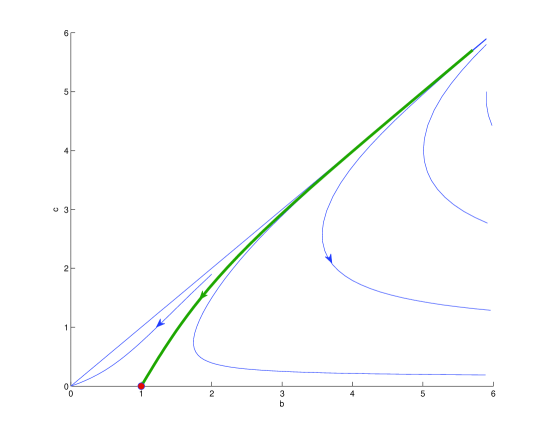
Figure 1. The flow line diagram of system (2.5)

3. The cross curvature flow on $\mbox{SL}(2,\mathbb{R})$

3.1. The ODE system

We now consider the cross curvature flow (1.2) where $g_{0}$ is a left-invariant metric on $\mbox{SL}(2,\mathbb{R})$. Let $g(t)$, $t\in(-T_{b},T_{f})$, be the maximal solution of the cross curvature flow through $g_{0}$. Writing

$$g=Af^{1}\otimes f^{1}+Bf^{2}\otimes f^{2}+Cf^{3}\otimes f^{3},$$

we obtain the system

(3.1) $$\left\{\begin{aligned} \frac{dA}{dt}=&-\frac{2AF_{2}F_{3}}{(ABC)^{2}},\\ \frac{dB}{dt}=&-\frac{2BF_{3}F_{1}}{(ABC)^{2}},\\ \frac{dC}{dt}=&-\frac{2CF_{1}F_{2}}{(ABC)^{2}},\end{aligned}\right.$$

where

$$F_{1}= -3A^{2}+B^{2}+C^{2}-2BC-2AC-2AB,$$

$$F_{2}= -3B^{2}+A^{2}+C^{2}+2BC+2AC-2AB,$$

$$F_{3}= -3C^{2}+A^{2}+B^{2}+2BC-2AC+2AB.$$

3.2. Asymptotic Results

Without loss of generality we assume throughout this section that $B_{0}\geq C_{0}$. Then $B\geq C$ as long as a solution exists. The behavior of the flow in the forward direction can be summarized as follows. See [CNSC08].

Theorem 3.1 ((XCF) Forward direction).

If $B_{0}=C_{0}$ then $T_{f}=\infty$ and there exists a constant $A_{\infty}\in(0,\infty)$ such that,

$$B(t)=C(t)\sim(24A_{\infty}t)^{1/3}\mbox{ and }A(t)\sim A_{\infty}\;\mbox{ as }t\rightarrow\infty.$$

If $B_{0}>C_{0}$, $T_{f}$ is finite and there exists a constant $E\in(0,\infty)$ such that,

$$A(t)\sim B(t)\sim E(T_{f}-t)^{-1/2}\mbox{ and }C(t)\sim 8(T_{f}-t)^{1/2}\;\mbox{ as }t\rightarrow T_{f}.$$

In the backward direction, the following was proved in [CSC08].

Theorem 3.2 ((XCF) Backward direction).

We have $T_{b}\in(0,\infty)$, i.e., the maximal backward existence time is finite. Moreover,

1. If there is a time $t<0$ such that $A(t)\geq B(t)-C(t)$ then, as $t$ tends to $-T_{b}$,

   $$A(t)\sim\eta_{1}(t+T_{b})^{-1/14},\;B(t)\sim\eta_{2}(t+T_{b})^{3/14},\;C(t)\sim\eta_{3}(t+T_{b})^{3/14}$$

   for some constants $\eta_{i}\in(0,\infty)$, $i=1,2,3$.

2. If there is a time $t<0$ such that $A<\frac{1}{3}\left(2\sqrt{B^{2}-BC+C^{2}}-B-C\right)$ then, as $t$ tends to $-T_{b}$,

   $$A(t)\sim\eta_{1}(t+T_{b})^{3/14},\;B(t)\sim\eta_{2}(t+T_{b})^{-1/14},\;C(t)\sim\eta_{3}(t+T_{b})^{3/14}$$

   for some constants $\eta_{i}\in(0,\infty)$, $i=1,2,3$.

3. If for all time $t<0$, $\frac{1}{3}\left(2\sqrt{B^{2}-BC+C^{2}}-B-C\right)\leq A<B-C$ then, as $t$ tends to $-T_{b}$,

   $$A(t)\sim 64\eta^{-1}(t+T_{b}),\;B(t)\sim\eta+4\sqrt{2(t+T_{b})},\;C(t)\sim\eta-4\sqrt{2(t+T_{b})}$$

   for some $\eta\in(0,\infty)$.

As far as the cross curvature flow is concerned, the goal of this paper is to show that the third case in the theorem above can only occur when the initial condition $(A_{0},B_{0},C_{0})$ belongs to a two dimensional hypersurface. In particular, it does not occur for a generic initial metric $g_{0}$ on $\mbox{SL}(2,\mathbb{R})$.

Theorem 3.3.

Let $Q=\{(a,b,c)\in\mathbb{R}^{3}:a>0,b>c>0\}$. There is an open dense subset $Q_{0}$ of $Q$ such that, for any maximal solution $g(t)$, $t\in(-T_{b},T_{f})$, of the cross curvature flow with initial condition $(A(0),B(0),C(0))\in Q_{0}$, as $t$ tends to $-T_{b}$,

1. either $A(t)\sim\eta_{1}(t+T_{b})^{-1/14},\;B(t)\sim\eta_{2}(t+T_{b})^{3/14},\;C(t)\sim\eta_{3}(t+T_{b})^{3/14}$

2. or $A(t)\sim\eta_{1}(t+T_{b})^{3/14},\;B(t)\sim\eta_{2}(t+T_{b})^{-1/14},\;C(t)\sim\eta_{3}(t+T_{b})^{3/14}$.

In fact, let $Q_{1}$ (resp. $Q_{2}$) be the set of initial conditions such case (1) (resp. case (2)) occurs. Then there exists a smooth embedded hypersurface $S_{0}\subset Q$ such that $Q_{1},Q_{2}$ are the two connected components of $Q\setminus S_{0}$. Moreover, for initial condition on $S_{0}$, the behavior is given by case (3) of Theorem 3.2.

In order to prove this result, it suffices to study case (3) of Theorem 3.2. In that case, it is proved in [CSC08] that $A$, $B$ and $C$ are monotone ($A,B$ non-decreasing, $C$ non-increasing) on $(-T_{b},0]$. In order to understand the behavior of the solution, and because of the homogeneous structure of the ODE system (3.1), we can pass to the affine coordinates $(A/C,B/C)$. This leads to a two-dimensional ODE system whose orbit structure can be analyzed.

Remark 3.1.

The analysis below shows that, in case (1) of Theorem 3.3 and when the initial condition varies, all the values larger than $1$ of the ratio $\eta_{2}/\eta_{3}$ are attained. Similarly, in case (2), all the values of the ratio $\eta_{1}/\eta_{3}$ are attained.

3.3. The two-dimensional ODE system for the cross curvature flow

For convenience, we introduce the backward cross curvature flow, for which the ODE is

(3.2) $$\left\{\begin{aligned} \frac{dA}{dt}=&\frac{2AF_{2}F_{3}}{(ABC)^{2}},\\ \frac{dB}{dt}=&\frac{2BF_{3}F_{1}}{(ABC)^{2}},\\ \frac{dC}{dt}=&\frac{2CF_{1}F_{2}}{(ABC)^{2}},\end{aligned}\right.$$

where $\{F_{i}\}_{1}^{3}$ are defined as before. By Theorem 3.2, the maximal forward solution of this system is defined on $[0,T_{b})$ with $T_{b}<\infty$.

Note that if $(A,B,C)$ is a solution, then

$$t\mapsto(\lambda A(t/\lambda^{2}),\lambda B(t/\lambda^{2}),\lambda C(t/\lambda^{2}))$$

is also a solution. By Theorem 3.2, there are solutions with initial values in $Q$ such that $A/B$ tends to $\infty$ and others such that $(A/B,C/B)$ tends to $(0,0)$. Let $Q_{1}$ be the set of initial values in $Q$ such that $A/B$ tends to $\infty$ and $Q_{2}$ be the set of those for which $(A/B,C/B)$ tends to $(0,0)$. Let $S_{0}$ be the complement of $Q_{1}\cup Q_{2}$ in $Q$. Again, by Theorem 3.2, for initial solution in $S_{0}$, $(A/B,C/B)$ tends to $(0,1)$.

The sets $Q_{1}$, $Q_{2}$, $S_{0}$ must be homogeneous cones, i.e., are preserved under dilations. Hence, they are determined by their projectivization on the plane $B=1$. So we set $a=A/B,\;\;c=C/B$ and compute

(3.3) $$\left\{\begin{array}[]{ccc}da/dt&=&\frac{8}{(Bac)^{2}}a(a+1)(a+c-1)\phi_{3}\\ dc/dt&=&-\frac{8}{(Bac)^{2}}c(1-c)(a+c+1)\phi_{1},\end{array}\right.$$

where

$$\phi_{1}= -3a^{2}+1+c^{2}-2c-2ac-2a,$$

$$\phi_{3}= -3c^{2}+a^{2}+1+2c-2ac+2a.$$

This means that, up to a monotone time change, the stereographic projection of any flow line of (3.2) on the plane $B=1$ is a flow line of the planar ODE system

(3.4) $$\left\{\begin{array}[]{ccc}da/dt&=&a(a+1)(a+c-1)\phi_{3}\\ dc/dt&=&-c(1-c)(a+c+1)\phi_{1}.\end{array}\right.$$

Set $\Omega=\{a>0,1>c>0\}$. By Theorem 3.2, any integral curve of (3.3) tends in the forward time direction to either $(0,0)$, $(\infty,c_{\infty})$, $0<c_{\infty}<\infty$, or $(0,1)$. The equilibrium points of (3.3), i.e., the points where $(da/dt,dc/dt)=(0,0)$, are $(0,0),(1,0),(0,1)$. To investigate the nature of these equilibrium points, we compute the Jacobian of the right-hand side of the ODE which is

$$\left(\begin{array}[]{cc}Y_{11}&Y_{12}\\ Y_{21}&Y_{22}\end{array}\right),$$

where

$$Y_{11} = (3a^{2}+2ac+c-1)\phi_{3}+2a(a+1)(a+c-1)(a-c+1),$$

$$Y_{12} = a(a+1)[\phi_{3}+2(a+c-1)(-3c+1-a)],$$

$$Y_{21} = -c(1-c)[\phi_{1}-2(a+c+1)(3a+c+1)],$$

$$Y_{22} = (3c^{2}+2ac-a-1)\phi_{1}-2c(1-c)(a+c+1)(c-1-a).$$

In particular, at $(0,0)$, this is $-1$ times the identity matrix and the equilibrium point $(0,0)$ is attractive. Its basin of attraction corresponds to region $Q_{2}$ defined above. At $(1,0)$, the Jacobian is $\left(\begin{array}[]{cc}8&8\\ 0&8\end{array}\right)$. This point is a repelling fixed point. It reflects the behavior of the forward Ricci flow described in Theorem 3.1($B>C$). At $(0,1)$, the Jacobian is $\left(\begin{array}[]{cc}0&0\\ 0&0\end{array}\right)$. This is the equilibrium point of interest to us and a more detailed analysis is required to determine trajectories that tend toward it. This is done with coordinate transformations that blow-up the equilibrium.

Blow-up transformations introduce coordinates in which the blown up equilibrium becomes a circle or projective line representing directions through the equilibrium. Blow-up transformations reduce the analysis of flows near degenerate equilibria to flows with less degenerate equilibria. The blown up system allows us to analyze the trajectories that are asymptotic to the equilibrium. In particular, trajectories approaching the equilibrium of the original system from different directions yield different equilibria in the blown up system.

Translating the equilibrium point to the origin by setting $e=c-1$, the equations (3.3) become

(3.5) $$\left\{\begin{array}[]{ccc}da/dt&=&-a(a+1)(a+e)(3e^{2}+4e+2ae-a^{2}),\\ de/dt&=&e(e+1)(a+e+2)(e^{2}-2ae-4a-3a^{2}).\end{array}\right.$$

The leading order terms of equations (3.5) have degrees 3 and 2: the next coordinate transformation $a=u^{2},e=v$ of the region $a\geq 0$ produces a system in which the leading terms of both equations have degree 3:

(3.6) $$\left\{\begin{array}[]{ccc}du/dt&=&-\frac{1}{2}u(u^{2}+1)(v+u^{2})(3v^{2}+4v+2u^{2}v-u^{4}),\\ dv/dt&=&v(v+1)(v+2+u^{2})(v^{2}-2u^{2}v-4u^{2}-3u^{4}).\end{array}\right.$$

To blow up the origin, the equations (3.6) are transformed to polar coordinates $(u,v)=(r\cos(\theta),r\sin(\theta))$ and then rescaled by a common factor of $r$, yielding the vector field $X$ defined by

(3.7) $$\left\{\begin{array}[]{ccl}dr/dt&=&1/2\,r[-33\,{r}^{3}\left(\cos\left(\theta\right)\right)^{4}\left(\sin\left(\theta\right)\right)^{3}-29\,{r}^{2}\left(\cos\left(\theta\right)\right)^{4}\left(\sin\left(\theta\right)\right)^{2}\\ &&-11\,{r}^{4}\left(\cos\left(\theta\right)\right)^{6}\left(\sin\left(\theta\right)\right)^{2}-{r}^{5}\left(\cos\left(\theta\right)\right)^{8}\sin\left(\theta\right)-5\,{r}^{3}\left(\cos\left(\theta\right)\right)^{6}\sin\left(\theta\right)\\ &&+{r}^{6}\left(\cos\left(\theta\right)\right)^{10}-35\,r\left(\cos\left(\theta\right)\right)^{2}\left(\sin\left(\theta\right)\right)^{3}-20\,\left(\cos\left(\theta\right)\right)^{2}\left(\sin\left(\theta\right)\right)^{2}\\ &&-4\,r\left(\cos\left(\theta\right)\right)^{4}\sin\left(\theta\right)+{r}^{4}\left(\cos\left(\theta\right)\right)^{8}+2\,{r}^{2}\left(\sin\left(\theta\right)\right)^{6}\\ &&-2\,{r}^{3}\left(\sin\left(\theta\right)\right)^{5}\left(\cos\left(\theta\right)\right)^{2}-18\,{r}^{2}\left(\cos\left(\theta\right)\right)^{2}\left(\sin\left(\theta\right)\right)^{4}\\ &&-10\,{r}^{4}\left(\sin\left(\theta\right)\right)^{4}\left(\cos\left(\theta\right)\right)^{4}+6\,r\left(\sin\left(\theta\right)\right)^{5}\\ &&-6\,{r}^{5}\left(\sin\left(\theta\right)\right)^{3}\left(\cos\left(\theta\right)\right)^{6}+4\,\left(\sin\left(\theta\right)\right)^{4}],\\ d\theta/dt&=&-1/2\,\cos\left(\theta\right)\sin\left(\theta\right)[-2\,{r}^{2}\left(\sin\left(\theta\right)\right)^{4}-{r}^{3}\left(\sin\left(\theta\right)\right)^{3}\left(\cos\left(\theta\right)\right)^{2}\\ &&+9\,{r}^{2}\left(\cos\left(\theta\right)\right)^{2}\left(\sin\left(\theta\right)\right)^{2}+5\,{r}^{4}\left(\sin\left(\theta\right)\right)^{2}\left(\cos\left(\theta\right)\right)^{4}-9\,r\left(\sin\left(\theta\right)\right)^{3}\\ &&+28\,r\left(\cos\left(\theta\right)\right)^{2}\sin\left(\theta\right)+25\,{r}^{3}\left(\cos\left(\theta\right)\right)^{4}\sin\left(\theta\right)+5\,{r}^{5}\sin\left(\theta\right)\left(\cos\left(\theta\right)\right)^{6}\\ &&-8\,\left(\sin\left(\theta\right)\right)^{2}+16\,\left(\cos\left(\theta\right)\right)^{2}+20\,{r}^{2}\left(\cos\left(\theta\right)\right)^{4}\\ &&+7\,{r}^{4}\left(\cos\left(\theta\right)\right)^{6}+{r}^{6}\left(\cos\left(\theta\right)\right)^{8}].\end{array}\right.$$

In these equations, the origin of equations (3.6) is blown up to the invariant circle $r=0$, and the complement of the origin becomes the cylinder $r>0$. Trajectories that tend to the origin in equation (3.6) yield trajectories that tend to an equilibrium point of equations (3.7) on the circle $r=0$. Now the zeros of $d\theta/dt$ on the circle $r=0$ are equilibria of the rescaled equations obtained from (3.7). They are located at points where $\cos^{2}(\theta)=0,1$ or $1/3$. The equilibria determine the directions in which trajectories of (3.6) can approach or leave the origin. These directions correspond to different approach to the equilibrium $(0,1)$ of (3.4). In the $(a,c)$ coordinates, the directions $\theta=\pm\pi/2$ correspond to approaching $(0,1)$ along curves tangent to the $c$-axis with tangency degree greater than $2$. The direction $\theta=0$ corresponds to approaching $(0,1)$ along curves tangent to $c=1$. The directions $\pm\theta_{0}$ with $\cos^{2}\theta_{0}=1/3$ correspond to approaching $(0,1)$ along curves asymptotic to the parabola $a=\frac{1}{2}(c-1)^{2}$. Observe that this is consistent with Theorem 3.2(3). Our goal is to show that this can only happen along a particular curve.

Since the circle $r=0$ is invariant, the Jacobians at the equilibria discussed above are triangular. The stability of each equilibrium is determined by the signs of $\frac{1}{r}(dr/dt)$ and $\partial(d\theta/dt)/\partial\theta$ when these are non-zero. The equilibria with $\cos^{2}(\theta)=0$ have $\frac{1}{r}(dr/dt)=2$ and $\partial(d\theta/dt)/\partial\theta=-4$, so the point is a saddle with an unstable manifold in the region $r>0$. Equilibria with $\cos^{2}(\theta)=1/3$ have $\frac{1}{r}(dr/dt)=-4/3$ and $\partial(d\theta/dt)/\partial\theta=16/3$, so these equilibria are also saddles but with stable manifolds in the region $r>0$. After change of coordinates, only one of these stable manifolds, call it $\gamma_{0}$, belongs to the region $\{c<1\}$. This curve $\gamma_{0}$ provides the only way to approach $(0,1)$ which is consistent with case (3) of Theorem 3.2. The equilibria with $\cos^{2}(\theta)=1$ have $\frac{1}{r}(dr/dt)=0$ and $\partial(d\theta/dt)/\partial\theta=-8$, so further analysis is required to determine the properties of nearby trajectories. However, because of Theorem 3.2, it is clear that any solution of (3.4) approaching the line $\{c=1\}$ has $a\rightarrow\infty$, hence cannot approach $(1,0)$. The following argument recovers this fact directly from (3.7).

Note that when $\theta=0$, $d\theta/dt=0$ and $dr/dt=(r^{5}+r^{7})/2$. Therefore, the $r$ axis is invariant and weakly unstable. The trajectory along this axis approaches $(0,0)$ as $t\to-\infty$. To prove that no other trajectories in $r>0$ approach the origin as $t\to\pm\infty$, we consider the vector field $Y$ defined by subtracting $r^{5}\cos^{8}(\theta)/2+r^{7}\cos^{10}(\theta)/2$ from $dr/dt$ in $X$:

(3.8) $$\left\{\begin{array}[]{ccl}dr/dt&=&1/2\,\sin\left(\theta\right)r[-5\,{r}^{3}\left(\cos\left(\theta\right)\right)^{6}-4\,r\left(\cos\left(\theta\right)\right)^{4}\\ &&-29\,{r}^{2}\left(\cos\left(\theta\right)\right)^{4}\sin\left(\theta\right)-20\,\sin\left(\theta\right)\left(\cos\left(\theta\right)\right)^{2}-35\,r\left(\cos\left(\theta\right)\right)^{2}\left(\sin\left(\theta\right)\right)^{2}\\ &&-{r}^{5}\left(\cos\left(\theta\right)\right)^{8}-11\,{r}^{4}\left(\cos\left(\theta\right)\right)^{6}\sin\left(\theta\right)-33\,{r}^{3}\left(\cos\left(\theta\right)\right)^{4}\left(\sin\left(\theta\right)\right)^{2}\\ &&-6\,{r}^{5}\left(\cos\left(\theta\right)\right)^{6}\left(\sin\left(\theta\right)\right)^{2}-10\,{r}^{4}\left(\cos\left(\theta\right)\right)^{4}\left(\sin\left(\theta\right)\right)^{3}\\ &&-2\,{r}^{3}\left(\cos\left(\theta\right)\right)^{2}\left(\sin\left(\theta\right)\right)^{4}-18\,{r}^{2}\left(\cos\left(\theta\right)\right)^{2}\left(\sin\left(\theta\right)\right)^{3}+6\,r\left(\sin\left(\theta\right)\right)^{4}\\ &&+2\,{r}^{2}\left(\sin\left(\theta\right)\right)^{5}+4\,\left(\sin\left(\theta\right)\right)^{3}],\\ d\theta/dt&=&-1/2\,\cos\left(\theta\right)\sin\left(\theta\right)[-2\,{r}^{2}\left(\sin\left(\theta\right)\right)^{4}-{r}^{3}\left(\sin\left(\theta\right)\right)^{3}\left(\cos\left(\theta\right)\right)^{2}\\ &&+9\,{r}^{2}\left(\cos\left(\theta\right)\right)^{2}\left(\sin\left(\theta\right)\right)^{2}+5\,{r}^{4}\left(\sin\left(\theta\right)\right)^{2}\left(\cos\left(\theta\right)\right)^{4}-9\,r\left(\sin\left(\theta\right)\right)^{3}\\ &&+28\,r\left(\cos\left(\theta\right)\right)^{2}\sin\left(\theta\right)+25\,{r}^{3}\left(\cos\left(\theta\right)\right)^{4}\sin\left(\theta\right)\\ &&+5\,{r}^{5}\sin\left(\theta\right)\left(\cos\left(\theta\right)\right)^{6}-8\,\left(\sin\left(\theta\right)\right)^{2}+16\,\left(\cos\left(\theta\right)\right)^{2}+20\,{r}^{2}\left(\cos\left(\theta\right)\right)^{4}\\ &&+7\,{r}^{4}\left(\cos\left(\theta\right)\right)^{6}+{r}^{6}\left(\cos\left(\theta\right)\right)^{8}].\par\end{array}\right.$$

The vector field $Y$ is transverse to the vector field $X$ in the interior of the first quadrant: $d\theta/dt<0$ for both $X$ and $Y$ and the $r$ component of $X$ is larger than the $r$ component of $Y$. Therefore, trajectories of $X$ cross the trajectories of $Y$ from below to above as they move left in the $(\theta,r)$ plane. The vector field $Y$ has a common factor of $\sin(\theta)$ in its two equations. When $Y$ is rescaled by dividing by this factor, the result is a vector field that does not vanish in a neighborhood of the origin. Since the $\theta$ axis is invariant for $Y$, the $Y$ trajectory $\gamma$ starting at $(\theta,r),\,r>0$ approaches the $r$ axis at a point with $r>0$. The $X$ trajectory starting at $(\theta,r)$ lies above $\gamma$, so it does not approach the origin. This proves that the only trajectories of equations (3.7) asymptotic to the origin lie on the $r$ and $\theta$ axes.

In conclusion, the above analysis shows that the regions $Q_{1}$, $Q_{2}$ are separated by the $2$-dimensional cone $S_{0}$ determined by the curve $\gamma_{0}$ in the $(a,c)$-plane. This proves Theorem 3.3. Figure 2 describes the flow lines of (3.4). The part of interest to us is the part below the line $\{c=1\}$, which corresponds to $\{B>C\}$. The part above the line $\{c=1\}$ corresponds to the case $\{B<C\}$, where the role of $B$ and $C$ are exchanged. The most important component of this diagram are the flow lines that are forward asymptotic to $(0,1)$. They correspond to the hypersurface $S_{0}$ in Theorem (3.3). The flow lines in the upper-left corner have vertical asymptotes $\{a=a_{\infty}\}$ with all positive values of $a_{\infty}$ appearing. Similarly, the flow lines on the right have horizontal asymptotes $\{c=c_{\infty}\}$ with all positive values of $c_{\infty}$ appearing. These facts can easily be derived from the system (3.4). This proves the part of Remark 3.1 dealing with case (1) of Theorem 3.3. The other case is similar using different coordinates.

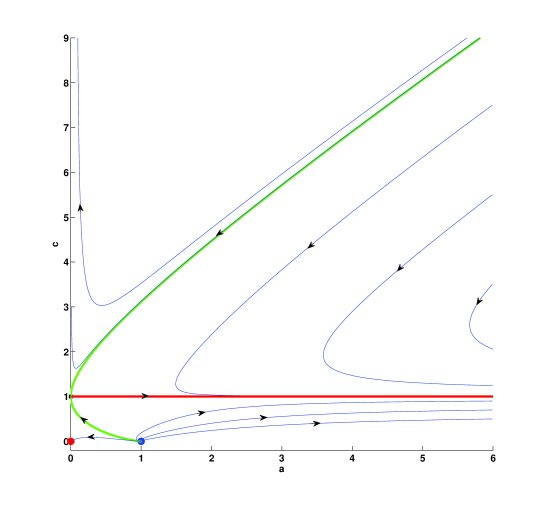
Figure 2. The flow line diagram of system (3.4)

References

- [CH04] Bennett Chow and Richard S. Hamilton. The cross curvature flow of 3-manifolds with negative sectional curvature. Turkish J. Math., 28(1):1–10, 2004.
- [CNSC08] Xiaodong Cao, Yilong Ni, and Laurent Saloff-Coste. Cross curvature flow on locally homogeneous three-manifolds. I. Pacific J. Math., 236(2):263–281, 2008.
- [CSC08] Xiaodong Cao and Laurent Saloff-Coste. The cross curvature flow on locally homogeneous three-manifolds (II). Asian J. Math., to appear, 2008, http://arxiv.org/abs/0805.3380.
- [CSC09] Xiaodong Cao and Laurent Saloff-Coste. Backward Ricci flow on locally homogeneous 3-manifolds. Comm. Anal. Geom., 17(2):305–325, 2009.
- [Gli08] David Glickenstein. Riemannian groupoids and solitons for three-dimensional homogeneous Ricci and cross-curvature flows. Int. Math. Res. Not. IMRN, (12):Art. ID rnn034, 49, 2008.
- [Ham82] Richard S. Hamilton. Three-manifolds with positive Ricci curvature. J. Differential Geom., 17(2):255–306, 1982.
- [IJ92] James Isenberg and Martin Jackson. Ricci flow of locally homogeneous geometries on closed manifolds. J. Differential Geom., 35(3):723–741, 1992.
- [KM01] Dan Knopf and Kevin McLeod. Quasi-convergence of model geometries under the Ricci flow. Comm. Anal. Geom., 9(4):879–919, 2001.
- [Lot07] John Lott. On the long-time behavior of type-III Ricci flow solutions. Math. Ann., 339(3):627–666, 2007.
- [Mil76] John Milnor. Curvatures of left invariant metrics on Lie groups. Advances in Math., 21(3):293–329, 1976.
- [Mon02] Richard Montgomery. A tour of subriemannian geometries, their geodesics and applications, volume 91 of Mathematical Surveys and Monographs. American Mathematical Society, Providence, RI, 2002.
- [Sin60] I. M. Singer. Infinitesimally homogeneous spaces. Comm. Pure Appl. Math., 13:685–697, 1960.