Constraining dust and color variations of high-z SNe using NICMOS on the Hubble Space Telescope111Based on observations made with the NASA/ESA Hubble Space Telescope, obtained from the data archive at the Space Telescope Institute. STScI is operated by the association of Universities for Research in Astronomy, Inc. under the NASA contract NAS 5-26555. The observations are associated with program GO-07850.
Abstract
We present data from the Supernova Cosmology Project for five high redshift Type Ia supernovae (SNe Ia) that were obtained using the NICMOS infrared camera on the Hubble Space Telescope. We add two SNe from this sample to a rest-frame -band Hubble diagram, doubling the number of high redshift supernovae on this diagram. This -band Hubble diagram is consistent with a flat universe ( ) = (0.29, 0.71). A homogeneous distribution of large grain dust in the intergalactic medium (replenishing dust) is incompatible with the data and is excluded at the 5 confidence level, if the SN host galaxy reddening is corrected assuming . We use both optical and infrared observations to compare photometric properties of distant SNe Ia with those of nearby objects. We find generally good agreement with the expected color evolution for all SNe except the highest redshift SN in our sample (SN 1997ek at ) which shows a peculiar color behavior. We also present spectra obtained from ground based telescopes for type identification and determination of redshift.
1 Introduction
A decade ago, the development of Type Ia supernova (SNe Ia) as distance indicators began making possible precise measurements of the expansion history, leading to the understanding that a dark energy dominates the fate of our Universe (Perlmutter et al., 1998; Garnavich et al., 1998; Schmidt et al., 1998; Riess et al., 1998; Perlmutter et al., 1999). With the advent of increasingly larger and more precise SNe Ia surveys, which aim to elucidate the nature of dark energy, it has become clear that systematic uncertainties are a limiting factor (Knop et al., 2003; Tonry et al., 2003; Astier et al., 2006; Wood-Vasey et al., 2007b; Riess et al., 2007; Kowalski et al., 2008). In particular, knowledge of SNe intrinsic colors and dimming due to extinction by dust in the host galaxy have been identified as the dominant systematic effects for the determination of cosmological parameters, see e.g., Nordin et al. (2008). It is often assumed that dust in distant galaxies resembles the dust in the Milky Way, whose properties are well studied and for which maps of dust distribution and composition are available. This question, however, remains unresolved. Another source of uncertainty is in our knowledge of the SN intrinsic color and its dispersion, which is normally used for determining the amount of reddening222One normally refers to reddening as an effect of dust extinction, either in the SN host galaxy or in the Milky-Way. However, there could be a relation between colors and intrinsic brightness of SNe Ia that mimics an extinction law, though not caused by differential dimming by dust. Thus, we use the term color excess to describe the deviation from the average color, irrespective of the underlying mechanism causing the offset. for each supernova. Moreover, the understanding of the mechanisms leading to the explosion of SNe Ia or the nature of the progenitor systems is still incomplete. Thus, the empirical properties of the standard candles need to be continuously compared between distant and nearby objects. While there is evidence for evolution in average SN properties with redshift (Howell et al., 2007), no intrinsic SN evolution has been observed in the spectral and photometric properties of individual objects (see e.g., Nobili et al. (2005); Blondin et al. (2006); Garavini et al. (2007); Ellis et al. (2008); Foley et al. (2008); Bronder et al. (2008); Riess et al. (2007)).
Dust extinction has a strong wavelength dependence. Milky-Way type dust causes twice as much extinction in the -band as in the -band, and a factor of 4 more in the -band than in the -band. This suggests that observations in the near-infrared and infrared () are a very powerful tool for minimizing systematic uncertainties in supernova cosmology due to the determination of the host galaxy extinction (Nobili et al., 2005; Wood-Vasey et al., 2008a). However, ground-based infrared observations require relatively long exposures and are limited by atmospheric emission and absorption. Observations from space have significantly better resolution and less background contamination leading to more precise infrared photometry from space than from the ground.
In this paper, we use Near-Infrared Camera and Multi-Object Spectrometer (NICMOS) infrared and Wide Field Planetary Camera 2 (WFPC2) optical data to study the colors of five distant SNe Ia over a broad range of rest-frame wavelengths. In Section 2, we present the photometric data. In Section 3, we show the spectra collected for the type identification and determination of redshift. We compare the observed optical and infrared colors with those of nearby SNe Ia in Section 4. In Section 5, we add two SNe from our sample to the current rest-frame -band Hubble diagram, doubling the number of SNe and extending the analysis to . Finally, we discuss our results in Section 6.
2 The data set
We present data of 5 distant Type Ia supernovae that were obtained with the NICMOS mounted on the Hubble Space Telescope (HST). These supernovae, in the redshift range , were discovered by the Supernova Cosmology Project during ground based searches for SNe Ia conducted with the 4m Blanco telescope at the Cerro Tololo Inter-American Observatory (CTIO) in 1997 and 1998. Optical follow up observations were carried out from the ground and from space and have been presented in previous work (Knop et al., 2003). These consist of multi-epoch observations with the WFPC2 camera on HST in the and broadband filters and multi-epoch ground-based observations in the and bands. The HST filter pair and the ground-based filter pair both correspond to rest-frame and for and to rest-frame and for .
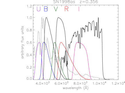
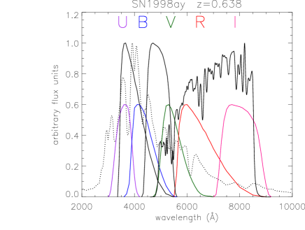
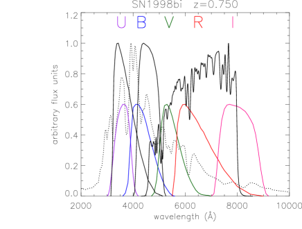
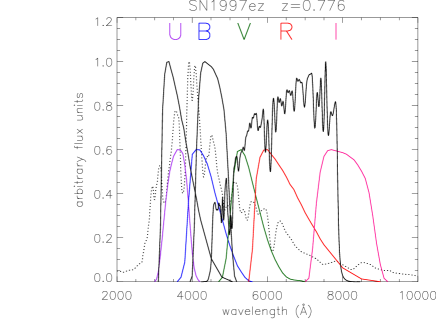
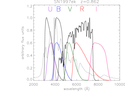
Infrared images were obtained using the broadband filter on the NIC2 camera. Given the broad redshift range of the SNe, the filter corresponds to different rest-frame filters as shown in Figure 1.
Some of the NICMOS data were affected by the passage of HST through the South Atlantic Anomaly prior to the observations. After visual examination, good images were processed with a modified version of the STScI pipeline. Details of the modifications are explained in Fadeyev et al. (2006) and include an improved technique for evaluating per-pixel count rate errors and a different method for correcting the cosmic ray (CR) hits. Although the standard STScI pipeline also evaluates the count rate errors, the modifications improved the statistical correspondence between the errors and fluctuations in the sky level and were used to estimate the photometric errors. The standard bias equalization procedure was used during the processing. The images were corrected for the rate dependent non-linearity effect (Bohlin et al., 2005; de Jong, 2006).
PSF photometry was done on the processed images with TinyTIM models (Krist & Hook, 2004). We have used standard star observations to verify that PSF photometry with TinyTIM is consistent with simple aperture photometry to 1% accuracy. The procedure was similar to the chi-square fitter used for optical photometry in Knop et al. (2003). There were two main differences due to features of the infrared data, as compared to the CCD-based observations. (1) The pixel flux uncertainty was taken from the modified pipeline evaluation. (2) Bad pixels, a frequent occurrence in NICMOS arrays, were explicitly omitted from the chi-square evaluation.
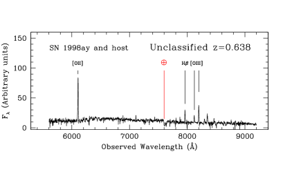
For most SNe, the distance to the host galaxy was sufficiently large that the host galaxy light could be modeled by a second degree polynomial. In these cases, the reference images were used to visually examine the SN location for unusual host galaxy shapes. The only exception was SN 1998ay, where an elliptical-like galaxy model was used in a joint fit with the final reference images. We have evaluated the systematic uncertainties due to host galaxy modeling and CR rejection to be typically at the 1–4% level, although there were a couple of cases as large as 10–18%.
Because the NICMOS detectors have a count-rate dependent non-linearity we correct for (often referred to as the Bohlin Effect (Shaw & de Jong, 2008)), we must apply a corresponding zeropoint, , to derive Vega magnitudes. Our data were acquired when the NICMOS IR arrays were operating at a temperature of 60 K. For this temperature, STScI only provides zero points for standard calibrations. The well modeled detector non-linearity corrections are based on an operating temperature of 77 K. We assume that the non-linear corrections at 60 K are the same as at 77 K333This is supported by the fact that the NICMOS array response only changed by about 50% after installation of the cryocooler. On the scale of the non-linearity correction, 0.05 mag per decade of flux change, the effect of extra 50% flux nominally results in 0.009 mag correction, a negligible amount., namely, . We obtain = 22.268.
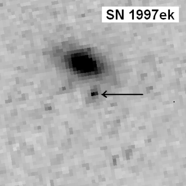
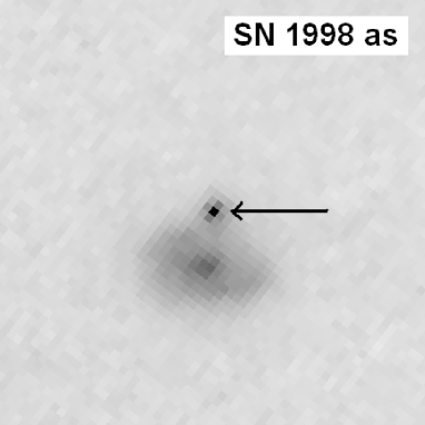
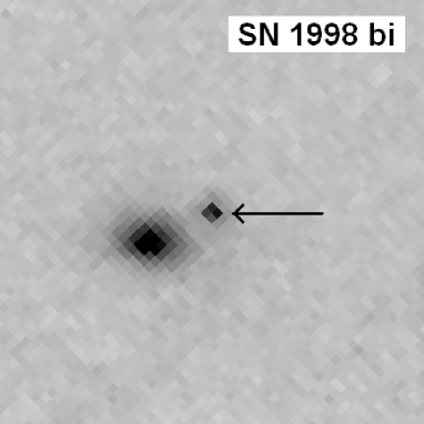
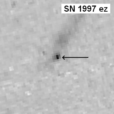
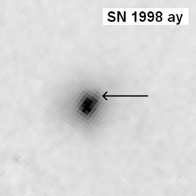
A summary of the observations is given in Table 1, including the time since -band maximum, exposure time in seconds, magnitudes in the Vega system, and total uncertainties (including both statistical and systematic). Figure 2 shows the infrared image taken at the brightest epoch observed. Each image, covering 4 4 arcsecs, is built by co-adding several observations for the purpose of displaying the position of the SN with respect to the host galaxy. The actual photometry was performed on the individual images. Table 2 reports redshifts, -band stretch factors, Milky Way reddenings, and color excesses for these SNe.
| SN | MJD | EpochaaDays since B-band maximum in the observer frame. | ExpbbExposure time in seconds. | CountsccCounts (ADUs) per second. For conversion to electrons per second one can use the gain of 5.4 e-/ADU Barker & Dahlen (2007). The first uncertainty shown is statistical and the second one is systematic. | Vega magnitudesddInfrared Photometry. The uncertainty includes both statistical and systematic components, as well as a 2% zeropoint calibration uncertainty. |
|---|---|---|---|---|---|
| SN 1997ek | 50818.50 | -0.07 | 1026 | 0.483 0.055 0.014 | 23.058 0.126 |
| 50824.34 | 5.77 | 2053 | 0.508 0.020 0.017 | 23.003 0.055 | |
| 50846.73 | 28.16 | 1280 | 0.441 0.033 0.049 | 23.157 0.144 | |
| 50858.69 | 40.12 | 2560 | 0.253 0.017 0.017 | 23.760 0.101 | |
| 50872.10 | 53.53 | 2560 | 0.171 0.021 0.030 | 24.186 0.232 | |
| SN 1997ez | 50818.64 | 5.34 | 2052 | 0.466 0.018 0.011 | 23.097 0.050 |
| 50824.55 | 11.25 | 2052 | 0.523 0.019 0.011 | 22.972 0.047 | |
| 50858.63 | 45.33 | 2560 | 0.231 0.017 0.007 | 23.859 0.087 | |
| 50872.27 | 58.97 | 2560 | 0.232 0.018 0.010 | 23.854 0.096 | |
| SN 1998bi | 50922.51 | 10.70 | 3593 | 0.607 0.014 0.015 | 22.810 0.037 |
| SN 1998as | 50909.35 | 13.23 | 5134 | 0.882 0.013 0.026 | 22.404 0.036 |
| 50921.27 | 25.15 | 5134 | 0.879 0.013 0.026 | 22.408 0.037 | |
| SN 1998ay | 50910.33 | 14.15 | 4105 | 0.554 0.017 0.012 | 22.909 0.040 |
| 50920.28 | 24.10 | 4105 | 0.409 0.015 0.009 | 23.239 0.047 |
| SN | ||||
|---|---|---|---|---|
| SN 1997ekbbThe color excess for SN 1997ek is estimated excluding the data point at day . See text for details. | 0.862 | 1.059 0.071 | 0.042 | |
| SN 1997ez | 0.776 | 1.094 0.038 | 0.026 | |
| SN 1998as | 0.356 | 0.931 0.018 | 0.037 | |
| SN 1998ay | 0.638 | 1.050 0.045 | 0.035 | |
| SN 1998bi | 0.75 | 0.975 0.031 | 0.026 |
3 Spectroscopic confirmation
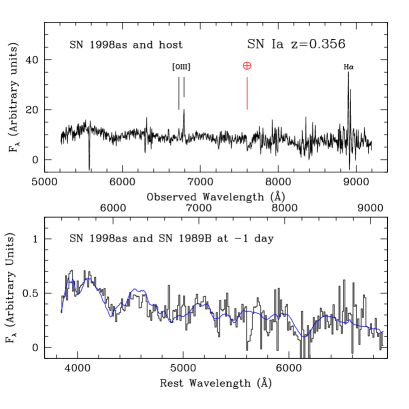
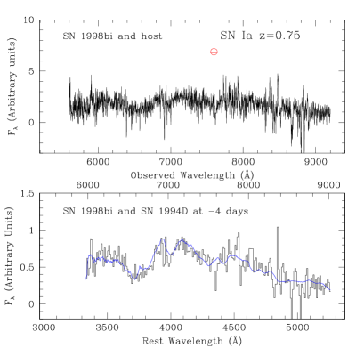
Optical spectra of SN 1997ek, SN 1997ez, SN 1998ay, and SN 1998bi were obtained at Mauna Kea (Keck II telescope) in December 1997 and April 1998. A spectrum of SN 1998as was obtained at the European Southern Observatory 3.6-m telescope in March 1998. All supernovae were within 2.5 arcsecs of the host galaxy center. Since Knop et al. (2003), the spectra have been re-analysed and the redshifts re-determined. In general, redshifts are measured from host galaxy emission and absorption lines. The one exception is SN 1998bi, for which the supernova was used. Within the uncertainties, the redshifts agree with those in Knop et al. (2003).
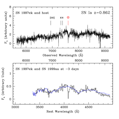
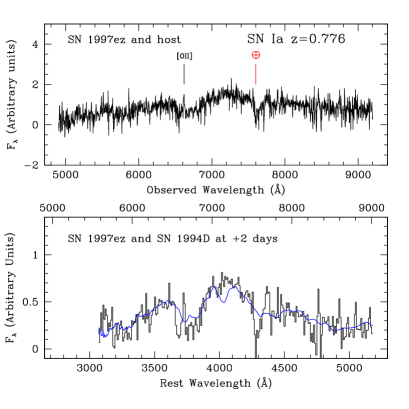
The extracted spectra, which consist of light from both the supernova and the host galaxy, were fitted with the algorithm described in Howell et al. (2005). The type, the confidence that the supernova is a SN Ia, and the mean rest-frame spectral age from the five best fits are shown in Table 3. The extracted spectra, the host-subtracted spectra, and the best matching local SN Ia are shown in Figure 3. With the exception of SN 1998ay, all of the SNe could be identified as either a certain SN Ia (confidence index of 5) or a highly probable one (confidence index of 4) . The spectrum of SN 1998ay is heavily contaminated with host galaxy light so a secure classification based on the spectrum is not possible. However, as we show in the next section, the light curve and color of SN 1998ay are consistent with those of a SN Ia.
| SN | Telescope | Instrument/SetupaaFor the LRIS observations, 400/8500/1 means that the observations were done with the 400/8500 grating and the 1″ slit. For the EFOSC II observations, R300/1.5 means that the observations were done with the R300 grism and the 15 slit. | Date(UT) | ExposurebbExposure time expressed in seconds | Best Match | Host Lines | EpochccAverage rest-frame epoch of the five best fits, with the rms value reported in parenthesis | Index | Classification |
|---|---|---|---|---|---|---|---|---|---|
| SN 1997ek | Keck II | LRIS/400/8500/1 | 02/01/1998 | 3x1500 | SN 1999aa -3 days | [O II],H,K | -1.8 (4.1) | 4 | SN Ia |
| SN 1997ez | Keck II | LRIS/300/5000/1 | 31/12/1997 | 3x1800 | SN 1994D +2 days | [O II] | +0.4 (6.4) | 4 | SN Ia |
| SN 1998as | ESO 3.6m | EFOSCII/R300/1.5 | 28/03/1998 | 2x1800 | SN 1989B -1 day | H, [O III], H | -1.8 (4.3) | 5 | SN Ia |
| SN 1998ay | Keck II | LRIS/400/8500/1 | 03/04/1998 | 2x1200 | No match | [O II], H, [O III] | 2 | SN | |
| SN 1998bi | Keck II | LRIS/400/8500/1 | 01/04/1998 | 1x1500 | SN 1994D -4 days | -3.4 (3.9) | 5 | SN Ia |
4 Supernova colors
We use the infrared data together with the optical data presented by Knop et al. (2003) to compare photometric properties of distant SNe Ia to those of nearby SNe Ia. Intrinsic color properties of nearby SNe Ia have been extensively studied by Nobili & Goobar (2008). The reported color evolution with stretch and supernova epoch are used in the analysis presented here, both as a model for the intrinsic colors and for the -corrections (Kim et al., 1996). Nugent et al. (2002) showed that the latter depends mainly on the supernova color rather than on changes in individual spectral features. Thus we use the spectral templates developed by Hsiao et al. (2007) modified by the color-stretch relation determined in Nobili & Goobar (2008) before computing the -corrections. To compare the observed colors of the SNe in this data-set with color templates derived for low-z supernovae we need to know three parameters: the epochs of our observations with respect to restframe -band maximum, the stretch of the rest-frame -band lightcurve and the color excess, . To obtain these parameters, the lightcurves need to be fitted iteratively, since the -corrections needed for the fits depend on both and . We use the following procedure:
-
1.
Compute -corrections using the spectral template corrected for the color excess, i.e. warped by the extinction law by Cardelli et al. (1989) (CCM) with the values of for each SN from Knop et al. (2003) using a total to selective extinction ratio , which has been found to give a good empirical description of reddening in low-z SNIa samples (Nobili & Goobar, 2008, and references therein).
-
2.
Fit the optical light curves to determine the time of -band maximum and the stretch factor, , for each SN.
-
3.
Compute the intrinsic colors corresponding to following the color-stretch relation described in Nobili & Goobar (2008)
-
4.
Warp the spectral templates444We use a cubic spline interpolation of the ratio between the synthetic photometry and the new photometry at the effective wavelengths. The -band light curve by Goldhaber et al. (2001) is assumed in order to compute all the bands given the colors , , and (see Nobili & Goobar (2008) for details). to match the expected colors for the fitted . We also redden the spectral template assuming as a first approximation the color excess determined by Knop et al. (2003). Thus, we use the modified spectral template to compute -corrections, while keeping the measured colors unchanged.
-
5.
Fit the optical light curves again using updated K-corrections
-
6.
Build the color models using the fitted -band light curve model interpolated to the epochs of the -band observations to compute , and to the epochs of the -band observations to compute .
Note that, in the previous steps we have not corrected the observed photometry for the extinction in the Milky Way or in the host galaxy. Instead, we have modified the spectral template needed for fitting the data. We use a grid of values of in steps of 0.01 mag with a spectral template reddened according to the CCM extinction law. We assume a value of the parameter as in Nobili & Goobar (2008). We note that a recent work by Goobar (2008) provides a potential explanation for the empirically found low average value of the total to selective extinction ratio in Type Ia supernovae as being a result of interaction with dust in the circumstellar environment, (see also Wang (2005)). Step 4 above is repeated until the fit parameters do not change outside the estimated uncertainties.
Finally, we compute synthetic photometry and build model color curves in the observer-frame filters, and , for each SN, reddened by the Milky Way extinction (Schlegel et al., 1998), using the standard value . The estimated color excess, , giving the best fit to the observed optical data, , is reported in Table 2. These values are then used to redden the color curves before comparing with the observed infrared data.
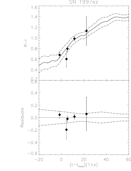
Figures 4- 6 show the comparison between the color curves obtained by synthetic photometry and the observed data. The filled symbols show the observed colors, whereas the color curves (solid lines) are the expected color evolution. The dashed lines represent the intrinsic dispersion for the given color, determined using the results in Nobili & Goobar (2008). Table 2 summarizes the results of this procedure. We note that the values of the stretch and color excess are slightly different from those reported in Knop et al. (2003). The discrepancies depend mainly on the different intrinsic colors assumed, in particular in , and on the spectral template and color-stretch relation used. Since the models assumed here are based on a larger sample, small discrepancies are not surprising (see also the discussion in Nobili & Goobar (2008)). We note that most of the differences are within one standard deviation from the quoted uncertainties.
We measured a large color excess, , for the lowest redshift SN in our sample (SN 1998as at ). As shown in Figure 1, the F110W filter at this redshift covers rest-frame , , and extends to about 11000 Å effectively covering rest-frame -band. Thus, the infrared data explore the red region of this SN spectrum which is less affected by reddening. These data offer the possibility to explore intrinsic color properties of SNe Ia despite the large color excess in the blue bands. Since the analysis presented by (Nobili & Goobar, 2008) extends only to the -band, the colors of the spectral template beyond this band are obtained by extrapolation to longer wavelengths. However, the spectral templates are quite featureless at these wavelengths and we expect very smooth behavior from the -band to the -band. This gives us confidence about the average color evolution within the assumed intrinsic dispersion. We note that the data agree with the expected color curves.
SN 1997ek shows an interesting color behavior. Its optical color is slightly bluer than expected and consistent with no extinction, but its infrared colors are substantially redder than average, as shown in Figure 6. We note that mis-measurement of the SN flux due to host galaxy contamination can be excluded due to the smooth profile and low flux level seen in the reference image of the galaxy. Moreover, the time evolution does not follow the behavior expected around 20 days after maximum brightness, as shown in the left panel of Figure 6. For this reason the color excess has been estimated using only the filled symbols in the figure. Given the different behaviors shown by this SN, we have compared its colors with those of the very peculiar nearby SN 2000cx (Li et al., 2001a; Candia et al., 2003; Branch et al., 2004). Pre-maximum spectra of SN 2000cx resemble that of the over-luminous SN 1991T and its color evolution is quite different from that of a normal Type Ia. The fact that the pre-maximum spectrum of SN 1997ek is well fitted by spectroscopically SN 1991T-like SN 1999aa, together with its peculiar colors, has prompted us to attempt a comparison of these two SNe. We have warped the spectral template with photometry of SN 2000cx before computing synthetic photometry with the passband filters used for the observations of SN 1997ek. The resulting color curves are shown as dotted lines in Figure 6. The agreement is improved in the infrared around maximum, but not at later times where SN 2000cx has colors similar to those of a normal SN Ia. Moreover, the dotted curve does not fit the observed data in the optical. We note that, if only the optical data at maximum were available, one would conclude that this SN is quite normal. The peculiar color behavior of SN 1997ek could be an indication of an intrinsic peculiarity of this SN. We note that the confidence index for the spectral typing of SN 1997ek is 4. Although it is not as secure as candidate that has clear SNe Ia features, such as Si II or S II, it is unlikely to be a SN of a different type.
The value of determined from the optical data gives a good agreement between the model and observed infrared color, giving a value of the for all cases except SN 1997ek. We take the good agreement found in the case of SN 1998ay as a confirmation that this is indeed a Type Ia SN.
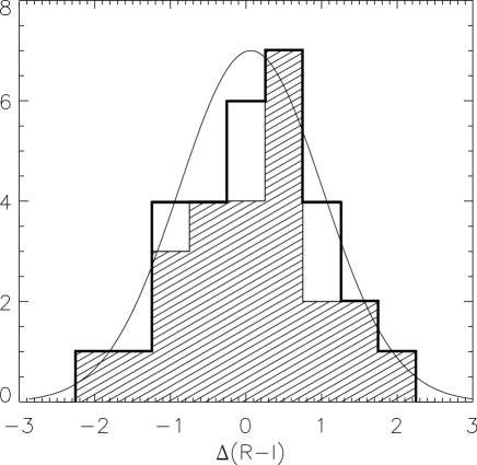
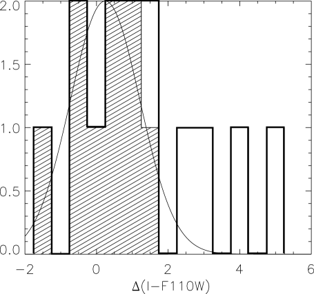
We compare the total distribution of the residuals of our sample with the expected distribution of nearby SNe. We normalize the residual of each data point from the expected color by dividing by the total uncertainty. The total uncertainty is calculated as a quadratic sum of the measurement uncertainty and the intrinsic dispersion:
Figure 7 shows the pull distribution for all SNe in each observed color. The shaded area include all SNe except the peculiar SN 1997ek. This is consistent with a Gaussian distribution, with zero mean and . Since the intrinsic dispersion used is based on measurements of nearby SNe, we can conclude that the same average color dispersion is observed in the distant sample.


4.1 SN 1999ff and SN 2000fr
Nobili et al. (2005) presented ground-based infrared observations for one SN Ia, SN 2000fr at redshift . This SN together with SN 1999ff at (Tonry et al., 2003) was compared to nearby SNe Ia and used to build a rest-frame -band Hubble diagram. We present the result of a re-analysis of these data, using the same technique applied to our 5 SNe in the previous section. Figure 8 shows optical and infrared color evolutions for both SNe. Table 4 summarizes the results.


| SNaaFrom Nobili et al. (2005) | ||||
|---|---|---|---|---|
| SN 1999ff | 0.455 | 0.82 0.05 | 0.025 | |
| SN 2000fr | 0.543 | 1.054 0.012 | 0.030 |
We note that the color excess giving the best fit to the optical data is consistent with no reddening for both SNe. The infrared data also agree with the expected behavior within the uncertainties.
5 -band Hubble diagram
Two SNe in our sample are at a redshift where the infrared observations correspond to the rest-frame -band (see Figure 1). These are SN 1998as () and SN 1998ay (). We note that SN 1998as has the largest extinction in our sample and SN 1998ay does not have a confirming spectrum, but is fully consistent with a SN Ia due to its colors and light curve shapes. We used these SNe to extend the -band Hubble diagram built by (Nobili et al., 2005) which originally included 2 SNe: SN 2000fr at and SN 1999ff at .
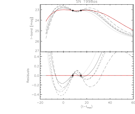
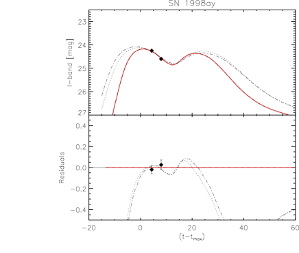
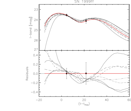
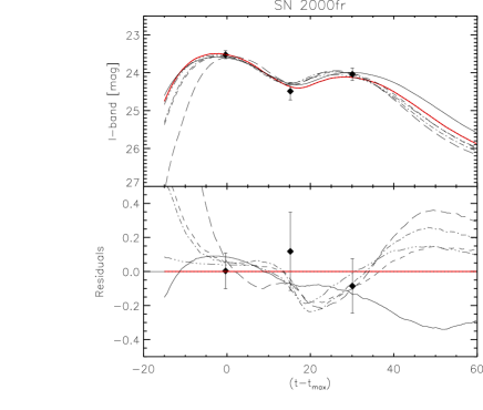
We computed -corrections for all four SNe from the observed infrared filter to rest-frame -band following Nobili & Goobar (2008). Using the -band templates of 42 nearby SNe Ia developed in Nobili et al. (2005) we fit the peak brightness of the high-redshift SNe. Figure 9 shows the template fits that satisfied , where is the of the best fitting template. The fitted giving the minimum is reported in Table 5. However, since several templates correspond to a similar value of the , we estimated the uncertainty, , as the rms of the peak magnitudes that satisfied .
Note that, given the different way of computing -corrections, the results obtained for SN 2000fr and SN 1999ff are slightly different than what was found in Nobili et al. (2005).
| SN | aaPeak magnitude obtained by the best fit template. | bbThe rms magnitude of the best-fit templates that satisfied . See text for details. | Best Template | TemplatesccBest fit templates giving a . See text for details. | |
|---|---|---|---|---|---|
| SN 1998as | 0.356 | 23.004 | 0.146 | 1998ab | 1993H,1994D,1997E,1998V,1999cl |
| SN 1998ay | 0.638 | 24.175 | 0.048 | 1994T | 1992bp,1997dg |
| SN 2000fr | 0.543 | 23.495 | 0.033 | 1992bc | 1992bh,1994ae,1996bl,1999gp |
| SN 1999ff | 0.455 | 23.359 | 0.058 | 1992bc | 1992bh,1999gp,1996bl,1999aa, |
| 1996C,1995D,1992bh |
The peak magnitudes have been corrected for the width-luminosity relationship in the -band and the Milky Way absorption, . The host galaxy extinction correction, , was estimated from the measured color excess and assuming the CCM extinction law with :
| (1) |
The effective magnitudes of the four high redshift SNe together with the effective magnitudes of nearby SNe (Nobili et al., 2005) have been used to build the rest-frame -band Hubble diagram shown in Figure 10. A value of was fitted for the low-redshift sample and used for all SNe. The uncertainties reported in Table 5 are represented by the inner error bars, and the larger error bars are obtained by adding an intrinsic dispersion equal to 0.11 mag as measured on the nearby SNe. The rms dispersion of the high-redshift SNe is 0.15 mag.
The solid line represents the best fit to the rest-frame -band nearby data for the concordance model with fixed and , as found by Kowalski et al. (2008) in the -band. The single fitted parameter, , is defined as in Perlmutter et al. (1997):
| (2) |
where is the -band absolute magnitude for a -band stretch supernova. The value fitted is . The dotted line in Figure 10 represents a cosmological model without dark energy ( and ) while the dashed-dotted line represents a cosmological model without dark matter ( and ), where the matter density is equal to the baryon matter density only. Also plotted is the model of a universe without dark energy in the presence of a homogeneous distribution of large grain dust in the intergalactic medium (dashed line). Goobar et al. (2002) hypothesized an ad-hoc distribution of dust that is able to explain the dimming observed in the SNe Ia -band peak magnitudes. According to this model, the comoving density of the dust increases with cosmic time until z=0.5. This “replenishing dust” is created at the same rate as universal expansion. By construction it is very difficult to constrain this kind of dust model using the -band Hubble diagram alone (see e.g., Riess et al., 2007). We are able to exclude this model with high confidence with the rest-frame -band Hubble diagram, as shown in Table 6. All values of computed with the four high-z SNe for each model tested are also reported in the table.
To see the effect of different values of on the Hubble diagram, we repeated the analysis in the case of a standard Milky Way type dust also in the host galaxy, with . The results are summarized in Table 6. It is worth noticing that the constraint put on the replenishing dust model are not equally stringent in this case. The residuals of the high redshift SNe are shown in the inset in Figure 10. We note that the dispersion of the data set is smaller in this particular case for than for .
We repeat the cautionary note in Nobili et al. (2005). The different method applied to determine the peak magnitudes for the nearby and distant SNe Ia might introduce systematic uncertainties which are difficult to quantify. Moreover, many (but not all) of the templates used for fitting the high-redshift SN are built on the nearby supernovae in the Hubble diagram leading to a possible source of correlation.

| aaResults obtained assuming | aaResults obtained assuming | bbResults obtained assuming | bbResults obtained assuming | |
|---|---|---|---|---|
| (0.29,0.71) | 7.04 | 0.87 | 0.78 | 0.06 |
| (0.04,0.96) | 6,04 | 0.80 | 6.21 | 0.82 |
| (1,0) | 54.06 | 1.00 | 25.71 | 1.00 |
| 23.64 | 1.00 | 7.75 | 0.90 |
6 Summary and discussion
This data set is unique in terms of wavelength coverage and redshift. In fact, only a handful of SNe Ia at these redshifts have multi-epoch observations in the near-IR. Riess et al. (2007) presented NICMOS observations of SNe Ia at . However, the majority of the data correspond to rest-frame and and are mostly at later epochs between 5 and 20 days after maximum brightness.
In Section 3, we presented the spectra that were used for SN typing and for measuring the redshift. All SNe were securely identified as Type Ia except SN 1998ay which has a spectrum suffering from severe host galaxy contamination. SN 1998ay shows all other characteristics of a Type Ia SN. The observed colors are in perfect agreement with the models in the optical and in the infrared, providing strong evidence that this is a Type Ia SN.
The high quality of the infrared data allowed a detailed comparison of the observed optical-IR colors of these high-redshift SNe Ia to the colors of nearby SNe Ia. This was presented in Section 4. Optical colors were used to determine the color excess in rest-frame . The color excess correction to be applied to the infrared was determined assuming the CCM extinction law. We note that the small amount of absorption in the infrared compared to the optical bands and the relatively large uncertainties in the measurements undermine the possibility of determining . This is even more severe for those SNe with small color excesses such as SN 1998ay. For this reason we have assumed a nominal standard value of as in Nobili & Goobar (2008). Assuming different values of , including the commonly assumed value of 3.1, lead to estimates with similar color-excess. We note a generally good agreement with the expected color evolution in both and in .
SN 1997ek is the most distant SN in our sample and the only SN with unusual colors. It is found to have a normal optical color around maximum light corresponding to rest-frame . However, it is significantly redder than average in the observer-frame , corresponding to rest-frame , where is a combination of , , and a small fraction of . This behavior is not compatible with a reddening process which by definition would affect shorter wavelengths more than longer ones. Thus, we take it as an indication of a peculiarity in the intrinsic color of this SN. We found no counterpart of this object in the nearby sample analyzed by Nobili & Goobar (2008).
The spectrum of SN 1997ek at 3 days pre-maximum is similar to that of the peculiar SN 1999aa, which is spectroscopically similar to the over-luminous SN 1991T (Garavini et al., 2004). Including all 1991T-like, 1991bg-like and 1986G-like SNe, about 36% of all SNe Ia in the nearby sample are peculiar SNe Ia (Li et al., 2001b). However, only a small fraction of peculiar SNe Ia are discovered at high redshift (see e.g., Matheson et al., 2005; Blondin et al., 2006; Garavini et al., 2007; Bronder et al., 2008). On the other hand wholly unknown SN subtypes are discovered at high-z, e.g., SNLS-03D3bb (Howell et al., 2006) and SCP 06F6 (Barbary et al., 2009). The different rate of peculiar objects discovered could be taken as an indication of evolution of SN properties with redshift. However, other explanations are also possible. For instance, magnitude-limited surveys could fail to detect sub-luminous SNe or over-luminous SNe suffering high dust extinction. The lower signal-to-noise ratio in the observed spectra of high-z SNe Ia also limits the possibility of discovering spectroscopic peculiarities (see discussion in Li et al., 2001b). Multi band photometry offers a very useful tool for discriminating between SN subtypes by allowing a comparison of colors which can be measured with higher signal-to-noise ratios. Identifying properties that distant SNe have in common with nearby SNe, even if peculiar, supports the validity of SNe Ia as distance indicators to probe the composition of the universe. Future large SNe Ia datasets with multi-band light curves (such as the SNLS) will help to determine whether other SNe like SN 1997ek exist at high-z.
Another intriguing possibility is that this peculiarity is an effect of varying metallicity. This would have a small effect on the optical peak brightness of the supernova but would significantly impact the UV spectral energy distribution (Hoeflich et al., 1998; Lentz et al., 2000). Ellis et al. (2008) measured the UV flux in 36 high redshift SNe in the SNLS sample and did not find significant evolution. More recently, Sauer et al. (2008) showed that enhanced Fe and Ti/Cr abundances result in an increase of flux in the UV. In particular, an increase of iron abundance affects the region bluer than 3000 Å and leads to a variation in the -band magnitude of up to 0.5-0.7 mag. We note that the pass-band filter analyzed in Figures 4 and 5 of the Sauer et al. (2008) analysis match our observed -band for SN 1997ek. We tested the hypothesis of increased flux in the -band due to metallicity for SN 1997ek with Monte Carlo simulations. The spectral template was first modified by an increment in flux corresponding to a decrement in the blue end of the spectrum, . Color excess corrections to the spectrum were then applied for a range of values with before computing the synthetic photometry. Both optical and infrared data were used to find the best match to the synthetic color curves: mag and mag with for 8 . The model clearly provides a very good fit to this particular supernova. Thus, we have utilized one of the models developed by Sauer et al. (2008), for SN 2001ep, giving a similar , to modify the colors of SN 1997ek. The model is obtained by increasing the iron abundance by +2 dex. We obtained the best fit to our data, for mag, for for 9 . We note that such value for the color excess, would imply a large correction to the -band peak magnitude, that would in turn move this SN about 1 mag away from the best cosmology fit in the Hubble diagram.
Finally, we used the infrared observations of SN 1998ay and SN 1998as to build a rest-frame -band Hubble diagram. We have added these two SNe to the sample from Nobili et al. (2005) to extend the Hubble diagram up to , doubling the high redshift sample. All four high redshift SNe were treated consistently to fit the -band peak magnitudes. We found the data to be consistent with a dominated flat universe, with () = (0.29, 0.71), for both values of assumed. The smaller dispersion in the -band and the smaller extinction correction uncertainties allow us to exclude the presence of a homogeneous distribution of large grain dust in the intergalactic medium at the five standard deviation level with only 4 SNe Ia for the case of . This conclusion is severely weakened for . We note, however, that the data set used in this paper is very inhomogeneous. Moreover, we applied a different method for fitting the light curve peak magnitude for the nearby and the distant SNe which could be a source of systematic uncertainties.
Multiband observations such as those provided by the proposed SNAP satellite will be a powerful method for sub-typing of SNe Ia and for determining precise distances. Observations of high redshift SNe Ia in the near infrared will extend the rest-frame -band Hubble diagram (e.g., Burns et al., 2006). Already proven to be an excellent test for systematic uncertainties, this approach will continue to compliment the more extensively used rest-frame SN -band Hubble diagram.
References
- Astier et al. (2006) Astier, P., et al. 2006, A&A, 447, 31
- Barbary et al. (2009) Barbary, K., et al. 2009, ApJ, 690, 1358
- Barker & Dahlen (2007) Barker, E., & Dahlen, T. 2007, NICMOS Instrument Handbook, Version 10.0, (Baltimore, MD: STScI)
- Blondin et al. (2006) Blondin, S., et al. 2006, AJ, 131, 1648
- Bohlin et al. (2005) Bohlin, R., Linder, D., & Riess, A. 2005, Instrument Science Report NICMOS 2005-002, (Baltimore, MD: STScI)
- Branch et al. (2004) Branch, D., et al. 2004, ApJ, 606, 413
- Bronder et al. (2008) Bronder, T. J., et al. 2008, A&A, 477, 717
- Burns et al. (2006) Burns, C. R., Wyatt, P., & Freedman, W. 2006, in Bulletin of the American Astronomical Society, Vol. 38, Bulletin of the American Astronomical Society, 1026
- Candia et al. (2003) Candia, P., et al. 2003, PASP, 115, 277
- Cardelli et al. (1989) Cardelli, J. A., Clayton, G. C., & Mathis, J. S. 1989, ApJ, 345, 245
- de Jong (2006) de Jong, R. 2006, Instrument Science Report NICMOS 2006-003, (Baltimore, MD: STScI)
- Shaw & de Jong (2008) Shaw, B. & de Jong, R. S. 2008, Instrument Science Report NICMOS 2008-003 (Baltimore, MD: STScI)
- Ellis et al. (2008) Ellis, R. S., et al. 2008, ApJ, 674, 51
- Fadeyev et al. (2006) Fadeyev, V., Aldering, G., & Perlmutter, S. 2006, PASP, 118, 907
- Foley et al. (2008) Foley, R. J., et al. 2008, ApJ, 684, 68
- Garavini et al. (2004) Garavini, G., et al. 2004, AJ, 128, 387
- Garavini et al. (2007) Garavini, G., et al. 2007, A&A, 470, 411
- Garnavich et al. (1998) Garnavich, P. M., et al. 1998, ApJ, 509, 74
- Goldhaber et al. (2001) Goldhaber, G., et al. ApJ, 558, 359
- Goobar (2008) Goobar, A. 2008, ApJ, 686, L103
- Goobar et al. (2002) Goobar, A., Bergström, L., & Mörtsell, E. 2002, A&A, 384, 1
- Hoeflich et al. (1998) Hoeflich, P., Wheeler, J. C., & Thielemann, F. K. 1998, ApJ, 495, 617
- Howell et al. (2007) Howell, D. A., Sullivan, M., Conley, A., & Carlberg, R. 2007, ApJ, 667, L37
- Howell et al. (2006) Howell, D. A., et al. 2006, Nature, 443, 308
- Howell et al. (2005) Howell, D. A., et al. 2005, ApJ, 634, 1190
- Hsiao et al. (2007) Hsiao, E. Y., et al. 2007, ApJ, 663, 1187
- Kim et al. (1996) Kim, A., Goobar, A., & Perlmutter, S. 1996, PASP, 108, 190
- Knop et al. (2003) Knop, R. A., et al. 2003, ApJ, 598, 102
- Kowalski et al. (2008) Kowalski, M., et al. 2008, ApJ, 686, 749
- Krist & Hook (2004) Krist, J., & Hook, R. 2004, The Tiny Tim User’s Guide. Version 6.3 (Baltimore, MD: STScI)
- Lentz et al. (2000) Lentz, E. J., et al. 2000, ApJ, 530, 966
- Li et al. (2001a) Li, W., et al. PASP, 113, 1178
- Li et al. (2001b) Li, W., et al. 2001b, ApJ, 546, 734
- Matheson et al. (2005) Matheson, T. et al. 2005, AJ, 129, 2352
- Nobili et al. (2005) Nobili, S., et al. 2005, A&A, 437, 789
- Nobili & Goobar (2008) Nobili, S., & Goobar, A. 2008, A&A, 487, 19
- Nordin et al. (2008) Nordin, J., Goobar, A., & Jönsson, J. 2008, Journal of Cosmology and Astro-Particle Physics, 2, 8
- Nugent et al. (2002) Nugent, P., Kim, A., & Perlmutter, S. 2002, PASP, 114, 803
- Perlmutter et al. (1998) Perlmutter, S., et al. 1998, Nature, 391, 51
- Perlmutter et al. (1999) Perlmutter, S., et al. 1999, ApJ, 517, 565
- Perlmutter et al. (1997) Perlmutter, S., et al. 1997, ApJ, 483, 565
- Riess et al. (1998) Riess, A. G., et al. 1998, AJ, 116, 1009
- Riess et al. (2007) Riess, A. G., et al. 2007, ApJ, 659, 98
- Sauer et al. (2008) Sauer, D. N., et al.2008, MNRAS, 391, 1605
- Schlegel et al. (1998) Schlegel, D. J., Finkbeiner, D. P., & Davis, M. 1998, ApJ, 500, 525
- Schmidt et al. (1998) Schmidt, B. P., et al. 1998, ApJ, 507, 46
- Tonry et al. (2003) Tonry, J. L., et al. 2003, ApJ, 594, 1
- Wang (2005) Wang, L. 2005, ApJ, 635, L33
- Wood-Vasey et al. (2008a) Wood-Vasey, W. M., et al. 2008, ApJ, 689, 377
- Wood-Vasey et al. (2007b) Wood-Vasey, W. M., et al. 2007, ApJ, 666, 694