Finite element exterior calculus:
from Hodge theory to numerical stability

Abstract.

This article reports on the confluence of two streams of research, one emanating from the fields of numerical analysis and scientific computation, the other from topology and geometry. In it we consider the numerical discretization of partial differential equations that are related to differential complexes so that de Rham cohomology and Hodge theory are key tools for exploring the well-posedness of the continuous problem. The discretization methods we consider are finite element methods, in which a variational or weak formulation of the PDE problem is approximated by restricting the trial subspace to an appropriately constructed piecewise polynomial subspace. After a brief introduction to finite element methods, we develop an abstract Hilbert space framework for analyzing the stability and convergence of such discretizations. In this framework, the differential complex is represented by a complex of Hilbert spaces and stability is obtained by transferring Hodge theoretic structures that ensure well-posedness of the continuous problem from the continuous level to the discrete. We show stable discretization is achieved if the finite element spaces satisfy two hypotheses: they can be arranged into a subcomplex of this Hilbert complex, and there exists a bounded cochain projection from that complex to the subcomplex. In the next part of the paper, we consider the most canonical example of the abstract theory, in which the Hilbert complex is the de Rham complex of a domain in Euclidean space. We use the Koszul complex to construct two families of finite element differential forms, show that these can be arranged in subcomplexes of the de Rham complex in numerous ways, and for each construct a bounded cochain projection. The abstract theory therefore applies to give the stability and convergence of finite element approximations of the Hodge Laplacian. Other applications are considered as well, especially the elasticity complex and its application to the equations of elasticity. Background material is included to make the presentation self-contained for a variety of readers.

1. Introduction

Numerical algorithms for the solution of partial differential equations are an essential tool of the modern world. They are applied in countless ways every day in problems as varied as the design of aircraft, prediction of climate, development of cardiac devices, and modeling of the financial system. Science, engineering, and technology depend not only on efficient and accurate algorithms for approximating the solutions of a vast and diverse array of differential equations which arise in applications, but also on mathematical analysis of the behavior of computed solutions, in order to validate the computations, determine the ranges of applicability, compare different algorithms, and point the way to improved numerical methods. Given a partial differential equation (PDE) problem, a numerical algorithm approximates the solution by the solution of a finite dimensional problem which can be implemented and solved on a computer. This discretization depends on a parameter—representing, for example, a grid spacing, mesh size, or time step—which can be adjusted to obtain a more accurate approximate solution, at the cost of a larger finite dimensional problem. The mathematical analysis of the algorithm aims to describe the relationship between the true solution and the numerical solution as the discretization parameter is varied. For example, at its most basic, the theory attempts to establish convergence of the discrete solution to the true solution in an appropriate sense as the discretization parameter tends to zero.

Underlying the analysis of numerical methods for PDEs is the realization that convergence depends on consistency and stability of the discretization. Consistency, whose precise definition depends on the particular PDE problem and the type of numerical method, aims to capture the idea that the operators and data defining the discrete problem are appropriately close to those of the true problem for small values of the discretization parameter. The essence of stability is that the discrete problem is well-posed, uniformly with respect to the discretization parameter. Like well-posedness of the PDE problem itself, stability can be very elusive. One might think that well-posedness of the PDE problem, which means invertibility of the operator, together with consistency of the discretization, would imply invertibility of the discrete operator, since invertible operators between a pair of Banach spaces form an open set in the norm topology. But this reasoning is bogus. Consistency is not and cannot be defined to mean norm convergence of the discrete operators to the PDE operator, since the PDE operator, being an invertible operator between infinite dimensional spaces, is not compact and so is not the norm limit of finite dimensional operators. In fact, in the first part of the preceding century, a fundamental, and initially unexpected, realization was made: that a consistent discretization of a well-posed problem need not be stable [36, 86, 29]. Only for very special classes of problems and algorithms does well-posedness at the continuous level transfer to stability at the discrete level. In other situations, the development and analysis of stable, consistent algorithms can be a challenging problem, to which a wide array of mathematical techniques have been applied, just as for establishing the well-posedness of PDEs.

In this paper we will consider PDEs that are related to differential complexes, for which de Rham cohomology and Hodge theory are key tools for exploring the well-posedness of the continuous problem. These are linear elliptic PDEs, but they are a fundamental component of problems arising in many mathematical models, including parabolic, hyperbolic, and nonlinear problems. The finite element exterior calculus, which we develop here, is a theory which was developed to capture the key structures of de Rham cohomology and Hodge theory at the discrete level and to relate the discrete and continuous structures, in order to obtain stable finite element discretizations.

1.1. The finite element method

The finite element method, whose development as an approach to the computer solution of PDEs began over 50 years ago and is still flourishing today, has proven to be one of the most important technologies in numerical PDEs. Finite elements not only provide a methodology to develop numerical algorithms for many different problems, but also a mathematical framework in which to explore their behavior. They are based on a weak or variational form of the PDE problem, and fall into the class of Galerkin methods, in which the trial space for the weak formulation is replaced by a finite dimensional subspace to obtain the discrete problem. For a finite element method, this subspace is a space of piecewise polynomials defined by specifying three things: a simplicial decomposition of the domain, and, for each simplex, a space of polynomials called the shape functions, and a set of degrees of freedom for the shape functions, i.e., a basis for their dual space, with each degree of freedom associated to a face of some dimension of the simplex. This allows for efficient implementation of the global piecewise polynomial subspace, with the degrees of freedom determining the degree of interelement continuity.

For readers unfamilar with the finite element method, we introduce some basic ideas by considering the approximation of the simplest two-point boundary value problem

(1) $$-u^{\prime\prime}(x)=f(x),\quad-1<x<1,\qquad u(-1)=u(1)=0.$$

Weak solutions to this problem are sought in the Sobolev space $H^{1}(-1,1)$ consisting of functions in $L^{2}(-1,1)$ whose first derivative also belong to $L^{2}(-1,1)$. Indeed, the solution $u$ can be characterized as the minimizer of the energy functional

(2) $$J(u):=\frac{1}{2}\int_{-1}^{1}|u^{\prime}(x)|^{2}\,dx-\int_{-1}^{1}f(x)u(x)\,dx$$

over the space $\mathaccent 23{H}^{1}(-1,1)$ (which consists of $H^{1}(-1,1)$ functions vanishing at $\pm 1$), or, equivalently, as the solution of the weak problem: Find $u\in\mathaccent 23{H}^{1}(-1,1)$ such that

(3) $$\int_{-1}^{1}u^{\prime}(x)v^{\prime}(x)\,dx=\int_{-1}^{1}f(x)v(x)\,dx,\quad v\in\mathaccent 23{H}^{1}(-1,1).$$

It is easily seen by integrating by parts that a smooth solution of the boundary value problem satisfies the weak formulation and that a solution of the weak formulation which posesses appropriate smoothness will be a solution of the boundary value problem.

Letting $V_{h}$ denote a finite dimensional subspace of $\mathaccent 23{H}^{1}(-1,1)$, called the trial space, we may define an approximate solution $u_{h}\in V_{h}$ as the minimizer of the functional $J$ over the trial space (the classical Ritz method), or, equivalently by Galerkin’s method, in which $u_{h}\in V_{h}$ is determined by requiring that the variation given in the weak problem hold only for functions in $V_{h}$, i.e., by the equations

$$\int_{-1}^{1}u_{h}^{\prime}(x)\,v^{\prime}(x)\,dx=\int_{-1}^{1}f(x)\,v(x)\,dx,\quad v\in V_{h}.$$

By choosing a basis for the trial space $V_{h}$, the Galerkin method reduces to a linear system of algebraic equations for the coefficients of the expansion of $u_{h}$ in terms of the basis functions. More specifically, if we write $u_{h}=\sum_{j=1}^{M}c_{j}\phi_{j}$, where the functions $\phi_{j}$ form a basis for the trial space, then the Galerkin equations hold if and only if $Ac=b$ where the coefficient matrix of the linear system is given by $A_{ij}=\int_{-1}^{1}\phi_{j}^{\prime}\,\phi_{i}^{\prime}\,dx$ and $b_{i}=\int_{-1}^{1}f\phi_{i}\,dx$. Since this is a square system of linear equations, it is nonsingular if and only if the only solution for $f=0$ is $u_{h}=0$. This follows immediately by choosing $v=u_{h}$.

The simplest finite element method is obtained applying Galerkin’s method with the trial space $V_{h}$ consisting of all element of $\mathaccent 23{H}^{1}(-1,1)$ which are linear on each subinterval of some chosen mesh $-1=x_{0}<x_{1}<\cdots<x_{N}=1$ of the domain $(-1,1)$. Figure 1.1 compares the exact solution $u=\cos(\pi x/2)$ and the finite element solution $u_{h}$ in the case of a uniform mesh with $N=14$ subintervals. The derivatives are compared as well. For this simple problem, $u_{h}$ is simply the orthogonal projection of $u$ into $V_{h}$ with respect to the inner product defined by the left hand side of (3), and the finite element method gives good approximation even with a fairly coarse mesh. Higher accuracy can easily be obtained by using a finer mesh or piecewise polynomials of higher degree.

 

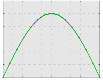
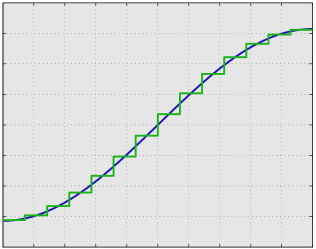
Figure 1.1. Approximation of $-u^{\prime\prime}=f$ by the simplest finite element method. The left plot shows $u$ and the right plot shows $-u^{\prime}$, with the exact solution in blue and the finite element solution in green.

The weak formulation (3) associated to minimization of the functional (2) is not the only variational formulation that can be used for discretization, and in more complicated situations other formulations may bring important advantages. In this simple situation, we may, for example, start by writing the differential equation $-u^{\prime\prime}=f$ as the first order system

$$\sigma=-u^{\prime},\quad\sigma^{\prime}=f.$$

The pair $(\sigma,u)$ can then be characterized variationally as the unique critical point of the functional

$$I(\sigma,u)=\int_{-1}^{1}(\frac{1}{2}\sigma^{2}-u\sigma^{\prime})\,dx+\int_{-1}^{1}fu\,dx$$

over $H^{1}(-1,1)\times L^{2}(-1,1)$. Equivalently, the pair is the solution of the weak formulation: Find $\sigma\in H^{1}(-1,1),u\in L^{2}(-1,1)$ satisfying

$$\int_{-1}^{1}\sigma\tau\,dx-\int_{-1}^{1}u\tau^{\prime}\,dx=0,\quad\tau\in H^{1}(-1,1),$$

$$\int_{-1}^{1}\sigma^{\prime}v\,dx=\int_{-1}^{1}fv\,dx,\quad v\in L^{2}(-1,1).$$

This is called a mixed formulation of the boundary value problem. Note that for the mixed formulation, the Dirichlet boundary condition is implied by the formulation, as can be seen by integration by parts. Note also that in this case the solution is a saddle point of the functional $I$, not an extremum: $I(\sigma,v)\leq I(\sigma,u)\leq I(\tau,u)$ for $\tau\in H^{1}(-1,1)$, $v\in L^{2}(-1,1)$.

Although the mixed formulation is perfectly well-posed, it may easily lead to a discretization which is not. If we apply Galerkin’s method with a simple choice of trial subspaces $\Sigma_{h}\subset H^{1}(-1,1)$ and $V_{h}\subset L^{2}(-1,1)$, we obtain a finite-dimensional linear system, which, however, may be singular, or may become increasingly unstable as the mesh is refined. This concept will be formalized and explored in the next section, but the result of such instability is clearly visible in simple computations. For example, the choice of continuous piecewise linear functions for both $\Sigma_{h}$ and $V_{h}$ leads to a singular linear system. The choice of continuous piecewise linear functions for $\Sigma_{h}$ and piecewise constants for $V_{h}$ leads to stable discretization and good accuracy. However choosing piecewise quadratics for $\Sigma_{h}$ and piecewise constants for $V_{h}$ gives a nonsingular system but unstable approximation (see [25] for further discussion of this example). The dramatic difference between the stable and unstable methods can be seen in Figure 1.2.

 

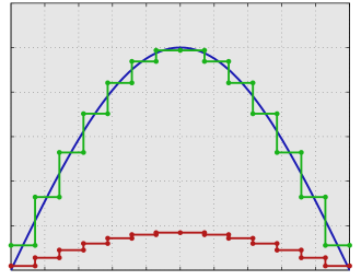
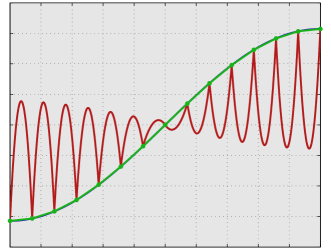
Figure 1.2. Approximation of the mixed formulation for $-u^{\prime\prime}=f$ in one dimension with two choices of elements, piecewise constants for $u$ and piecewise linears for $\sigma$ (a stable method, shown in green), or piecewise constants for $u$ and piecewise quadratics for $\sigma$ (unstable, shown in red). The left plot shows $u$ and the right plot shows $\sigma$, with the exact solution in blue. (In the right plot, the blue curve essentially coincides with the green curve and hence is not visible.)

In one dimension, finding stable pairs of finite dimensional subspaces for the mixed formulation of the two-point boundary value problem is easy. For any integer $r\geq 1$, the combination of continuous piecewise polynomials of degree at most $r$ for $\sigma$ and arbitrary piecewise polynomials of degree at most $r-1$ for $u$ is stable as can be verified via elementary means (and which can be viewed as a very simple application of the theory presented in this paper). In higher dimensions, the problem of finding stable combinations of elements is considerably more complicated. This is discussed in Section 2.3.1 below. In particular, we shall see that the choice of continuous piecewise linear functions for $\sigma$ and piecewise constant functions for $u$ is not stable in more than one dimension. However stable element choices are known for this problem and again may be viewed as a simple application of the finite element exterior calculus developed in this paper.

1.2. The contents of this paper

The brief introduction to the finite element method just given will be continued in Section 2. In particular, there we formalize the notions of consistency and stability and establish their relation to convergence. We shall also give several more computational examples. While seemingly simple, some of these examples may be surprising even to specialists, and they illustrate the difficulty in obtaining good methods and the need for a theoretical framework in which to understand such behaviors.

Like the theory of weak solutions of PDEs, the theory of finite element methods is based on functional analysis and takes its most natural form in a Hilbert space setting. In Section 3 of this paper, we develop an abstract Hilbert space framework which captures key elements of Hodge theory, and can be used to explore the stability of finite element methods. The most basic object in this framework is a cochain complex of Hilbert spaces, referred to as a Hilbert complex. Function spaces of such complexes will occur in the weak formulations of the PDE problems we consider, and the differentials will be differential operators entering into the PDE problem. The most canonical example of a Hilbert complex is the $L^{2}$ de Rham complex of a Riemannian manifold, but it is a far more general object with other important realizations. For example, it allows the definition of spaces of harmonic forms and the proof that they are isomorphic to the cohomology groups. A Hilbert complex includes enough structure to define an abstract Hodge Laplacian, defined from a variational problem with a saddle point structure. However, for these problems to be well–posed, we need the additional property of a closed Hilbert complex, i.e., that the range of the differentials are closed.

In this framework, the finite element spaces used to compute approximate solutions are represented by finite dimensional subspaces of the spaces in the closed Hilbert complex. We identify two key properties of these subspaces: first, they should combine to form a subcomplex of the Hilbert complex, and, second, there should exist a bounded cochain projection from the Hilbert complex to this subcomplex. Under these hypotheses and a minor consistency condition, it is easy to show that the subcomplex inherits the cohomology of the true complex, i.e., that the cochain projections induce an isomorphism from the space of harmonic forms to the space of discrete harmonic forms, and to get an error estimate on the difference between a harmonic form and its discrete counterpart. In the applications, this will be crucial for stable approximation of the PDEs. In fact, a main theme of finite element exterior calculus is that the same two assumptions, the subcomplex property and the existence of a bounded cochain projection, are the natural hypotheses to establish the stability of the corresponding discrete Hodge Laplacian, defined by the Galerkin method.

In Section 4 we look in more depth at the canonical example of the de Rham complex for a bounded domain in Euclidean space, beginning with a brief summary of exterior calculus. We interpret the de Rham complex as a Hilbert complex and discuss the PDEs most closely associated with it. This brings us to the topic of Section 5, the construction of finite element de Rham subcomplexes, which is the heart of finite element exterior calculus and the reason for its name. In this section, we construct finite element spaces of differential forms—piecewise polynomial spaces defined via a simplicial decomposition and specification of shape functions and degrees of freedom—which combine to form a subcomplex of the $L^{2}$ de Rham complex admitting a bounded cochain projection. First we construct the spaces of polynomial differential forms used for shape functions, relying heavily on the Koszul complex and its properties, and then we construct the degrees of freedom. We next show that the resulting finite element spaces can be efficiently implemented, have good approximation properties, and can be combined into de Rham subcomplexes. Finally, we construct bounded cochain projections, and, having verified the hypotheses of the abstract theory, draw conclusions for the finite element approximation of the Hodge Laplacian.

In the final two sections of the paper, we make other applications of the abstract framework. In the last section, we study a differential complex we call the elasticity complex, which is quite different from the de Rham complex. In particular, one of its differentials is a partial differential operator of second order. Via the finite element exterior calculus of the elasticity complex, we have obtained the first stable mixed finite elements using polynomial shape functions for the equations of elasticity, with important applications in solid mechanics.

1.3. Antecedents and related approaches

We now discuss some of the antecedents of finite element exterior calculus and some related approaches. While the first comprehensive view of finite element exterior calculus, and the first use of that phrase, was in the 2006 paper [8], this was certainly not the first intersection of finite element theory and Hodge theory. In 1957, Whitney [88] published his complex of Whitney forms, which is, in our terminology, a finite element de Rham subcomplex. Whitney’s goals were geometric. For example, he used these forms in a proof of de Rham’s theorem identifying the cohomology of a manifold defined via differential forms (de Rham cohomology) with that defined via a triangulation and cochains (simplicial cohomology). With the benefit of hindsight, we may view this, at least in principle, as an early application of finite elements to reduce the computation of a quantity of interest defined via infinite dimensional function spaces and operators, to a finite dimensional computation using piecewise polynomials on a triangulation. The computed quantities are the Betti numbers of the manifold, i.e., the dimensions of the de Rham cohomology spaces. For these integer quantities, issues of approximation and convergence do not play much of a role. The situation is different in the 1976 work of Dodziuk [39] and Dodziuk and Patodi [40], who considered the approximation of the Hodge Laplacian on a Riemannian manifold by a combinatorial Hodge Laplacian, a sort of finite difference approximation defined on cochains with respect to a triangulation. The combinatorial Hodge Laplacian was defined in [39] using the Whitney forms, thus realizing the finite difference operator as a sort of finite element approximation. A key result in [39] was a proof of some convergence properties of the Whitney forms. In [40] the authors applied them to show that the eigenvalues of the combinatorial Hodge Laplacian converge to those of the true Hodge Laplacian. This is indeed a finite element convergence result, as the authors remark. In 1978, Müller [71] further developed this work and used it to prove the Ray–Singer conjecture. This conjecture equates a topological invariant defined in terms of the Riemannian structure with one defined in terms of a triangulation, and was the original goal of [39, 40]. (Cheeger [30] gave a different, independent proof of the Ray–Singer conjecture at about the same time.) Other spaces of finite element differential forms have appeared in geometry as well, especially the differential graded algebra of piecewise polynomial forms on a simplicial complex introduced by Sullivan [83, 84]. Baker [15] calls these Sullivan–Whitney forms, and, in an early paper bringing finite element analysis techniques to bear on geometry, gives a numerical analysis of their accuracy for approximating the eigenvalues of the Hodge Laplacian.

Independently of the work of the geometers, during the 1970s and 1980s numerical analysts and computational engineers reinvented various special cases of the Whitney forms and developed new variants of them to use for the solution of partial differential equations on two and three-dimensional domains. In this work, naturally, implementational issues, rates of convergence, and sharp estimates played a more prominent role than in the geometry literature. The pioneering paper of Raviart and Thomas [76], presented at a finite element conference in 1975, proposed the first stable finite elements for solving the scalar Laplacian in two dimensions using the mixed formulation. The mixed formulation involves two unknown fields, the scalar-valued solution, and an additional vector-valued variable representing its gradient. Raviart and Thomas proposed a family of pairs of finite element spaces, one for each polynomial degree. As was realized later, in the lowest degree case the space they constructed for the vector-valued variable is just the space of Whitney 1-forms, while they used piecewise constants, which are Whitney 2-forms, for the scalar variable. For higher degrees, their elements are the higher order Whitney forms. In three-dimensions, the introduction of Whitney 1- and 2-forms for finite element computations and their higher degree analogues was made by Nédélec [72] in 1980, while the polynomial mixed elements which can be viewed as Sullivan–Whitney forms were introduced as finite elements by Brezzi, Douglas, and Marini [26] in 1985 in two dimensions, and then by Nédélec [72] in 1986 in three dimensions.

In 1988 Bossavit, in a paper in the IEE Transactions on Magnetics [21], made the connection between Whitney’s forms used by geometers and some of the mixed finite element spaces that had been proposed for electromagnetics, inspired in part by Kotiuga’s Ph.D. thesis in electrical engineering [66]. Maxwell’s equations are naturally formulated in terms of differential forms, and the computational electromagnetics community developed the connection between mixed finite elements and Hodge theory in a number of directions. See, in particular, [17, 37, 57, 58, 59, 70].

The methods we derive here are examples of compatible discretization methods, which means that at the discrete level they reproduce, rather than merely approximate, certain essential structures of the continuous problem. Other examples of compatible discretization methods for elliptic PDEs are mimetic finite difference methods [16, 27] including covolume methods [74] and the discrete exterior calculus [38]. In these methods, the fundamental object used to discretize a differential $k$-form is typically a simplicial cochain, i.e., a number is assigned to each $k$-dimensional face of the mesh representing the integral of the $k$-form over the face. This is more of a finite difference, rather than finite element, point of view, recalling the early work of Dodziuk on combinatorial Hodge theory. Since the space of $k$-dimensional simplicial cochains is isomorphic to the space of Whitney $k$-forms, there is a close relationship between these methods and the simplest methods of the finite element exterior calculus. In some simple cases, the methods even coincide. In contrast to the finite element approach, these cochain-based approaches do not naturally generalize to higher order methods. Discretizations of exterior calculus and Hodge theory have also been used for purposes other than solving partial differential equations. For example, discrete forms which are identical or closely related to cochains or the corresponding Whitney forms play an important role in geometric modeling, parameterization, and computer graphics. See for example [50, 54, 56, 87].

1.4. Highlights of the finite element exterior calculus

We close this introduction by highlighting some of the features that are unique or much more prominent in the finite element exterior calculus than in earlier works.

• We work in an abstract Hilbert space setting that captures the fundamental structures of the Hodge theory of Riemannian manifolds, but applies more generally. In fact, the paper proceeds in two parts, first the abstract theory for Hilbert complexes, and then the application to the de Rham complex and Hodge theory and other applications.

• Mixed formulations based on saddle point variational principles play a prominent role. In particular, the algorithms we use to approximate the Hodge Laplacian are based on a mixed formulation, as is the analysis of the algorithms. This is in contrast to the approach in the geometry literature, where the underlying variational principle is a minimization principle. In the case of the simplest elements, the Whitney elements, the two methods are equivalent. That is, the discrete solution obtained by the mixed finite element method using Whitney forms, is the same as obtained by Dodziuk’s combinatorial Laplacian. However the different viewpoint leads naturally to different approaches to the analysis. The use of Whitney forms for the mixed formulation is obviously a consistent discretization, and the key to the analysis is to establish stability (see the next section for the terminology). However, for the minimization principle, it is unclear whether Whitney forms provide a consistent approximation, because they do not belong to the domain of the exterior coderivative, and, as remarked in [40], this greatly complicates the analysis. The results we obtain are both more easily proven and sharper.

• Our analysis is based on two main properties of the subspaces used to discretize the Hilbert complex. First, they can be formed into subcomplexes, which is a key assumption in much of the work we have discussed. Second, there exist a bounded cochain projection from the Hilbert complex to the subcomplex. This is a new feature. In previous work, a cochain projection often played a major role, but it was not bounded, and the existence of bounded cochain projections was not realized. In fact, they exist quite generally (see Theorem 3.7), and we review the construction for the de Rham complex in Section 5.5.

• Since we are interested in actual numerical computations, it is important that our spaces be efficiently implementable. This is not true for all piecewise polynomial spaces. As explained in the next section, finite element spaces are a class of piecewise polynomial spaces that can be implemented efficiently by local computations thanks to the existence of degrees of freedom, and the construction of degrees of freedom and local bases is an important part of the finite element exterior calculus.

• For the same reason, high order piecewise polynomials are of great importance, and all the constructions and analysis of finite element exterior calculus carries through for arbitrary polynomial degree.

• A prominent aspect of the finite element exterior calculus is the role of two families of spaces of polynomial differentials form, ${\mathcal{P}}_{r}\Lambda^{k}$ and ${\mathcal{P}}_{r}^{-}\Lambda^{k}$, where the index $r\geq 1$ denotes the polynomial degree and $k\geq 0$ the form degree. These are the shape functions for corresponding finite element spaces of differential $k$-forms which include, as special cases, the Lagrange finite element family, and most of the stable finite element spaces that have been used to define mixed formulations of the Poisson or Maxwell’s equations. The space ${\mathcal{P}}_{1}^{-}\Lambda^{k}$ is the classical space of Whitney $k$-forms. The finite element spaces based on ${\mathcal{P}}_{r}\Lambda^{k}$ are the spaces of Sullivan–Whitney forms. We show that for each polynomial degree $r$, there are $2^{n-1}$ ways to form these spaces in de Rham subcomplexes for a domain in $n$ dimensions. The unified treatment of the spaces ${\mathcal{P}}_{r}\Lambda^{k}$ and ${\mathcal{P}}_{r}^{-}\Lambda^{k}$, particularly their connections via the Koszul complex, is new to the finite element exterior calculus.

The finite element exterior calculus unifies many of the finite element methods that have been developed for solving PDEs arising in fluid and solid mechanics, electromagnetics, and other areas. Consequently, the methods developed here have been widely implemented and applied in scientific and commercial programs such as GetDP [42], FEniCS [44], EMSolve [45], deal.II [46], Diffpack [61], Getfem++ [77], and NGSolve [78]. We also note that, as part of a recent programming effort connected with the FEniCS project, Logg and Mardal [69] have implemented the full set of finite element spaces developed in this paper strictly following the finite element exterior framework as laid out here and [8].

2. Finite element discretizations

In this section we continue the introduction to the finite element method begun above. We move beyond the case of one dimension, and consider not only the formulation of the method, but also its analysis. To motivate the theory developed later in this paper, we present further examples that illustrate how for some problems, even rather simple ones, deriving accurate finite element methods is not a straightforward process.

2.1. Galerkin methods and finite elements

We consider first a simple problem, which can be discretized in a straightforward way, namely the Dirichlet problem for Poisson’s equation in a polyhedral domain $\Omega\subset\mathbb{R}^{n}$:

(4) $$-\Delta u=f\text{ in }\Omega,\quad u=0\text{ on }\partial\Omega.$$

This is the generalization to $n$ dimensions of the problem (1) discussed in the introduction, and the solution may again be characterized as the minimizer of an energy functional analogous to (2) or as the solution of a weak problem analogous to (3). This leads to discretization just as for the one-dimensional case, by choosing a trial space $V_{h}\subset\mathaccent 23{H}^{1}(\Omega)$ and defining the approximate solution $u_{h}\in V_{h}$ by Galerkin’s method:

$$\int_{\Omega}\operatorname{grad}u_{h}(x)\cdot\operatorname{grad}v(x)\,dx=\int_{\Omega}f(x)v(x)\,dx,\quad v\in V_{h}.$$

As in one dimension, the simplest finite element method is obtained by using the trial space consisting of all piecewise linear functions with respect to a given simplicial triangulation of the domain $\Omega$, which are continuous and vanish on $\partial\Omega$. A key to the efficacy of this finite element method is the existence of a basis for the trial space consisting of functions which are locally supported, i.e., vanish on all but a small number of the elements of the triangulation. See Figure 2.1. Because of this, the coefficient matrix of the linear system is easily computed and is sparse, and so the system can be solved efficiently.

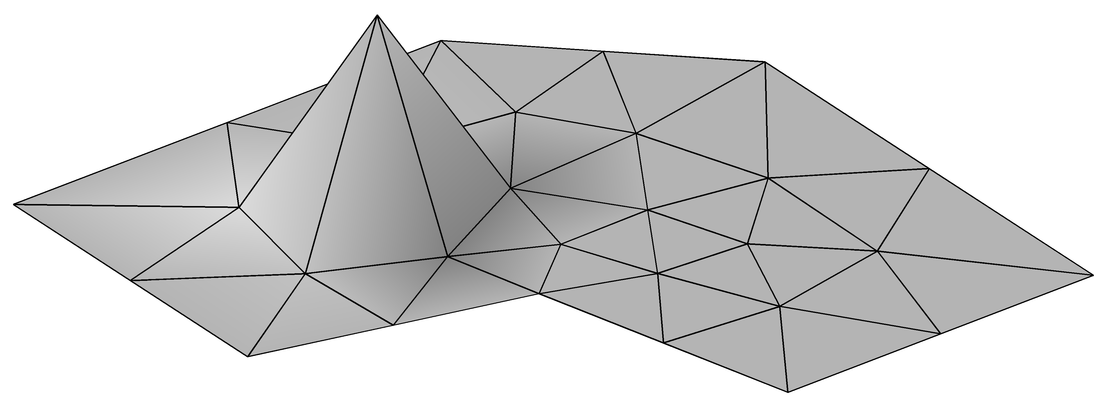
Figure 2.1. A piecewise linear finite element basis function.

More generally, a finite element method is a Galerkin method for which the trial space $V_{h}$ is a space of piecewise polynomial functions which can be obtained by what is called the finite element assembly process. This means that the space can be defined by specifying the triangulation $\mathcal{T}_{h}$ and, for each element $T\in\mathcal{T}_{h}$, a space of polynomial functions on $T$ called the shape functions, and a set of degrees of freedom. By degrees of freedom on $T$, we mean a set of functionals on the space of shape functions, which can be assigned values arbitrarily to determine a unique shape function. In other words, the degrees of freedom form a basis for the dual space of the space of shape functions. In the case of piecewise linear finite elements, the shape functions are of course the linear polynomials on $T$, a space of dimension $n+1$, and the degrees of freedom are the $n+1$ evaluation functionals $p\mapsto p(x)$, where $x$ varies over the vertices of $T$. For the finite element assembly process, we also require that each degree of freedom be associated to a face of some dimension of the simplex $T$. For example, in the case of piecewise linear finite elements, the degree of freedom $p\mapsto p(x)$ is associated to the vertex $x$. Given the triangulation, shape functions, and degrees of freedom, the finite element space $V_{h}$ is defined as the set of functions on $\Omega$ (possibly multivalued on the element boundaries) whose restriction to any $T\in\mathcal{T}_{h}$ belongs to the given space of shape functions on $T$, and for which the degrees of freedom are single-valued in the sense that when two elements share a common face, the corresponding degrees of freedom take on the same value. Returning again to the example of piecewise linear functions, $V_{h}$ is the set of functions which are linear polynomials on each element, and which are single-valued at the vertices. It is easy to see that this is precisely the space of continuous piecewise linear functions, which is a subspace of $H^{1}(\Omega)$. As another example, we could take the shape functions on $T$ to be the polynomials of degree at most $2$, and take as degrees of freedom the functions $p\mapsto p(x)$, $x$ a vertex of $T$, and $p\mapsto\int_{e}p\,ds$, $e$ an edge of $T$. The resulting assembled finite element space is the space of all continuous piecewise quadratics. The finite element assembly process insures the existence of a computable locally supported basis, which is important for efficient implementation.

2.2. Consistency, stability, and convergence

We now turn to the important problem of analyzing the error in the finite element method. To understand when a Galerkin method will produce a good approximation to the true solution, we introduce the standard abstract framework. Let $V$ be a Hilbert space, $B:V\times V\to\mathbb{R}$ a bounded bilinear form, and $F:V\to\mathbb{R}$ a bounded linear form. We assume the problem to be solved can be stated in the form: Find $u\in V$ such that

$$B(u,v)=F(v),\quad v\in V.$$

This problem is called well-posed if for each $F\in V^{*}$, there exists a unique solution $u\in V$ and the mapping $F\mapsto u$ is bounded, or, equivalently, if the operator $L:V\to V^{*}$ given by $\langle Lu,v\rangle=B(u,v)$ is an isomorphism. For the Dirichlet problem for Poisson’s equation,

(5) $$V=\mathaccent 23{H}^{1}(\Omega),\quad B(u,v)=\int_{\Omega}\operatorname{grad}u(x)\cdot\operatorname{grad}v(x)\,dx,\quad F(v)=\int_{\Omega}f(x)v(x)\,dx.$$

A generalized Galerkin method for the abstract problem begins with a finite-dimensional normed space $V_{h}$ (not necessarily a subspace of $V$), a bilinear form $B_{h}:V_{h}\times V_{h}\to R$, and a linear form $F_{h}:V_{h}\to\mathbb{R}$, and defines $u_{h}\in V_{h}$ by

(6) $$B_{h}(u_{h},v)=F_{h}(v),\quad v\in V_{h}.$$

A Galerkin method is the special case of a generalized Galerkin method for which $V_{h}$ is a subspace of $V$ and the forms $B_{h}$ and $F_{h}$ are simply the restrictions of the forms $B$ and $F$ to the subspace. The more general setting is important since it allows the incorporation of additional approximations, such as numerical integration to evaluate the integrals, and also allows for situations in which $V_{h}$ is not a subspace of $V$. Although we do not treat approximations such as numerical integration in this paper, for the fundamental discretization method we study, namely the mixed method for the abstract Hodge Laplacian introduced in Section 3.4, the trial space $V_{h}$ is not a subspace of $V$, since it involves discrete harmonic forms which will not, in general, belong to the space of harmonic forms.

The generalized Galerkin method (6) may be written $L_{h}u_{h}=F_{h}$ where $L_{h}:V_{h}\to V_{h}^{*}$ is given by $\langle L_{h}u,v\rangle=B_{h}(u,v)$, $u,v\in V_{h}$. If the finite-dimensional problem is nonsingular, then we define the norm of the discrete solution operator, $\|L_{h}^{-1}\|_{\mathcal{L}(V_{h}^{*},V_{h})}$, as the stability constant of the method.

Of course, in approximating the original problem determined by $V$, $B$, and $F$, by the generalized Galerkin method given by $V_{h}$, $B_{h}$, and $F_{h}$, we intend that the space $V_{h}$ in some sense approximates $V$ and that the discrete forms $B_{h}$ and $F_{h}$ in some sense approximate $B$ and $F$. This is the essence of consistency. Our goal is to prove that the discrete solution $u_{h}$ approximates $u$ in an appropriate sense (convergence). In order to make these notions precise, we need to compare a function in $V$ to a function in $V_{h}$. To this end, we suppose that there is a restriction operator $\pi_{h}:V\to V_{h}$, so that $\pi_{h}u$ is thought to be close to $u$. Then the consistency error is simply $L_{h}\pi_{h}u-F_{h}$ and the error in the generalized Galerkin method which we wish to control is $\pi_{h}u-u_{h}$. We immediately get a relation between the error and the consistency error

$$\pi_{h}u-u_{h}=L_{h}^{-1}(L_{h}\pi_{h}u-F_{h}),$$

and so the norm of the error is bounded by the product of the stability constant and the norm of the consistency error:

$$\|\pi_{h}u-u_{h}\|_{V_{h}}\leq\|L_{h}^{-1}\|_{\mathcal{L}(V_{h}^{*},V_{h})}\|L_{h}\pi_{h}u-F_{h}\|_{V^{*}_{h}}.$$

Stated in terms of the bilinear form $B_{h}$, the norm of the consistency error can be written

$$\|L_{h}\pi_{h}u-F_{h}\|_{V^{*}_{h}}=\sup_{0\neq v\in V_{h}}\frac{B_{h}(\pi_{h}u,v)-F_{h}(v)}{\|v\|_{V_{h}}}.$$

As for stability, the finite dimensional problem is nonsingular if and only if

$$\gamma_{h}:=\inf_{0\neq u\in V_{h}}\sup_{0\neq v\in V_{h}}\frac{B_{h}(u,v)}{\|u\|_{V_{h}}\|v\|_{V_{h}}}>0,$$

and the stability constant is then given by $\gamma_{h}^{-1}$.

Often we consider a sequence of spaces $V_{h}$ and forms $B_{h}$ and $F_{h}$ where we think of $h>0$ as an index accumulating at $0$. The corresponding generalized Galerkin method is consistent if the $V_{h}$ norm of the consistency error tends to zero with $h$ and it is stable if the stability constant $\gamma_{h}^{-1}$ is uniformly bounded. For a consistent, stable generalized Galerkin method, $\|\pi_{h}u-u_{h}\|_{V_{h}}$ tends to zero, i.e., the method is convergent.

In the special case of a Galerkin method, we can bound the consistency error

$$\sup_{0\neq v\in V_{h}}\frac{B_{h}(\pi_{h}u,v)-F_{h}(v)}{\|v\|_{V}}=\sup_{0\neq v\in V_{h}}\frac{B(\pi_{h}u-u,v)}{\|v\|_{V}}\leq\|B\|\|\pi_{h}u-u\|_{V}.$$

In this case it is natural to choose the restriction $\pi_{h}$ to be the orthogonal projection onto $V_{h}$, and so the consistency error is bounded by the norm of the bilinear form times the error in the best approximation of the solution. Thus we obtain

$$\|\pi_{h}u-u_{h}\|_{V}\leq\gamma_{h}^{-1}\|B\|\inf_{v\in V_{h}}\|u-v\|_{V}.$$

Combining this with the triangle inequality, we obtain the basic error estimate for Galerkin methods

(7) $$\|u-u_{h}\|_{V}\leq(1+\gamma_{h}^{-1}\|B\|)\inf_{v\in V_{h}}\|u-v\|_{V}.$$

(In fact, in this Hilbert space setting, the quantity in parentheses can be replaced with $\gamma_{h}^{-1}\|B\|$, see [89].) Note that a Galerkin method is consistent as long as the sequence of subspaces $V_{h}$ is approximating in $V$ in the sense that

(8) $$\lim_{h\to 0}\inf_{v\in V_{h}}\|u-v\|_{V}=0,\quad u\in V.$$

A consistent, stable Galerkin method converges, and the approximation given by the method is quasioptimal, i.e., up to multiplication by a constant, it is as good as the best approximation in the subspace.

In practice, it can be quite difficult to show that the finite dimensional problem is nonsingular and to bound the stability constant, but there is one important case in which it is easy. Namely when the form $B$ is coercive, i.e., there is a positive constant $\alpha$ for which

$$B(v,v)\geq\alpha\|v\|_{V}^{2},\quad v\in V,$$

and so $\gamma_{h}\geq\alpha$. The bilinear form (5) for Poisson’s equation is coercive, as follows from Poincaré’s inequality. This explains, and can be used to prove, the good convergence behavior of the method depicted in Figure 1.1.

2.3. Computational examples

2.3.1. Mixed formulation of the Laplacian

For an example of a problem that fits in the standard abstract framework with a noncoercive bilinear form, we take the mixed formulation of the Dirichlet problem for Poisson’s equation, already introduced in one dimension in Section 1.1. Just as there, we begin by writing Poisson’s equation as the first order system

(9) $$\sigma=-\operatorname{grad}u,\quad\operatorname{div}\sigma=f.$$

The pair $(\sigma,u)$ can again be characterized variationally as the unique critical point (a saddle point) of the functional

$$I(\sigma,u)=\int_{\Omega}(\frac{1}{2}\sigma\cdot\sigma-u\operatorname{div}\sigma)\,dx+\int_{\Omega}fu\,dx$$

over $H(\operatorname{div};\Omega)\times L^{2}(\Omega)$ where $H(\operatorname{div};\Omega)=\{\sigma\in L^{2}(\Omega):\operatorname{div}\sigma\in L^{2}(\Omega)\}$. Equivalently, it solves the weak problem: Find $\sigma\in H(\operatorname{div};\Omega),u\in L^{2}(\Omega)$ satisfying

$$\int_{\Omega}\sigma\cdot\tau\,dx-\int_{\Omega}u\operatorname{div}\tau\,dx=0,\quad\tau\in H(\operatorname{div};\Omega),$$

$$\int_{\Omega}\operatorname{div}\sigma v\,dx=\int_{\Omega}fv\,dx,\quad v\in L^{2}(\Omega).$$

This mixed formulation of Poisson’s equation fits in the abstract framework if we define $V=H(\operatorname{div};\Omega)\times L^{2}(\Omega)$,

$$B(\sigma,u;\tau,v)=\int_{\Omega}\sigma\cdot\tau\,dx-\int_{\Omega}u\operatorname{div}\tau\,dx+\int_{\Omega}\operatorname{div}\sigma v\,dx,\quad F(\tau,v)=\int_{\Omega}fv\,dx.$$

In this case the bilinear form $B$ is not coercive, and so the choice of subspaces and the analysis is not so simple as for the standard finite element method for Poisson’s equation, a point we already illustrated in the one-dimensional case.

Finite element discretizations based on such saddle point variational principles are called mixed finite element methods. Thus a mixed finite element for Poisson’s equation is obtained by choosing subspaces $\Sigma_{h}\subset H(\operatorname{div};\Omega)$ and $V_{h}\subset L^{2}(\Omega)$ and seeking a critical point of $I$ over $\Sigma_{h}\times V_{h}$. The resulting Galerkin method has the form: Find $\sigma_{h}\in\Sigma_{h},u_{h}\in V_{h}$ satisfying

$$\int_{\Omega}\sigma_{h}\cdot\tau\,dx-\int_{\Omega}u_{h}\operatorname{div}\tau\,dx=0,\quad\tau\in\Sigma_{h},\quad\int_{\Omega}\operatorname{div}\sigma_{h}v\,dx=\int_{\Omega}fv\,dx,\quad v\in V_{h}.$$

This again reduces to a linear system of algebraic equations.

Since the bilinear form is not coercive, it is not automatic that the linear system is nonsingular, i.e., that for $f=0$, the only solution is $\sigma_{h}=0$, $u_{h}=0$. Choosing $\tau=\sigma_{h}$ and $v=u_{h}$ and adding the discretized variational equations, it follows immediately that when $f=0$, $\sigma_{h}=0$. However, $u_{h}$ need not vanish unless the condition that $\int_{\Omega}u_{h}\operatorname{div}\tau\,dx=0$ for all $\tau\in\Sigma_{h}$ implies that $u_{h}=0$. In particular, this requires that $\dim(\operatorname{div}\Sigma_{h})\geq\dim V_{h}$. Thus, even nonsingularity of the approximate problem depends on a relationship between the two finite dimensional spaces. Even if the linear system is nonsingular, there remains the issue of stability, i.e., a uniform bound on the inverse operator.

As mentioned earlier, the combination of continous piecewise linear elements for $\sigma$ and piecewise constants for $u$ is not stable in two dimensions. The simplest stable elements use the piecewise constants for $u$, and the lowest order Raviart-Thomas elements for $\sigma$. These are finite elements defined with respect to a triangular mesh by shape functions of the form $(a+bx_{1},c+bx_{2})$ and one degree of freedom for each edge $e$, namely $\sigma\mapsto\int_{e}\sigma\cdot n\,ds$. We show in Fig. 2.2 below two numerical computations that demonstrate the difference between an unstable and stable choice of elements for this problem. The stable method accurately approximates the true solution $u=x(1-x)y(1-y)$ on $(0,1)\times(0,1)$ with a piecewise constant, while the unstable method is wildly oscillatory.

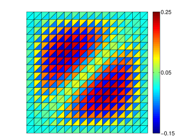
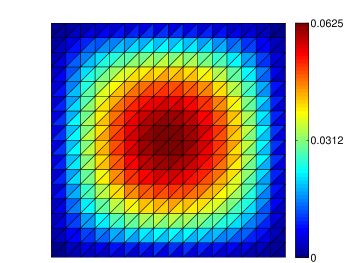
Figure 2.2. Approximation of the mixed formulation for Poisson’s equation using piecewise constants for $u$ and for $\sigma$ either continuous piecewise linears (left), or Raviart–Thomas elements (right). The plotted quantity is $u$ in each case.

This problem is a special case of the Hodge Laplacian with $k=n$ as discussed briefly in Section 4.2; see especially Section 4.2.4. The error analysis for a variety of finite element methods for this problem, including the Raviart–Thomas elements, is thus a special case of the general theory of this paper, yielding the error estimates in Section 5.6.

2.3.2. The vector Laplacian on a nonconvex polygon

Given the subtlety of finding stable pairs of finite element spaces for the mixed variational formulation of Poisson’s equation, we might choose to avoid this formulation, in favor of the standard formulation, which leads to a coercive bilinear form. However, while the standard formulation is easy to discretize for Poisson’s equation, additional issues arise already if we try to discretize the vector Poisson equation. For a domain $\Omega$ in $\mathbb{R}^{3}$ with unit outward normal $n$, this is the problem

(10) $$-\operatorname{grad}\operatorname{div}u+\operatorname{curl}\operatorname{curl}u=f,\text{ in }\Omega,\quad u\cdot n=0,\quad\operatorname{curl}u\times n=0,\quad\text{ on }\partial\Omega.$$

The solution of this problem can again be characterized as the minimizer of an appropriate energy functional,

(11) $$J(u)=\frac{1}{2}\int_{\Omega}(|\operatorname{div}u|^{2}+|\operatorname{curl}u|^{2})\,dx-\int_{\Omega}f\cdot u\,dx,$$

but this time over the space $H(\operatorname{curl};\Omega)\cap\mathaccent 23{H}(\operatorname{div};\Omega)$, where $H(\operatorname{curl};\Omega)=\{u\in L^{2}(\Omega)\,|\,\operatorname{curl}u\in L^{2}(\Omega)\}$ and $\mathaccent 23{H}(\operatorname{div};\Omega)=\{u\in H(\operatorname{div};\Omega)\,|\,u\cdot n=0\ \text{on}\ \partial\Omega\}$ with $H(\operatorname{div};\Omega)$ defined above. This problem is associated to a coercive bilinear form, but a standard finite element method based on a trial subspace of the energy space $H(\operatorname{curl};\Omega)\cap\mathaccent 23{H}(\operatorname{div};\Omega)$, e.g., using continuous piecewise linear vector functions, is very problematic. In fact, as we shall illustrate shortly, if the domain $\Omega$ is a nonconvex polyhedron, for almost all $f$ the Galerkin method solution will converge to a function that is not the true solution of the problem! The essence of this unfortunate situation is that any piecewise polynomial subspace of $H(\operatorname{curl};\Omega)\cap\mathaccent 23{H}(\operatorname{div};\Omega)$ is a subspace of $H^{1}(\Omega)\cap\mathaccent 23{H}(\operatorname{div};\Omega)$, and this space is a closed subspace of $H(\operatorname{curl};\Omega)\cap\mathaccent 23{H}(\operatorname{div};\Omega)$. For a nonconvex polyhedron, it is a proper closed subspace and generally the true solution will not belong to it, due to a singularity at the reentrant corner. Thus the method, while stable, is inconsistent. For more on this example, see [35].

An accurate approximation of the vector Poisson equation can be obtained from a mixed finite element formulation, based on the system:

$$\sigma=-\operatorname{div}u,\quad\operatorname{grad}\sigma+\operatorname{curl}\operatorname{curl}u=f\text{ in }\Omega,\quad u\cdot n=0,\quad\operatorname{curl}u\times n=0\text{ on }\partial\Omega.$$

Writing this system in weak form, we obtain the mixed formulation of the problem: Find $\sigma\in H^{1}(\Omega)$, $u\in H(\operatorname{curl};\Omega)$ satisfying

$$\int_{\Omega}\sigma\tau\,dx-\int_{\Omega}u\cdot\operatorname{grad}\tau\,dx=0,\quad\tau\in H^{1}(\Omega),$$

$$\int_{\Omega}\operatorname{grad}\sigma\cdot v\,dx+\int_{\Omega}\operatorname{curl}u\cdot\operatorname{curl}v\,dx=\int_{\Omega}f\cdot v\,dx,\quad v\in H(\operatorname{curl};\Omega).$$

In contrast to a finite element method based on minimizing the energy (11), a finite element approximation based on the mixed formulation uses separate trial subspaces of $H^{1}(\Omega)$ and $H(\operatorname{curl};\Omega)$, rather than a single subspace of the intersection $H(\operatorname{curl};\Omega)\cap\mathaccent 23{H}(\operatorname{div};\Omega)$.

We now illustrate the nonconvergence of a Galerkin method based on energy minimization and the convergence of one based on the mixed formulation, via computations in two space dimensions (so now the curl of a vector $u$ is the scalar $\partial u_{2}/\partial x_{1}-\partial u_{1}/\partial x_{2}$). For the trial subspaces we make the simplest choices: for the former method we use continuous piecewise linear functions and for the mixed method we use continuous piecewise linear functions to approximate $\sigma\in H^{1}(\Omega)$ and a variant of the lowest order Raviart–Thomas elements, for which the shape functions are the infinitesimal rigid motions $(a-bx_{2},c+bx_{1})$ and the degrees of freedom are the tangential moments $u\mapsto\int_{e}u\cdot s\,ds$ for $e$ an edge. The discrete solutions obtained by the two methods for the problem when $f=(-1,0)$ are shown in Figure 2.3. As we shall show later in this paper, the mixed formulation gives an approximation that provably converges to the true solution, while, as can be seen from comparing the two plots, the first approximation scheme gives a completely different (and therefore inaccurate) result.

  

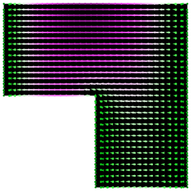
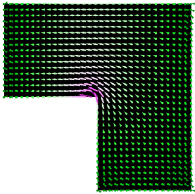
Figure 2.3. Approximation of the vector Laplacian by the standard finite element method (left) and a mixed finite element method (right). The former method totally misses the singular behavior of the solution near the reentrant corner.

This problem is again a special case of the Hodge Laplacian, now with $k=1$. See Section 4.2.2. The error analysis thus falls within the theory of this paper, yielding estimates as in Section 5.6.

2.3.3. The vector Laplacian on an annulus

In the example just considered, the failure of a standard Galerkin method based on energy minimization to solve the vector Poisson equation was related to the reentrant corner of the domain and the resulting singular behavior of the solution. A quite different failure mode for this method occurs if we take a domain which is smoothly bounded, but not simply connected, e.g., an annulus. In that case, as discussed below in Section 3.2, the boundary value problem (10) is not well-posed except for special values of the forcing function $f$. In order to obtain a well-posed problem, the differential equation should be solved only modulo the space of harmonic vector fields (or harmonic 1-forms)—which is a one-dimensional space for the annulus—and the solution should be rendered unique by enforcing orthogonality to the harmonic vector fields. If we choose the annulus with radii $1/2$ and $1$, and forcing function $f=(0,x)$, the resulting solution, which can be computed accurately with a mixed formulation falling within the theory of this paper, is displayed on the right in Figure 2.4. However, the standard Galerkin method does not capture the non-uniqueness and computes the discrete solution shown on the left of the same figure, which is dominated by an approximation of the harmonic vector field, and so is nothing like the true solution.

  

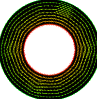
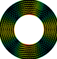
Figure 2.4. Approximation of the vector Laplacian on an annulus. The true solution shown here on the right in an (accurate) approximation by a mixed method. It is orthogonal to the harmonic fields, and satisfies the differential equation only modulo harmonic fields. The standard Galerkin solution using continuous piecewise linear vector fields shown on the left, is totally different.

2.3.4. The Maxwell eigenvalue problem

Another situation where a standard finite element method gives unacceptable results, but a mixed method succeeds, arises in the approximation of elliptic eigenvalue problems related to the vector Laplacian or Maxwell’s equation. This will be analyzed in detail later in this paper, and here we only present a simple but striking computational example. Consider the eigenvalue problem for the vector Laplacian discussed above, which we write in mixed form as: Find nonzero $(\sigma,u)\in H^{1}(\Omega)\times H(\operatorname{curl};\Omega)$ and $\lambda\in\mathbb{R}$ satisfying

(12) $$\begin{gathered}\int_{\Omega}\sigma\cdot\tau\,dx-\int_{\Omega}\operatorname{grad}\tau\cdot u\,dx=0,\quad\tau\in H^{1}(\Omega).\\ \int_{\Omega}\operatorname{grad}\sigma\cdot v\,dx+\int_{\Omega}\operatorname{curl}u\cdot\operatorname{curl}v\,dx=\lambda\int_{\Omega}u\cdot v\,dx,\quad v\in H(\operatorname{curl};\Omega).\end{gathered}$$

As explained in Section 3.6.1, this problem can be split into two subproblems. In particular, if $0\neq u\in H(\operatorname{curl};\Omega)$ and $\lambda\in\mathbb{R}$ solves the eigenvalue problem

(13) $$\int_{\Omega}\operatorname{curl}u\cdot\operatorname{curl}v\,dx=\lambda\int_{\Omega}u\cdot v\,dx,\quad v\in H(\operatorname{curl};\Omega),$$

and $\lambda$ is not equal to zero, then $(\sigma,u)$, $\lambda$ is an eigenpair for (12) with $\sigma=0$.

We now consider the solution of the eigenvalue problem (13), with two different choices of trial subspaces in $H(\operatorname{curl};\Omega)$. Again, to make our point it is enough to consider a two dimensional case, and we consider the solution of (13) with $\Omega$ a square of side length $\pi$. For this domain, the positive eigenvalues can be computed by separation of variables. They are of the form $m^{2}+n^{2}$ with $m$ and $n$ integers: $1,1,2,4,4,5,5,8,\ldots$. If we approximate (13) using the space of continuous piecewise linear vector fields as the trial subspace of $H(\operatorname{curl};\Omega)$, the approximation fails badly. This is shown for an unstructured mesh in Figure 2.5 and for a structured crisscross mesh in Figure 2.6, where the nonzero discrete eigenvalues are plotted. Note the very different mode of failure for the two mesh types. For more discussion of the spurious eigenvalues arising using continuous piecewise linear vector fields on a crisscross mesh see [20]. By contrast, if we use the lowest order Raviart–Thomas approximation of $H(\operatorname{curl};\Omega)$, as shown on the right of Figure 2.5, we obtain a provably good approximation for any mesh. This is a very simple case of the general eigenvalue approximation theory presented in Section 3.6 below.

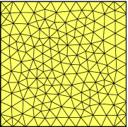
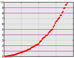
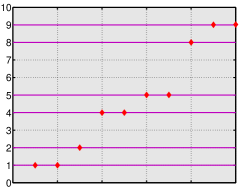
Figure 2.5. Approximation of the nonzero eigenvalues of (13) on an unstructured mesh of the square (left) using continuous piecewise linear finite elements (middle) and Raviart–Thomas elements (right). For the former, the discrete spectrum looks nothing like the true spectrum, while for the later it is very accurate.

  

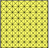
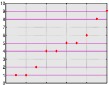
Figure 2.6. Approximation of the nonzero eigenvalues of (13) using continuous piecewise linear elements on the structured mesh shown. The first seven discrete nonzero eigenvalues converge to true eigenvalues, but the eighth converges to a spurious value.

3. Hilbert complexes and their approximation

In this section, we construct a Hilbert space framework for finite element exterior calculus. The most basic object in this framework is a Hilbert complex, which extracts essential features of the $L^{2}$ de Rham complex. Just as the Hodge Laplacian is naturally associated with the de Rham complex, there is a system of variational problems, which we call the abstract Hodge Laplacian, associated to any Hilbert complex. Using a mixed formulation we prove that these abstract Hodge Laplacian problems are well-posed. We next consider approximation of Hilbert complexes using finite dimensional subspaces. Our approach emphasizes two key properties, the subcomplex property and the existence of bounded cochain projections. These same properties prove to be precisely what is needed both to show that the approximate Hilbert complex accurately reproduces geometrical quantities associated to the complex, like cohomology spaces, and also to obtain error estimates for the approximation of the abstract Hodge Laplacian source and eigenvalue problems, which is our main goal in this section. In the following section of the paper we will derive finite element subspaces in the concrete case of the de Rham complex and verify the hypotheses needed to apply the results of this section.

Although the $L^{2}$ de Rham complex is the canonical example of a Hilbert complex, there are many others. In this paper, in Section 6 we consider some variations of de Rham complex that allow us to treat more general PDEs and boundary value problems. In the final section we briefly discuss the equations of elasticity, for which a very different Hilbert complex, in which one of the differentials is a second order PDE, is needed. Another useful feature of Hilbert complexes, is that a subcomplex of Hilbert complex is again such, and so the properties we establish for them apply not only at the continuous, but also at the discrete level.

3.1. Basic definitions

We begin by recalling some basic definitions of homological algebra and functional analysis and establishing some notation.

3.1.1. Cochain complexes

Consider a cochain complex $(V,d)$ of vector spaces, i.e., a sequence of vector spaces $V^{k}$ and linear maps $d^{k}$, called the differentials:

$$\cdots\to V^{k-1}\xrightarrow{d^{k-1}}V^{k}\xrightarrow{d^{k}}V^{k+1}\to\cdots$$

with $d^{k}\circ d^{k-1}=0$. Equivalently, we may think of such a complex as the graded vector space $V=\bigoplus V^{k}$, equipped with a graded linear operator $d:V\to V$ of degree $+1$ satisfying $d\circ d=0$. A chain complex differs from a cochain complex only in that the indices decrease. All the complexes we consider are nonnegative and finite, meaning that $V^{k}=0$ whenever $k$ is negative or sufficiently large.

Given a cochain complex $(V,d)$, the elements of the null space $\mathfrak{Z}^{k}=\mathfrak{Z}^{k}(V,d)$ of $d^{k}$ are called the $k$-cocycles and the elements of the range $\mathfrak{B}^{k}=\mathfrak{B}^{k}(V,d)$ of $d^{k-1}$ the $k$-coboundaries. The $k$th cohomology group is defined to be the quotient space $\mathfrak{Z}^{k}/\mathfrak{B}^{k}$.

Given two cochain complexes $(V,d)$ and $(V^{\prime},d^{\prime})$, a set of linear maps $f^{k}:V^{k}\to V^{\prime k}$ satisfying $d^{\prime k}f^{k}=f^{k+1}d^{k}$ (i.e., a graded linear map $f:V\to V^{\prime}$ of degree $0$ satisfying $d^{\prime}f=fd$) is called a cochain map. When $f$ is a cochain map, $f^{k}$ maps $k$-cocycles to $k$-cocycles and $k$-coboundaries to $k$-coboundaries, and hence induces a map $\bar{f}$ on the cohomology spaces. This map is functorial, i.e., it respects composition.

Let $(V,d)$ be a cochain complex and $(V_{h},d)$ a subcomplex. In other words, $V_{h}^{k}$ is a subspace of $V^{k}$ and $d^{k}V_{h}^{k}\subset V_{h}^{k+1}$. Then the inclusion $i_{h}:V_{h}\to V$ is a cochain map and so induces a map of cohomology. If there exists a cochain projection of $V$ onto $V_{h}$, i.e., a cochain map $\pi_{h}$ such that $\pi_{h}^{k}:V^{k}\to V_{h}^{k}$ leaves the subspace $V_{h}^{k}$ invariant, then $\pi_{h}\circ i_{h}=\operatorname{id}_{V_{h}}$, so $\bar{\pi}_{h}\circ\bar{i}_{h}=\operatorname{id}_{\mathfrak{Z}_{h}^{k}/\mathfrak{B}_{h}^{k}}$ (where $\mathfrak{Z}_{h}^{k}:=\mathfrak{Z}^{k}(V_{h},d)$ and similarly for $\mathfrak{B}_{h}^{k}$). We conclude that in this case $\bar{i}_{h}$ is injective and $\bar{\pi}_{h}$ is surjective. In particular, the dimension of the cohomology spaces of the subcomplex is at most that of the supercomplex.

3.1.2. Closed operators on Hilbert space

This material can be found in many places, e.g., [64, Chapter III, § 5 and Chapter IV, § 5.2] or [90, Chapter II, § 6 and Chapter VII].

By an operator $T$ from a Hilbert space $X$ to a Hilbert space $Y$, we mean a linear operator from a subspace $V$ of $X$, called the domain of $T$, into $Y$. The operator $T$ is not necessarily bounded and the domain $V$ is not necessarily closed. We say that the operator $T$ is closed if its graph $\{\,(x,Tx)\,|\,x\in V\,\}$ is closed in $X\times Y$. We endow the domain $V$ with the graph norm inner product,

$$\langle v,w\rangle_{V}=\langle v,w\rangle_{X}+\langle Tv,Tw\rangle_{Y}.$$

It is easy to check that this makes $V$ a Hilbert space (i.e., complete), if and only if $T$ is closed, and moreover, that $T$ is a bounded operator from $V$ to $Y$. Of course, the null space of $T$ is the set of elements of its domain which it maps to $0$, and the range of $T$ is $T(V)$. The null space of a closed operator from $X$ to $Y$ is a closed subspace of $X$, but its range need not be closed in $Y$ (even if the operator is defined on all of $X$ and is bounded).

The operator $T$ is said to be densely defined if its domain $V$ is dense in $X$. In this case the adjoint operator $T^{*}$ from $Y$ to $X$ is defined to be the operator whose domain consists of all $y\in Y$ for which there exists $x\in X$ with

$$\langle x,v\rangle_{X}=\langle y,Tv\rangle_{Y},\quad v\in V,$$

in which case $T^{*}y=x$ (well-defined since $V$ is dense). If $T$ is closed and densely defined, then $T^{*}$ is as well and $T^{**}=T$. Moreover, the null space of $T^{*}$ is the orthogonal complement of the range of $T$ in $Y$. Finally, by the closed range theorem, the range of $T$ is closed in $Y$ if and only if the range of $T^{*}$ is closed in $X$.

If the range of a closed linear operator is of finite codimension, i.e., $\dim Y/T(V)<\infty$, then the range is closed [60, Lemma 19.1.1].

3.1.3. Hilbert complexes

A Hilbert complex is a sequence of Hilbert spaces $W^{k}$ and closed, densely-defined linear operators $d^{k}$ from $W^{k}$ to $W^{k+1}$ such that the range of $d^{k}$ is contained in the domain of $d^{k+1}$ and $d^{k+1}\circ d^{k}=0$. A Hilbert complex is bounded if, for each $k$, $d^{k}$ is a bounded linear operator from $W^{k}$ to $W^{k+1}$. In other words, a bounded Hilbert complex is a cochain complex in the category of Hilbert spaces. A Hilbert complex is closed if for each $k$, the range of $d^{k}$ is closed in $W^{k+1}$. A Fredholm complex is a Hilbert complex for which the range of $d^{k}$ is finite codimensional in the null space of $d^{k+1}$ (and so is closed). Hilbert and Fredholm complexes have been discussed by various authors working in geometry and topology. Brüning and Lesch [28] have advocated for them as an abstraction of elliptic complexes on manifolds and applied them to spectral geometry on singular spaces. Glotko [53] used them to define a generalization of Sobolev spaces on Riemannian manifolds and study their compactness properties and Gromov and Shubin [55] to define topological invariants of manifolds.

Associated to any Hilbert complex $(W,d)$ is a bounded Hilbert complex $(V,d)$, called the domain complex, for which the space $V^{k}$ is the domain of $d^{k}$, endowed with the inner product associated to the graph norm:

$$\langle u,v\rangle_{V^{k}}=\langle u,v\rangle_{W^{k}}+\langle d^{k}u,d^{k}v\rangle_{W^{k+1}}.$$

Then $d^{k}$ is a bounded linear operator from $V^{k}$ to $V^{k+1}$, and so $(V,d)$ is indeed a bounded Hilbert complex. The domain complex is closed or Fredholm if and only if the original complex $(W,d)$ is.

Of course, for a Hilbert complex $(W,d)$, we have the null spaces and ranges $\mathfrak{Z}^{k}$ and $\mathfrak{B}^{k}$. Utilizing the inner product, we define the space of harmonic forms $\mathfrak{H}^{k}=\mathfrak{Z}^{k}\cap\mathfrak{B}^{k\perp}$, the orthogonal complement of $\mathfrak{B}^{k}$ in $\mathfrak{Z}^{k}$. It is isomorphic to the reduced cohomology space $\mathfrak{Z}^{k}/\overline{\mathfrak{B}^{k}}$ or, for a closed complex, to the cohomology space $\mathfrak{Z}^{k}/\mathfrak{B}^{k}$. For a closed Hilbert complex, we immediately obtain the Hodge decomposition

(14) $$W^{k}=\mathfrak{B}^{k}\oplus\mathfrak{H}^{k}\oplus\mathfrak{Z}^{k\perp_{W}}.$$

For the domain complex $(V,d)$, the null space, range, and harmonic forms are the same spaces as for the original complex, and the Hodge decomposition is

$$V^{k}=\mathfrak{B}^{k}\oplus\mathfrak{H}^{k}\oplus\mathfrak{Z}^{k\perp_{V}}.$$

The third summand, $\mathfrak{Z}^{k\perp_{V}}=\mathfrak{Z}^{k\perp_{W}}\cap V^{k}$.

Continuing to use the Hilbert space structure, we define the dual complex $(W,d^{*})$, which is a Hilbert chain complex rather than cochain complex. The dual complex uses the same spaces $W^{i}$, with the differential $d^{*}_{k}$ being the adjoint of $d^{k-1}$, so $d^{*}_{k}$ is a closed, densely-defined operator from $W^{k}$ to $W^{k-1}$, whose domain we denote by $V^{*}_{k}$. The dual complex is closed or bounded if and only if the original complex is. We denote by $\mathfrak{Z}^{*}_{k}=\mathfrak{B}^{k\perp_{W}}$ the null space of $d^{*}_{k}$, and by $\mathfrak{B}^{*}_{k}$ the range of $d^{*}_{k+1}$. Thus $\mathfrak{H}^{k}=\mathfrak{Z}^{k}\cap\mathfrak{Z}^{*}_{k}$ is the space of harmonic forms both for the original complex and the dual complex. Since $\mathfrak{Z}^{k\perp_{W}}=\mathfrak{B}^{*}_{k}$, the Hodge decomposition (14) can be written

(15) $$W^{k}=\mathfrak{B}^{k}\oplus\mathfrak{H}^{k}\oplus\mathfrak{B}^{*}_{k}.$$

We henceforth simply write $\mathfrak{Z}^{k\perp}$ for $\mathfrak{Z}^{k\perp_{V}}$.

Let $(W,d)$ be a closed Hilbert complex with domain complex $(V,d)$. Then $d^{k}$ is a bounded bijection from $\mathfrak{Z}^{k\perp}$ to the Hilbert space $\mathfrak{B}^{k+1}$ and hence, by Banach’s bounded inverse theorem, there exists a constant $c_{P}$ such that

(16) $$\|v\|_{V}\leq c_{P}\|d^{k}v\|_{W},\quad v\in\mathfrak{Z}^{k\perp},$$

which we refer to as a Poincaré inequality. We remark that the condition that $\mathfrak{B}^{k}$ is closed is not only sufficient to obtain (16), but also necessary.

The subspace $V^{k}\cap V^{*}_{k}$ of $W^{k}$ is a Hilbert space with the norm

$$\|v\|_{V\cap V^{*}}^{2}=\|v\|_{V}^{2}+\|v\|_{V^{*}}^{2}=2\|v\|_{W}^{2}+\|d^{k}v\|_{W}^{2}+\|d_{k}^{*}v\|_{W}^{2},$$

and is continuously included in $W^{k}$. We say that the Hilbert complex $(W,d)$ has the compactness property if $V^{k}\cap V^{*}_{k}$ is dense in $W^{k}$ and the inclusion is a compact operator. Restricted to the space $\mathfrak{H}^{k}$ of harmonic forms, the $V^{k}\cap V^{*}_{k}$ norm is equal to the $W^{k}$ norm (times $\sqrt{2}$). Therefore the compactness property implies that the inclusion of $\mathfrak{H}^{k}$ into itself is compact, so $\mathfrak{H}^{k}$ is finite dimensional. In summary, for Hilbert complexes, $\text{compactness property}\implies\text{Fredholm}\implies\text{closed}$.

3.2. The abstract Hodge Laplacian and the mixed formulation

Given a Hilbert complex $(W,d)$, the operator $L=dd^{*}+d^{*}d$ is an unbounded operator $W^{k}\to W^{k}$ called, in the case of the de Rham complex, the Hodge Laplacian. We refer to it as the abstract Hodge Laplacian in the general situation. Its domain is

$$D_{L}=\{\,u\in V^{k}\cap V^{*}_{k}\,|\,du\in V^{*}_{k+1},d^{*}u\in V^{k-1}\,\}.$$

If $u$ solves $Lu=f$, then

(17) $$\langle du,dv\rangle+\langle d^{*}u,d^{*}v\rangle=\langle f,v\rangle,\quad v\in V^{k}\cap V^{*}_{k}.$$

Note that, in this equation, and henceforth, we use $\langle\,\cdot\,,\,\cdot\,\rangle$ and $\|\,\cdot\,\|$ without subscripts, meaning the inner product and norm in the appropriate $W^{k}$ space.

The harmonic functions measure the extent to which the Hodge Laplace problem (17) is well-posed. The solutions to the homogeneous problem ($f=0$) are precisely the functions in $\mathfrak{H}^{k}$. Moreover, a necessary condition for a solution to exist for non-zero $f\in W^{k}$ is that $f\perp\mathfrak{H}^{k}$.

For computational purposes, a formulation of the Hodge Laplacian based on (17) may be problematic, even when there are no harmonic forms, because it may not be possible to construct an efficient finite element approximation for the space $V^{k}\cap V^{*}_{k}$. We have already seen an example of this in the discussion of the approximation of a boundary value problem for the vector Laplacian in Section 2.3.2. Instead we introduce another formulation, which is a generalization of the mixed formulation discussed in Section 2 and which, simultaneously, accounts for the nonuniqueness associated with harmonic forms. With $(W,d)$ a Hilbert complex, $(V,d)$ the associated domain complex, and $f\in W^{k}$ given, we define the mixed formulation of the abstract Hodge Laplacian as the problem of finding $(\sigma,u,p)\in V^{k-1}\times V^{k}\times\mathfrak{H}^{k}$ satisfying

(18) $$\langle\sigma,\tau\rangle-\langle d\tau,u\rangle =0, \tau\in V^{k-1},$$

$$\langle d\sigma,v\rangle+\langle du,dv\rangle+\langle v,p\rangle =\langle f,v\rangle, v\in V^{k},$$

$$\langle u,q\rangle =0, q\in\mathfrak{H}^{k}.$$

Remark. The equations (18) are the Euler–Lagrange equations associated to a variational problem. Namely, if we define the quadratic functional $I:V^{k-1}\times V^{k}\times\mathfrak{H}^{k}\to\mathbb{R}$ by

$$I(\tau,v,q)=\frac{1}{2}\langle\tau,\tau\rangle-\langle d\tau,v\rangle-\frac{1}{2}\langle dv,dv\rangle-\langle v,q\rangle+\langle f,v\rangle,$$

then a point $(\sigma,u,p)\in V^{k-1}\times V^{k}\times\mathfrak{H}^{k}$ is a critical point of $I$ if and only if (18) holds, and in this case

$$I(\sigma,v,q)\leq I(\sigma,u,p)\leq J(\tau,u,p),\quad(\tau,v,q)\in V^{k-1}\times V^{k}\times\mathfrak{H}^{k}.$$

Thus the critical point is a saddle point.

An important result is that if the Hilbert complex is closed, then the mixed formulation is well-posed. The requirement that the complex is closed is crucial, since we rely on the Poincaré inequality.

Theorem 3.1.

Let $(W,d)$ be a closed Hilbert complex with domain complex $(V,d)$. The mixed formulation of the abstract Hodge Laplacian is well-posed. That is, for any $f\in W^{k}$, there exists a unique $(\sigma,u,p)\in V^{k-1}\times V^{k}\times\mathfrak{H}^{k}$ satisfying (18). Moreover

$$\|\sigma\|_{V}+\|u\|_{V}+\|p\|\leq c\|f\|,$$

where $c$ is a constant depending only on the Poincaré constant $c_{P}$ in (16).

We shall prove Theorem 3.1 in Section 3.2.2. First, we interpret the mixed formulation.

3.2.1. Interpretation of the mixed formulation

The first equation states that $u$ belongs to the domain of $d^{*}$ and $d^{*}u=\sigma\in V^{k-1}$. The second equation similarly states that $du$ belongs to the domain of $d^{*}$ and $d^{*}du=f-p-d\sigma$. Thus $u$ belongs to the domain $D_{L}$ of $L$ and solves the abstract Hodge Laplacian equation

$$Lu=f-p.$$

The harmonic form $p$ is simply the orthogonal projection $P_{\mathfrak{H}}f$ of $f$ onto $\mathfrak{H}^{k}$, required for existence of a solution. Finally the third equation fixes a particular solution, through the condition $u\perp\mathfrak{H}^{k}$. Thus Theorem 3.1 establishes that for any $f\in W^{k}$ there is a unique $u\in D_{L}$ such that $Lu=f-P_{\mathfrak{H}}f$ and $u\perp\mathfrak{H}^{k}$. We define $Kf=u$, so the solution operator $K:W^{k}\to W^{k}$ is a bounded linear operator mapping into $D_{L}$. The solution to the mixed formulation is

$$\sigma=d^{*}Kf,\quad u=Kf,\quad p=P_{\mathfrak{H}}f.$$

The mixed formulation (18) is also intimately connected to the Hodge decomposition (15). Since $d\sigma\in{\mathcal{B}}^{k}$, $p\in\mathfrak{H}^{k}$, and $d^{*}du\in\mathfrak{B}^{*}_{k}$, the expression $f=d\sigma+p+d^{*}du$ is precisely the Hodge decomposition of $f$. In other words

$$P_{\mathfrak{B}}=dd^{*}K,\quad P_{\mathfrak{B}^{*}}=d^{*}dK,$$

where $P_{\mathfrak{B}}$ and $P_{\mathfrak{B}^{*}}$ are the $W^{k}$-orthogonal projections onto $\mathfrak{B}^{k}$ and $\mathfrak{B}^{*}_{k}$, respectively. We also note that $K$ commutes with $d$ and $d^{*}$ in the sense that

$$dKf=Kdf,\ f\in V^{k},\quad d^{*}Kg=Kd^{*}g,\ g\in V^{*}_{k}.$$

Indeed, if $f\in V^{k}$ and $u=Kf$, then $u\in D_{L}$, which implies that $du\in V^{k+1}\cap V^{*}_{k+1}$. Also $d^{*}u\in V^{k-1}$, so $d^{*}du=f-P_{\mathfrak{H}}f-dd^{*}u\in V^{k}$. This shows that $du\in D_{L}$. Clearly

$$Ldu=(dd^{*}+d^{*}d)du=dd^{*}du=d(dd^{*}+d^{*}d)u=dLu=df,$$

and both $du$ and $df$ are orthogonal to harmonic forms. This establishes that $du=Kdf$, i.e., $dKf=Kdf$. The second equation is established similarly.

If we restrict the data $f$ in the abstract Hodge Laplacian to an element of $\mathfrak{B}^{*}_{k}$ or of $\mathfrak{B}^{k}$, we get two other problems which are also of great use in applications.

The $\mathfrak{B}^{*}$ problem.

If $f\in\mathfrak{B}^{*}_{k}$, then $u=Kf\in\mathfrak{B}^{*}_{k}$ satisfies

$$d^{*}du=f,\quad u\perp\mathfrak{Z}^{k},$$

while $\sigma=d^{*}u=0$, $p=P_{\mathfrak{H}}f=0$. The solution $u$ can be characterized as the unique element of $\mathfrak{Z}^{k\perp}$ such that

(19) $$\langle du,dv\rangle=\langle f,v\rangle,\quad v\in\mathfrak{Z}^{k\perp}.$$

and any solution to this problem is a solution of $Lu=f$, and so is uniquely determined.

The $\mathfrak{B}$ problem.

If $f\in\mathfrak{B}^{k}$, then $u=Kf\in\mathfrak{B}^{k}$ satisfies $dd^{*}u=f$, while $p=P_{\mathfrak{H}}f=0$. With $\sigma=d^{*}u$, the pair $(\sigma,u)\in V^{k-1}\times\mathfrak{B}^{k}$ is the unique solution of

(20) $$\langle\sigma,\tau\rangle-\langle d\tau,u\rangle=0,\ \tau\in V^{k-1},\quad\langle d\sigma,v\rangle=\langle f,v\rangle,\ v\in\mathfrak{B}^{k},$$

and any solution to this problem is a solution of $Lu=f$, $\sigma=d^{*}u$, and so is uniquely determined.

3.2.2. Well-posedness of the mixed formulation

We now turn to the proof of Theorem 3.1. Let $B:X\times X\to\mathbb{R}$ be a symmetric bounded bilinear form on a Hilbert space $X$ which satisfies the inf-sup condition

$$\gamma:=\inf_{0\neq y\in X}\sup_{0\neq x\in X}\frac{B(x,y)}{\|x\|_{X}\|y\|_{X}}>0.$$

Then the problem of finding $x\in X$ such that $B(x,y)=F(y)$ for all $y\in X$ is well-posed: it has a unique solution $x$ for each $F\in X^{*}$, and $\|x\|_{X}\leq\gamma^{-1}\|F\|_{X^{*}}$ [13]. The abstract Hodge Laplacian problem (18) is of this form, where $B:[V^{k-1}\times V^{k}\times\mathfrak{H}^{k}]\times[V^{k-1}\times V^{k}\times\mathfrak{H}^{k}]\to\mathbb{R}$ denotes the bounded bilinear form

$$B(\sigma,u,p;\tau,v,q)=\langle\sigma,\tau\rangle-\langle d\tau,u\rangle+\langle d\sigma,v\rangle+\langle du,dv\rangle+\langle v,p\rangle-\langle u,q\rangle,$$

and $F(\tau,v,p)=\langle f,v\rangle$.

The following theorem establishes the inf-sup condition, and so implies Theorem 3.1.

Theorem 3.2.

Let $(W,d)$ be a closed Hilbert complex with domain complex $(V,d)$. There exists a constant $\gamma>0$, depending only on the constant $c_{P}$ in the Poincaré inequality (16), such that for any $(\sigma,u,p)\in V^{k-1}\times V^{k}\times\mathfrak{H}^{k}$, there exists $(\tau,v,q)\in V^{k-1}\times V^{k}\times\mathfrak{H}^{k}$ with

$$B(\sigma,u,p;\tau,v,q)\geq\gamma(\|\sigma\|_{V}+\|u\|_{V}+\|p\|)(\|\tau\|_{V}+\|v\|_{V}+\|q\|).$$

Proof.

By the Hodge decomposition, $u=u_{\mathfrak{B}}+u_{\mathfrak{H}}+u_{\perp}$, where $u_{\mathfrak{B}}=P_{\mathfrak{B}}u$, $u_{\mathfrak{H}}=P_{\mathfrak{H}}u$, and $u_{\perp}=P_{\mathfrak{B}^{*}}u$. Since $u_{\mathfrak{B}}\in\mathfrak{B}^{k}$, $u_{\mathfrak{B}}=d\rho$, for some $\rho\in\mathfrak{Z}^{k-1\perp}$. Since $du_{\perp}=du$, we get using (16) that

(21) $$\|\rho\|_{V}\leq c_{P}\|u_{\mathfrak{B}}\|,\qquad\|u_{\perp}\|_{V}\leq c_{P}\|du\|,$$

where $c_{P}\geq 1$ is the constant in Poincareś inequality. Let

(22) $$\tau=\sigma-\frac{1}{c_{P}^{2}}\rho\in V^{k-1},\quad v=u+d\sigma+p\in V^{k},\quad q=p-u_{\mathfrak{H}}\in\mathfrak{H}^{k}.$$

From (21) and the orthogonality of the Hodge decomposition, we have

(23) $$\|\tau\|_{V}+\|v\|_{V}+\|q\|\leq C(\|\sigma\|_{V}+\|u\|_{V}+\|p\|).$$

We also get, from a simple computation using (21) and (22), that

$$B(\sigma,u,p;\tau,v,q)$$

$$=\|\sigma\|^{2}+\|d\sigma\|^{2}+\|du\|^{2}+\|p\|^{2}+\|u_{\mathfrak{H}}\|^{2}+\frac{1}{c_{P}^{2}}\|u_{\mathfrak{B}}\|^{2}-\frac{1}{c_{P}^{2}}\langle\sigma,\rho\rangle$$

$$\geq\frac{1}{2}\|\sigma\|^{2}+\|d\sigma\|^{2}+\|du\|^{2}+\|p\|^{2}+\|u_{\mathfrak{H}}\|^{2}+\frac{1}{c_{P}^{2}}\|u_{\mathfrak{B}}\|^{2}-\frac{1}{2c_{P}^{4}}\|\rho\|^{2}$$

$$\geq\frac{1}{2}\|\sigma\|^{2}+\|d\sigma\|^{2}+\|du\|^{2}+\|p\|^{2}+\|u_{\mathfrak{H}}\|^{2}+\frac{1}{2c_{P}^{2}}\|u_{\mathfrak{B}}\|^{2}$$

$$\geq\frac{1}{2}\|\sigma\|^{2}+\|d\sigma\|^{2}+\frac{1}{2}\|du\|^{2}+\|p\|^{2}+\|u_{\mathfrak{H}}\|^{2}+\frac{1}{2c_{P}^{2}}\|u_{\mathfrak{B}}\|^{2}+\frac{1}{2c_{P}^{2}}\|u_{\perp}\|^{2}$$

$$\geq\frac{1}{2c_{P}^{2}}(\|\sigma\|_{V}^{2}+\|u\|_{V}^{2}+\|p\|^{2}).$$

The theorem easily follows from this bound and (23). ∎

We close this section with two remarks. First we note that in fact Theorem 3.2 establishes more than the well-posedness of the problem (18) stated in Theorem 3.1. It establishes that, for any $G\in(V^{k-1})^{*}$, $F\in(V^{k})^{*}$, and $R\in(\mathfrak{H}^{k})^{*}$ (these are the dual spaces furnished with the dual norms), there exists a unique $(\sigma,u,p)\in V^{k-1}\times V^{k}\times\mathfrak{H}^{k}$ satisfying

$$\langle\sigma,\tau\rangle-\langle d\tau,u\rangle =G(\tau), \tau\in V^{k-1},$$

$$\langle d\sigma,v\rangle+\langle du,dv\rangle+\langle v,p\rangle =F(v), v\in V^{k},$$

$$\langle u,q\rangle =R(q), q\in\mathfrak{H}^{k},$$

and moreover the correspondence $(\sigma,u,p)\leftrightarrow(F,G,R)$ is an isomorphism of $V^{k-1}\times V^{k}\times\mathfrak{H}^{k}$ onto its dual space.

Second, we note that the above result bears some relation to a fundamental result in the theory of mixed finite element methods, due to Brezzi [24], which we state here.

Theorem 3.3.

Let $X$ and $Y$ be Hilbert spaces and $a:X\times X\to\mathbb{R}$, $b:X\times Y\to\mathbb{R}$ bounded bilinear forms. Let $Z=\{\,x\in X\,|\,b(x,y)=0\ \forall y\in Y\,\}$, and suppose that there exists positive constants $\alpha$ and $\gamma$ such that

1. (coercivity in the kernel) $a(z,z)\geq\alpha\|z\|_{X}^{2},\quad z\in Z$,

2. (inf-sup condition) $\displaystyle\inf_{0\neq y\in Y}\sup_{0\neq x\in X}\frac{b(x,y)}{\|x\|_{X}\|y\|_{Y}}\geq\gamma$.

Then, for all $G\in X^{*}$, $F\in Y^{*}$, there exists a unique $u\in X$, $v\in Y$ such that

(24) $$a(u,x)+b(x,v) =G(x),\quad x\in X,$$

$$b(u,y) =F(y),\quad y\in Y.$$

Moreover $\|u\|_{X}+\|v\|_{Y}\leq c(\|G\|_{X^{*}}+\|F\|_{Y^{*}})$ with the constant $c$ depending only on $\alpha$, $\gamma$, and the norms of the bilinear forms $a$ and $b$.

If we make the additional assumption (usually satisfied in applications of this theorem), that the bilinear form $a$ is symmetric and satisfies $a(x,x)>0$ for all $0\neq x\in X$, then this theorem can be viewed as a special case of Theorem 3.2. In fact, we define $W^{0}$ as the completion of $X$ in the inner product given by $a$, let $W^{1}=Y$, and define $d$ as the closed linear operator from $W^{0}$ to $W^{1}$ with domain $X$ given by

$$\langle dx,y\rangle_{Y}=b(x,y),\quad x\in X,y\in Y.$$

In this way we obtain a Hilbert complex (with just two spaces $W^{0}$ and $W^{1}$). The inf-sup condition of Theorem 3.3 implies that $d$ has closed range, so it is a closed Hilbert complex, and so Poincaré’s inequality holds. The associated abstract Hodge Laplacian is just the system (24), and from Theorem 3.2 and the first remark above, we have

$$\sqrt{a(u,u)}+\|du\|_{Y}+\|v\|_{Y}\leq c(\|G\|_{X^{*}}+\|F\|_{Y^{*}}).$$

But, using the coercivity in the kernel, the decomposition $X=Z+Z^{\perp}$, and Poincaré’s inequality, we get $\|u\|_{X}\leq C[\sqrt{a(u,u)}+\|du\|_{Y}]$, which gives the estimate from Brezzi’s theorem. Finally, we mention that we could dispense with the extra assumption about the symmetry and positivity of the bilinear form $a$, but this would require a slight generalization of Theorem 3.2 which we do not consider here.

3.3. Approximation of Hilbert complexes

The remainder of this section will be devoted to approximation of quantities associated to a Hilbert complex, such as the cohomology spaces, harmonic forms, and solutions to the Hodge Laplacian, by quantities associated to a subcomplex.

Let $(W,d)$ be a Hilbert complex with domain complex $(V,d)$, and suppose we choose a finite-dimensional subspace $V^{k}_{h}$ of $V^{k}$ for each $k$. We assume that $dV^{k}_{h}\subset V^{k+1}_{h}$ so that $(V_{h},d)$ is a subcomplex of $(V,d)$. We also take $W^{k}_{h}$ to be the same subspace $V^{k}_{h}$ but endowed with the norm of $W^{k}$. In this way we obtain a closed (even bounded) Hilbert complex $(W_{h},d)$ with domain complex $(V_{h},d)$, and all the results of Sections 3.1.3 and 3.2 apply to this subcomplex. Although the differential for the subcomplex is just the restriction of $d$, and so does not need a new notation, its adjoint $d^{*}_{h}:V^{k+1}_{h}\to V^{k}_{h}$, defined by

$$\langle d^{*}_{h}u,v\rangle=\langle u,dv\rangle,\quad u\in V^{k+1}_{h},v\in V^{k}_{h},$$

is not the restriction of $d^{*}$. We use the notations $\mathfrak{B}_{h}$, $\mathfrak{Z}_{h}$, $\mathfrak{B}^{*}_{h}=\mathfrak{Z}^{\perp}_{h}$, $\mathfrak{H}_{h}$, $K_{h}$, with the obvious meanings. We use the term discrete when we wish to emphasize quantities associated to the subcomplex. For example, we refer to $\mathfrak{H}^{k}_{h}$ as the space of discrete harmonic $k$-forms, and the discrete Hodge decomposition is

$$V^{k}_{h}=\mathfrak{B}^{k}_{h}\oplus\mathfrak{H}^{k}_{h}\oplus\mathfrak{Z}^{k\perp}_{h}.$$

The $W^{k}$-projections $P_{\mathfrak{B}_{h}}:W^{k}\to\mathfrak{B}^{k}_{h}$, $P_{\mathfrak{B}^{*}_{h}}:W^{k}\to\mathfrak{Z}^{k\perp}_{h}$ satisfy $P_{\mathfrak{B}_{h}}=dd^{*}_{h}K_{h}$ and $P_{\mathfrak{B}^{*}_{h}}=d^{*}_{h}dK_{h}$, respectively, when restricted to $V^{k}_{h}$. We also have that $K_{h}$ commutes with both $d$ and $d^{*}_{h}$. Note that $\mathfrak{B}^{k}_{h}\subset\mathfrak{B}^{k}$ and $\mathfrak{Z}^{k}_{h}\subset\mathfrak{Z}^{k}$, but in general $\mathfrak{H}^{k}_{h}$ is not contained in $\mathfrak{H}^{k}$, nor is $\mathfrak{Z}^{k\perp}_{h}$ contained in $\mathfrak{Z}^{k\perp}$.

In order that the subspaces $V^{k}_{h}$ can be used effectively to approximate quantities associated to the original complex, we require not only that they form a subcomplex, but of course need to know something about the approximation of $V^{k}$ by $V^{k}_{h}$, i.e., an assumption that $\inf_{v\in V^{k}_{h}}\|u-v\|_{V}$ is sufficiently small for some or all $u\in V^{k}$. A third assumption, which plays an essential role in our analysis, is that there exists a bounded cochain projection $\pi_{h}$ from the complex $(V,d)$ to the subcomplex $(V_{h},d)$. Explicitly, for each $k$, $\pi^{k}_{h}$ maps $V^{k}$ to $V^{k}_{h}$, leaves the subspace invariant, satisfies $d^{k}\pi^{k}_{h}=\pi^{k+1}d^{k}$, and there exists a constant $c$ such that $\|\pi^{k}_{h}v\|_{V}\leq c\|v\|_{V}$ for all $v\in V^{k}$. In other words, we have the following commuting diagram relating the complex $(V,d)$ to the subcomplex $(V_{h},d)$:

$$\setcounter{MaxMatrixCols}{11}\begin{CD}0\to\,V^{0}@>{d}>{}>V^{1}@>{d}>{}>\cdots @>{d}>{}>V^{n}\,\to 0\\ @V{}V{\pi_{h}}V@V{}V{\pi_{h}}V@V{}V{\pi_{h}}V\\ 0\to\,V^{0}_{h}@>{d}>{}>V^{1}_{h}@>{d}>{}>\cdots @>{d}>{}>V^{n}_{h}\,\to 0.\end{CD}$$

Note that a bounded projection gives quasioptimal approximation:

$$\|u-\pi_{h}u\|_{V}=\inf_{v\in V^{k}_{h}}\|(I-\pi_{h})(u-v)\|_{V}\leq c\inf_{v\in V^{k}_{h}}\|u-v\|_{V}.$$

We now present two results indicating that, under these assumptions, the space $\mathfrak{H}^{k}_{h}$ of discrete harmonic forms provides a faithful approximation of $\mathfrak{H}^{k}$. In the first result we show that a bounded cochain projection into a subcomplex of a bounded closed Hilbert complex which satisfies a rather weak approximability assumption (namely (25) below), induces, not only a surjection, but an isomorphism on cohomology.

Theorem 3.4.

Let $(V,d)$ be a bounded closed Hilbert complex, $(V_{h},d)$ a Hilbert subcomplex, and $\pi_{h}$ a bounded cochain projection. Suppose that for all $k$

(25) $$\|q-\pi_{h}^{k}q\|_{V}<\|q\|_{V},\quad 0\neq q\in\mathfrak{H}^{k}.$$

Then the induced map on cohomology is an isomorphism.

Proof.

We already know that the induced map is a surjection, so it is sufficient to prove that it is an injection. Thus, given $z\in\mathfrak{Z}^{k}$ with $\pi_{h}z\in\mathfrak{B}_{h}^{k}$, we must prove that $z\in\mathfrak{B}^{k}$. By the Hodge decomposition, $z=q+b$ with $q\in\mathfrak{H}^{k}$ and $b\in\mathfrak{B}^{k}$. We have that $\pi_{h}z\in\mathfrak{B}_{h}^{k}$ by assumption and $\pi_{h}b\in\mathfrak{B}_{h}^{k}$ since $b\in\mathfrak{B}^{k}$ and $\pi_{h}$ is a cochain map. Thus $\pi_{h}q=\pi_{h}z-\pi_{h}b\in\mathfrak{B}_{h}^{k}\subset\mathfrak{B}^{k}$, and so $\pi_{h}q\perp q$. In view of (25), this implies that $q=0$, and so $z\in\mathfrak{B}^{k}$ as desired. ∎

Remark. In applications, the space of harmonic forms, $\mathfrak{H}^{k}$, is a finite-dimensional space of smooth functions, and $\pi_{h}$ is a projection operator associated to a triangulation with mesh size $h$. The estimate (25) will then be satisfied for $h$ sufficiently small. However in the most important application, in which $(V,d)$ is the de Rham complex and $(V_{h},d)$ is a finite element discretization, $\pi_{h}$ induces an isomorphism on cohomology not only for $h$ sufficiently small, but in fact for all $h$. See Section 5.6.

The second result relating $\mathfrak{H}^{k}$ and $\mathfrak{H}^{k}_{h}$ is quantitative in nature, bounding the distance, or gap, between these two spaces. Recall that the gap between two subspaces $E$ and $F$ of a Hilbert space $V$ is defined [64, Chapter IV, § 2.1]

(26) $$\operatorname{gap}(E,F)=\max\biggl{(}\sup_{\begin{subarray}{c}u\in E\\ \|u\|=1\end{subarray}}\inf_{v\in F}\|u-v\|_{V},\sup_{\begin{subarray}{c}v\in F\\ \|v\|=1\end{subarray}}\inf_{u\in E}\|u-v\|_{V}\biggr{)}.$$

Theorem 3.5.

Let $(V,d)$ be a bounded closed Hilbert complex, $(V_{h},d)$ a Hilbert subcomplex, and $\pi_{h}$ a bounded cochain projection. Then

(27) $$\|(I-P_{\mathfrak{H}_{h}})q\|_{V}\leq\|(I-\pi_{h}^{k})q\|_{V},\quad q\in\mathfrak{H}^{k},$$

(28) $$\|(I-P_{\mathfrak{H}})q\|_{V}\leq\|(I-\pi_{h}^{k})P_{\mathfrak{H}}q\|_{V},\quad q\in\mathfrak{H}^{k}_{h},$$

(29) $$\operatorname{gap}\bigl{(}\mathfrak{H}^{k},\mathfrak{H}_{h}^{k}\bigr{)}\leq\sup_{\begin{subarray}{c}q\in\mathfrak{H}^{k}\\ \|q\|=1\end{subarray}}\|(I-\pi_{h}^{k})q\|_{V}.$$

Proof.

Given $q\in\mathfrak{H}^{k}$, $P_{\mathfrak{H}_{h}}q=P_{\mathfrak{Z}_{h}}q$, since $\mathfrak{Z}_{h}^{k}=\mathfrak{H}_{h}^{k}\oplus\mathfrak{B}_{h}^{k}$ and $q\perp\mathfrak{B}^{k}\supset\mathfrak{B}_{h}^{k}$. Also $\pi_{h}^{k}q\in\mathfrak{Z}_{h}^{k}$, since $\pi_{h}$ is a cochain map. This implies (27).

If $q\in\mathfrak{H}_{h}^{k}\subset\mathfrak{Z}_{h}^{k}\subset\mathfrak{Z}^{k}$, the Hodge decomposition gives us $q-P_{\mathfrak{H}}q\in\mathfrak{B}^{k}$, so $\pi^{k}_{h}(q-P_{\mathfrak{H}}q)\in\mathfrak{B}^{k}_{h}$, and so is orthogonal to both the discrete harmonic form $q$ and the harmonic form $P_{\mathfrak{H}}q$. Therefore

$$\|q-P_{\mathfrak{H}}q\|_{V}\leq\|q-P_{\mathfrak{H}}q-\pi_{h}(q-P_{\mathfrak{H}}q)\|_{V}=\|(I-\pi^{k}_{h})P_{\mathfrak{H}}q\|_{V}.$$

Finally (29) is an immediate consequence of (27) and (28). ∎

Next we deduce another important property of a Hilbert subcomplex with a bounded cochain projection. Since the complex $(V,d)$ is closed and bounded, the Poincaré inequality (16) holds (with the $W$ and $V$ norms coinciding). Now we obtain the Poincaré inequality for the subcomplex with a constant that depends only on the Poincaré constant for the supercomplex and the norm of the cochain projection. In the applications, we will have a sequence of such subcomplexes related to a decreasing mesh size parameter and this theorem will imply that the discrete Poincaré inequality is uniform with respect to the mesh parameter, an essential step in proving stability for numerical methods.

Theorem 3.6.

Let $(V,d)$ be a bounded closed Hilbert complex, $(V_{h},d)$ a Hilbert subcomplex, and $\pi_{h}^{k}$ a bounded cochain projection. Then

$$\|v\|_{V}\leq c_{P}\|\pi_{h}^{k}\|\|dv\|_{V},\quad v\in\mathfrak{Z}_{h}^{k\perp},$$

where $c_{P}$ is the constant appearing in the Poincaré inequality (16) and $\|\pi_{h}^{k}\|$ denotes the $V^{k}$ operator norm of $\pi_{h}^{k}$.

Proof.

Given $v\in\mathfrak{Z}^{k\perp}_{h}$, define $z\in\mathfrak{Z}^{k\perp}\subset V^{k}$ by $dz=dv$. By (16), $\|z\|\leq c_{P}\|dv\|$, so it is enough to show that $\|v\|_{V}\leq\|\pi_{h}\|\|z\|_{V}$. Now, $v-\pi_{h}z\in V^{k}_{h}$ and $d(v-\pi_{h}z)=0$, so $v-\pi_{h}z\in\mathfrak{Z}^{k}_{h}$. Therefore

$$\|v\|_{V}^{2}=\langle v,\pi_{h}z\rangle_{V}+\langle v,v-\pi_{h}z\rangle_{V}=\langle v,\pi_{h}z\rangle_{V}\leq\|v\|_{V}\|\pi_{h}z\|_{V},$$

and the result follows. ∎

We have established several important properties possessed by a subcomplex of a bounded closed Hilbert complex with bounded cochain projection. We also remark that from (28) and the triangle inequality, we have

(30) $$\|q\|_{V}\leq c\|P_{\mathfrak{H}}q\|_{V},\quad q\in\mathfrak{H}_{h}^{k}.$$

We close this section by presenting a converse result. Namely we show that if the discrete Poincaré inequality and the bound (30) hold, then a bounded cochain projection exists.

Theorem 3.7.

Let $(V,d)$ be a bounded closed Hilbert complex and $(V_{h},d)$ a subcomplex. Assume that

$$\|v\|_{V}\leq c_{1}\|dv\|_{V},\quad v\in\mathfrak{Z}_{h}^{k\perp},\quad\text{and}\quad\|q\|_{V}\leq c_{2}\|P_{\mathfrak{H}}q\|_{V},\quad q\in\mathfrak{H}_{h}^{k},$$

for some constants $c_{1}$ and $c_{2}$. Then there exists a bounded cochain projection $\pi_{h}$ from $(V,d)$ to $(V_{h},d)$, and the $V$ operator norm $\|\pi_{h}\|$ can be bounded in terms of $c_{1}$ and $c_{2}$.

Proof.

As a first step of the proof we define an operator $Q_{h}:V^{k}\to\mathfrak{Z}_{h}^{k\perp}$ by $dQ_{h}v=P_{\mathfrak{B}_{h}}dv$. By the first assumption, this operator is $V$-bounded since

$$\|Q_{h}v\|_{V}\leq c_{1}\|P_{\mathfrak{B}_{h}}dv\|\leq c_{1}\|v\|_{V},$$

and if $v\in V_{h}$ then $Q_{h}v=P_{\mathfrak{B}^{*}_{h}}v$. By the second assumption, the operator $P_{\mathfrak{H}}|_{\mathfrak{H}_{h}}$ has a bounded inverse $R_{h}$ mapping $\mathfrak{H}^{k}$ to $\mathfrak{H}^{k}_{h}$. Note that for any $v\in\mathfrak{Z}_{h}^{k}$, $R_{h}P_{\mathfrak{H}}v=P_{\mathfrak{H}_{h}}v$. We now define $\pi_{h}:V^{k}\to V^{k}_{h}$ by

$$\pi_{h}=P_{\mathfrak{B}_{h}}+R_{h}P_{\mathfrak{H}}(I-Q_{h})+Q_{h}.$$

This operator is bounded in $V^{k}$ and invariant on $V_{h}^{k}$, since the three terms correspond exactly to the discrete Hodge decomposition in this case. Furthermore, $\pi_{h}dv=P_{\mathfrak{B}_{h}}dv=dQ_{h}v=d\pi_{h}v$, so $\pi_{h}$ is indeed a bounded cochain projection. ∎

3.4. Stability and convergence of the mixed method

Next we consider a closed Hilbert complex $(W,d)$ and the Galerkin discretization of its Hodge Laplacian using finite dimensional subspaces $V^{k}_{h}$ of the domain spaces $V^{k}$. Our main assumptions are those of Section 3.3: first, that $dV^{k}_{h}\subset V^{k+1}_{h}$, so that we obtain a subcomplex

$$0\to V^{0}_{h}\xrightarrow{d}V^{1}_{h}\xrightarrow{d}\cdots\xrightarrow{d}V^{n}_{h}\to 0,$$

and, second, that there exists a bounded cochain projection $\pi_{h}$ from $(V,d)$ to $(V_{h},d)$.

Let $f\in W^{k}$. In view of the mixed formulation (18), we take as an approximation scheme: Find $\sigma_{h}\in V^{k-1}_{h}$, $u_{h}\in V^{k}_{h}$, $p_{h}\in\mathfrak{H}^{k}_{h}$, such that

(31) $$\langle\sigma_{h},\tau\rangle-\langle d\tau,u_{h}\rangle =0, \tau \in V^{k-1}_{h},$$

$$\langle d\sigma_{h},v\rangle+\langle du_{h},dv\rangle+\langle v,p_{h}\rangle =\langle f,v\rangle, v \in V^{k}_{h},$$

$$\langle u_{h},q\rangle =0, q \in\mathfrak{H}^{k}_{h}.$$

(Recall that we use $\langle\,\cdot\,,\,\cdot\,\rangle$ and $\|\,\cdot\,\|$ without subscripts for the $W$ inner product and norm.) The discretization (31) is a generalized Galerkin method as discussed in Section 2.2. In the case that there are no harmonic forms (and therefore no discrete harmonic forms), it is a Galerkin method, but in general not, since $\mathfrak{H}^{k}_{h}$ is not in general a subspace of $\mathfrak{H}^{k}$. We may write the solution of (31), which always exists and is unique in view of the results of Section 3.2.2, as

$$u_{h}=K_{h}P_{h}f,\quad\sigma_{h}=d^{*}_{h}u_{h},\quad p_{h}=P_{\mathfrak{H}_{h}}f,$$

where $P_{h}:W^{k}\to V^{k}_{h}$ is the $W^{k}$-orthogonal projection.

As in Section 2.2, we will bound the error in terms of the stability of the discretization and the consistency error. We start by establishing a lower bound on the inf-sup constant, i.e., an upper bound on the stability constant.

Theorem 3.8.

Let $(V_{h},d)$ be a family of subcomplexes of the domain complex $(V,d)$ of a closed Hilbert complex, parametrized by $h$ and admitting uniformly $V$-bounded cochain projections. Then there exists a constant $\gamma_{h}>0$, depending only on $c_{P}$ and the norm of the projection operators $\pi_{h}$, such that for any $(\sigma,u,p)\in V^{k-1}_{h}\times V^{k}_{h}\times\mathfrak{H}^{k}_{h}$, there exists $(\tau,v,q)\in V^{k-1}_{h}\times V^{k}_{h}\times\mathfrak{H}^{k}_{h}$ with

$$B(\sigma,u,p;\tau,v,q) \geq\gamma_{h}(\|\sigma\|_{V}+\|u\|_{V}+\|p\|)(\|\tau\|_{V}+\|v\|_{V}+\|q\|).$$

Proof.

This is just Theorem 3.2 applied to the Hilbert complex $(V_{h},d)$, combined with the fact that the constant in the Poincaré inequality for $V^{k}_{h}$ is $c_{P}\|\pi_{h}\|$ by Theorem 3.6. ∎

From this stability result, we obtain the following error estimate.

Theorem 3.9.

Let $(V_{h},d)$ be a family of subcomplexes of the domain complex $(V,d)$ of a closed Hilbert complex, parametrized by $h$ and admitting uniformly $V$-bounded cochain projections, and let $(\sigma,u,p)\in V^{k-1}\times V^{k}\times\mathfrak{H}^{k}$ be the solution of problem (18) and $(\sigma_{h},u_{h},p_{h})\in V^{k-1}_{h}\times V^{k}_{h}\times\mathfrak{H}^{k}_{h}$ the solution of problem (31). Then

$$\|\sigma-\sigma_{h}\|_{V}+\|u-u_{h}\|_{V}+\|p-p_{h}\|\\ \leq C(\inf_{\tau\in V_{h}^{k-1}}\|\sigma-\tau\|_{V}+\inf_{v\in V_{h}^{k}}\|u-v\|_{V}+\inf_{q\in V_{h}^{k}}\|p-q\|_{V}+\mu\inf_{v\in V_{h}^{k}}\|P_{\mathfrak{B}}u-v\|_{V}),$$

where $\displaystyle\mu=\mu^{k}_{h}=\sup_{\begin{subarray}{c}r\in\mathfrak{H}^{k}\\ \|r\|=1\end{subarray}}\|(I-\pi_{h}^{k})r\|$.

Proof.

First observe that $(\sigma,u,p)$ satisfies

$$B(\sigma,u,p;\tau_{h},v_{h},q_{h})=\langle f,v_{h}\rangle-\langle u,q_{h}\rangle,\quad(\tau_{h},v_{h},q_{h})\in V^{k-1}_{h}\times V^{k}_{h}\times\mathfrak{H}^{k}_{h}.$$

Let $\tau$, $v$, and $q$ be the $V$-orthogonal projections of $\sigma$, $u$, and $p$ into $V^{k-1}_{h}$, $V^{k}_{h}$, and $\mathfrak{H}^{k}_{h}$, respectively. Then, for any $(\tau_{h},v_{h},q_{h})\in V^{k-1}_{h}\times V^{k}_{h}\times\mathfrak{H}^{k}_{h}$, we have

$$B(\sigma_{h} -\tau,u_{h}-v,p_{h}-q;\tau_{h},v_{h},q_{h})$$

$$=B(\sigma-\tau,u-v,p-q;\tau_{h},v_{h},q_{h})+\langle u,q_{h}\rangle$$

$$=B(\sigma-\tau,u-v,p-q;\tau_{h},v_{h},q_{h})+\langle P_{\mathfrak{H}_{h}}u,q_{h}\rangle$$

$$\leq C(\|\sigma-\tau\|_{V}+\|u-v\|_{V}+\|p-q\|+\|P_{\mathfrak{H}_{h}}u\|)(\|\tau_{h}\|_{V}+\|v_{h}\|_{V}+\|q_{h}\|).$$

Theorem 3.8 then gives

(32) $$\|\sigma_{h}-\tau\|_{V}+\|u_{h}-v\|_{V}+\|p_{h}-q\|\\ \leq C(\|\sigma-\tau\|_{V}+\|u-v\|_{V}+\|p-q\|+\|P_{\mathfrak{H}_{h}}u\|).$$

Using (27) and the boundedness of the projection $\pi_{h}$ we have

(33) $$\|p-q\|\leq\|(I-\pi_{h})p\|\leq C\inf_{q\in V_{h}^{k}}\|p-q\|_{V}.$$

Next we show that

$$\|P_{\mathfrak{H}_{h}}u\|\leq\mu\|(I-\pi_{h})u_{\mathfrak{B}}\|_{V}.$$

Now $u\perp\mathfrak{H}^{k}$, so $u=u_{\mathfrak{B}}+u_{\perp}$, with $u_{\mathfrak{B}}\in\mathfrak{B}^{k}$ and $u_{\perp}\in\mathfrak{Z}^{k\perp}$. Since $\mathfrak{H}^{k}_{h}\subset\mathfrak{Z}^{k}$, $P_{\mathfrak{H}_{h}}u_{\perp}=0$, and since $\pi_{h}u_{\mathfrak{B}}\in\mathfrak{B}^{k}_{h}$, $P_{\mathfrak{H}_{h}}\pi_{h}u_{\mathfrak{B}}=0$. Let $q=P_{\mathfrak{H}_{h}}u/\|P_{\mathfrak{H}_{h}}u\|\in\mathfrak{H}^{k}_{h}$. By Theorem 3.5, there exists $r\in\mathfrak{H}^{k}$ (and so $r\perp\mathfrak{B}^{k}$) with $\|r\|\leq 1$ and

$$\|q-r\|\leq\|(I-\pi_{h})r\|\leq\sup_{\begin{subarray}{c}r\in\mathfrak{H}^{k}\\ \|r\|=1\end{subarray}}\|(I-\pi_{h})r\|.$$

Therefore

(34) $$\|P_{\mathfrak{H}_{h}}u\|=\langle u_{\mathfrak{B}}-\pi_{h}u_{\mathfrak{B}},q-r\rangle\\ \leq\|(I-\pi_{h})u_{\mathfrak{B}}\|\sup_{\begin{subarray}{c}r\in\mathfrak{H}^{k}\\ \|r\|=1\end{subarray}}\|(I-\pi_{h})r\|\leq c\,\mu\inf_{v\in V_{h}^{k}}\|P_{\mathfrak{B}}u-v\|_{V}),$$

since $\pi_{h}$ is a bounded projection. The theorem follows from (32)–(34) and the triangle inequality. ∎

To implement the discrete problem, we need to be able to compute the discrete harmonic forms. The following lemma shows one way to do this; namely it shows that the discrete harmonic forms can be computed as the elements of the null space of a matrix. For finite element approximations of the de Rham sequence, which are the most canonical example of this theory and which will be discussed below, it is often possible to compute the discrete harmonic forms more directly. See, for example, [2].

Lemma 3.10.

Consider the homogeneous linear system: Find $(\sigma_{h},u_{h})\in V^{k-1}_{h}\times V^{k}_{h}$ such that

$$\langle\sigma_{h},\tau\rangle=\langle d\tau,u_{h}\rangle,\quad\tau\in V^{k-1}_{h},$$

$$\langle d\sigma_{h},v\rangle+\langle du_{h},dv\rangle=0,\quad v\in V^{k}_{h}.$$

Then $(\sigma_{h},u_{h})$ is a solution if and only if $\sigma_{h}=0$ and $u_{h}\in\mathfrak{H}^{k}_{h}$.

Proof.

Clearly $(0,u_{h})$ is a solution if $u_{h}\in\mathfrak{H}^{k}_{h}$. On the other hand, if $(\sigma_{h},u_{h})$ is a solution, by taking $\tau=\sigma_{h}$, $v=u_{h}$, and combining the two equations, we find that $\|\sigma_{h}\|^{2}+\|du_{h}\|^{2}=0$, so that $\sigma_{h}=0$ and $du_{h}=0$. Then the first equation implies that $\langle d\tau,u_{h}\rangle=0$ for all $\tau\in V^{k-1}_{h}$, so indeed $u_{h}\in\mathfrak{H}^{k}_{h}$. ∎

3.5. Improved error estimates

Suppose we have a family of subcomplexes $(V_{h},d)$ of the domain complex $(V,d)$ of a closed Hilbert complex, parametrized by $h$ with uniformly bounded cochain projections $\pi_{h}$. Assuming also that the subspaces $V^{k}_{h}$ are approximating in $V^{k}$ in the sense of (8), we can conclude from Theorem 3.9 that $\sigma_{h}\to\sigma$, $u_{h}\to u$, and $p_{h}\to p$ as $h\to 0$ (in the norms of $V^{k-1}$ and $V^{k}$). In other words, the Galerkin method for the Hodge Laplacian is convergent.

The rate of convergence will depend on the approximation properties of the subspaces $V^{k}_{h}$, the particular component considered ($\sigma_{h}$, $u_{h}$, or $p_{h}$), the norm in which we measure the error (e.g., $W$ or $V$), as well as properties of the data $f$ and the corresponding solution. For example, in Section 5 we will consider approximation of the de Rham complex using various subcomplexes for which the spaces $V^{k}_{h}$ consist of piecewise polynomial differential forms with respect to a triangulation $\mathcal{T}_{h}$ of the domain with mesh size $h$. The space $W^{k}$ is the space of $L^{2}$ differential $k$-forms in this case. One possibility we consider for the solution of the Hodge Laplacian for $k$-forms using the mixed formulation is to take subspaces ${\mathcal{P}}_{r+1}\Lambda^{k-1}(\mathcal{T}_{h})$ and ${\mathcal{P}}_{r}\Lambda^{k}(\mathcal{T}_{h})$. The space ${\mathcal{P}}_{r}\Lambda^{k}(\mathcal{T}_{h})$, which is defined in Section 5.2, consists piecewise of all $k$-forms of polynomial degree at most $r$. Assuming that the solution $u$ to the Hodge Laplacian is sufficiently smooth, application of Theorem 3.9 will give, in this case,

$$\|\sigma-\sigma_{h}\|_{V}+\|u-u_{h}\|_{V}+\|p-p_{h}\|=O(h^{r}).$$

Approximation theory tells us that this rate is the best possible for $\|u-u_{h}\|_{V}$, but we might hope for a faster rate for $\|u-u_{h}\|$ and for $\|\sigma-\sigma_{h}\|_{V}$ and $\|\sigma-\sigma_{h}\|$.

In order to obtain improved error estimates, we make two addition assumptions, first that the complex $(W,d)$ satisfies the compactness property introduced at the end of Section 3.1, and second, that the cochain projection is bounded not only in $V$ but in $W$:

• The intersection $V^{k}\cap V^{*}_{k}$ is a dense subset of $W^{k}$ with compact inclusion.

• The cochain projections $\pi^{k}_{h}$ are bounded in $\mathcal{L}(W^{k},W^{k})$ uniformly with respect to $h$.

The second property implies that $\pi_{h}$ extends to a bounded linear operator $W^{k}\to V^{k}_{h}$. Since the subspaces $V^{k}_{h}$ are approximating in $W^{k}$ as well as in $V^{k}$ (by density), it follows that $\pi_{h}$ converges pointwise to the identity in $W^{k}$. Finally, note that if we are given a $W$-bounded cochain projection mapping $W^{k}\to V^{k}_{h}$, the restrictions to $V^{k}$ define a $V$-bounded cochain projection.

Next, we note that on the Hilbert space $V^{k}\cap V_{k}^{*}$, the inner product given by

$$\langle u,v\rangle_{V\cap V^{*}}:=\langle d^{*}u,d^{*}v\rangle+\langle du,dv\rangle+\langle P_{\mathfrak{H}}u,P_{\mathfrak{H}}v\rangle$$

is equivalent to the usual intersection inner product which is the sum of the inner products for $V^{k}$ and $V^{*}_{k}$. This can be seen by Hodge decomposing $u$ as $P_{\mathfrak{B}}u+P_{\mathfrak{H}}u+P_{\mathfrak{B}^{*}}u$, and using the Poincaré bound $\|P_{\mathfrak{B}^{*}}u\|\leq c\|dP_{\mathfrak{B}^{*}}u\|=c\|du\|$ and the analogous bound $\|P_{\mathfrak{B}}u\|\leq c\|d^{*}P_{\mathfrak{B}}u\|=c\|d^{*}u\|$. Now $K$ maps $W^{k}$ boundedly into $V^{k}\cap V^{*}_{k}$ and satisfies

$$\langle Kf,v\rangle_{V\cap V^{*}}=\langle f,v-P_{\mathfrak{H}}v\rangle,\quad f\in W^{k},\ v\in V^{k}\cap V^{*}_{k}.$$

In other words, $K\in\mathcal{L}(W^{k},V^{k}\cap V^{*}_{k})$ is the adjoint of the operator $(I-P_{\mathfrak{H}})\mathcal{I}\in\mathcal{L}(V^{k}\cap V^{*}_{k},W^{k})$ where $\mathcal{I}\in\mathcal{L}(V^{k}\cap V^{*}_{k},W^{k})$ is the compact inclusion operator. Hence $K$ is a compact operator $W^{k}\to V^{k}\cap V^{*}_{k}$ and, a fortiori, compact as an operator from $W^{k}$ to itself. As an operator on $W^{k}$, $K$ is also self-adjoint, since

$$\langle f,Kg\rangle=\langle f-P_{\mathfrak{H}}f,Kg\rangle=\langle dd^{*}Kf+d^{*}dKf,Kg\rangle=\langle d^{*}Kf,d^{*}Kg\rangle+\langle dKf,dKg\rangle$$

for all $f,g\in W^{k}$. Furthermore, if we follow $K$ by one of the bounded operators $d:V^{k}\to W^{k+1}$ or $d^{*}:V^{*}_{k}\to W^{k-1}$, the compositions $dK$ and $d^{*}K$ are also compact operators from $W^{k}$ to itself. Since we have assumed the compactness property, $\dim\mathfrak{H}^{k}<\infty$, and so $P_{\mathfrak{H}^{k}}$ is also a compact operator on $W^{k}$. Define

$$\delta=\delta_{h}^{k}=\|(I-\pi_{h})K\|_{\mathcal{L}(W^{k},W^{k})},\quad\mu=\mu_{h}^{k}=\|(I-\pi_{h})P_{\mathfrak{H}}\|_{\mathcal{L}(W^{k},W^{k})},$$

$$\eta=\eta_{h}^{k}=\max_{j=0,1}[\|(I-\pi_{h})dK\|_{\mathcal{L}(W^{k-j},W^{k-j+1})},\|(I-\pi_{h})d^{*}K\|_{\mathcal{L}(W^{k+j},W^{k+j-1})}].$$

(Note that $\mu$ already appeared in Theorem 3.9.) Recalling that composition on the right with a compact operator converts pointwise convergence to norm convergence, we see that $\eta,\delta,\mu\rightarrow 0$ as $h\rightarrow 0$. In the applications in Sections 5 and 6, the spaces $\Lambda^{k}_{h}$ will consist of piecewise polynomials. We will then have $\eta=O(h)$, $\delta=O(h^{\min(2,r+1)})$, and $\mu=O(h^{r+1})$ where $r$ denotes the largest degree of complete polynomials in the space $\Lambda^{k}_{h}$.

In Theorem 3.9, the error estimates were given in terms of the best approximation error afforded by the subspaces in the $V$ norm. The improved error estimates will be in terms of the best approximation error in the $W$ norm, for which we introduce the notation

$$E(w)=E^{k}_{h}(w)=\inf_{v\in V^{k}_{h}}\|w-v\|,\quad w\in W^{k}.$$

The following theorem gives improved the improved error estimates. Its proof incorporates a variety of techniques developed in the numerical analysis literature in the last decades, e.g., [48, 41, 8].

Theorem 3.11.

Let $(V,d)$ be the domain complex of a closed Hilbert complex $(W,d)$ satisfying the compactness property, and $(V_{h},d)$ a family of subcomplexes parametrized by $h$ and admitting uniformly $W$-bounded cochain projections. Let $(\sigma,u,p)\in V^{k-1}\times V^{k}\times\mathfrak{H}^{k}$ be the solution of problem (18) and $(\sigma_{h},u_{h},p_{h})\in V^{k-1}_{h}\times V^{k}_{h}\times\mathfrak{H}^{k}_{h}$ the solution of problem (31). Then for some constant $C$ independent of $h$ and $(\sigma,u,p)$, we have

(35) $$\|d(\sigma-\sigma_{h})\|\leq CE(d\sigma),$$

(36) $$\|\sigma-\sigma_{h}\|\leq C[E(\sigma)+\eta E(d\sigma)],$$

(37) $$\|p-p_{h}\|\leq C[E(p)+\mu E(d\sigma)].$$

(38) $$\|d(u-u_{h})\|\leq C(E(du)+\eta[E(d\sigma)+E(p)]),$$

(39) $$\|u-u_{h}\|\leq C(E(u)+\eta[E(du)+E(\sigma)]+(\eta^{2}+\delta)[E(d\sigma)+E(p)]+\mu E(P_{\mathfrak{B}}u)]).$$

We now develop the proof of Theorem 3.11 in a series of lemmas.

Lemma 3.12.

Let $v_{h}\in\mathfrak{Z}^{k\perp}_{h}$ and $v=P_{\mathfrak{B}^{*}}v_{h}$. Then

$$\|v-v_{h}\|\leq\|(I-\pi_{h}^{k})v\|\leq\eta\|dv_{h}\|.$$

Proof.

Since $\pi_{h}v-v_{h}\in\mathfrak{Z}_{h}^{k}\subset\mathfrak{Z}^{k}$, $v_{h}-v\perp\pi_{h}v-v_{h}$, so, by the Pythagorean theorem, $\|v_{h}-v\|\leq\|(I-\pi_{h})v\|$. The second inequality holds since $v=d^{*}Kdv_{h}$. ∎

Lemma 3.13.

The estimates (35) and (36) hold. Moreover

(40) $$\|P_{\mathfrak{B}_{h}}(u-u_{h})\|\leq C[\eta E(\sigma)+(\eta^{2}+\delta)E(d\sigma)].$$

Proof.

Since $d\sigma_{h}=P_{\mathfrak{B}_{h}}f=P_{\mathfrak{B}_{h}}P_{\mathfrak{B}}f=P_{\mathfrak{B}_{h}}d\sigma$, we have

$$\|d(\sigma-\sigma_{h})\|=\|(I-P_{\mathfrak{B}_{h}})d\sigma\|\leq\|(I-\pi_{h})d\sigma\|\leq CE(d\sigma),$$

giving (35). To prove (36) we write

$$\sigma=d^{*}Kd\sigma=d^{*}K(I-P_{\mathfrak{B}_{h}})d\sigma+d^{*}KP_{\mathfrak{B}_{h}}d\sigma=:\sigma^{1}+\sigma^{2}.$$

Taking $\tau=\pi_{h}\sigma^{2}-\sigma_{h}$ in (18) and (31), we obtain

$$\langle\sigma-\sigma_{h},\pi_{h}\sigma_{2}-\sigma_{h}\rangle=\langle d(\pi_{h}\sigma_{2}-\sigma_{h}),u-u_{h}\rangle=0.$$

Hence,

$$\|\sigma-\sigma_{h}\|\leq\|\sigma-\pi_{h}\sigma^{2}\|\leq\|(I-\pi_{h})\sigma\|+\|\pi_{h}\sigma^{1}\|\leq CE(\sigma)|+C\|\sigma^{1}\|.$$

Since $\sigma^{1}\in\mathfrak{B}^{*}_{k}$,

$$\|\sigma^{1}\|^{2}=\langle Kd\sigma^{1},d\sigma^{1}\rangle=\langle Kd\sigma^{1},(I-P_{\mathfrak{B}_{h}})d\sigma\rangle=\langle(I-P_{\mathfrak{B}_{h}})Kd\sigma^{1},(I-P_{\mathfrak{B}_{h}})d\sigma\rangle\\ \leq\|(I-\pi_{h})Kd\sigma^{1}\|\|(I-\pi_{h})d\sigma\|\leq C\eta\|\sigma^{1}\|E(d\sigma).$$

Then (36) follows from the last two estimates.

Let $e=P_{\mathfrak{B}_{h}}(u-u_{h})$. To estimate $e$, we set $w=Ke$, $\phi=d^{*}w$, $w_{h}=K_{h}e$, $\phi_{h}=d^{*}_{h}w_{h}$. Then $d\phi=d\pi_{h}\phi=d\phi_{h}=e$, so $\pi_{h}\phi-\phi_{h}\in\mathfrak{Z}^{k}_{h}$, and so is orthogonal to $\phi-\phi_{h}$. Thus $\|\phi-\phi_{h}\|\leq\|(I-\pi_{h})\phi\|=\|(I-\pi_{h})d^{*}Ke\|$. Then

$$\|e\|^{2} =\langle d\phi_{h},e\rangle=\langle d\phi_{h},u-u_{h}\rangle=\langle\sigma-\sigma_{h},\phi_{h}\rangle$$

$$=\langle\sigma-\sigma_{h},\phi_{h}-\phi\rangle+\langle d(\sigma-\sigma_{h}),w\rangle$$

$$=\langle\sigma-\sigma_{h},\phi_{h}-\phi\rangle+\langle(I-P_{\mathfrak{B}_{h}})d\sigma,(I-P_{\mathfrak{B}_{h}})w\rangle$$

$$\leq\|\sigma-\sigma_{h}\|\|\phi_{h}-\phi\|+\|(I-\pi_{h})d\sigma\|\|(I-\pi_{h})w\|$$

$$\leq\|\sigma-\sigma_{h}\|\|(I-\pi_{h})d^{*}Ke\|+CE(d\sigma)\|(I-\pi_{h})Ke\|$$

$$\leq[\eta\|\sigma-\sigma_{h}\|+CE(d\sigma)\delta]\|e\|.$$

Combining with (36) we get (40). ∎

Lemma 3.14.

Estimate (37) holds and, moreover, $\|P_{\mathfrak{H}_{h}}u\|\leq C\mu E(P_{\mathfrak{B}}u)$.

Proof.

The second estimate is just (34). Using the Hodge decomposition of $f$ and the fact that $P_{\mathfrak{H}_{h}}\mathfrak{B}^{*}_{k}=0$, we have $P_{\mathfrak{H}_{h}}p-p_{h}=P_{\mathfrak{H}_{h}}P_{\mathfrak{H}}f-P_{\mathfrak{H}_{h}}f=P_{\mathfrak{H}_{h}}f_{\mathfrak{B}}$, where $f_{\mathfrak{B}}=P_{\mathfrak{B}}f$. Therefore,

$$\|p-p_{h}\|=\|p-P_{\mathfrak{H}_{h}}p\|+\|P_{\mathfrak{H}_{h}}f_{\mathfrak{B}}\|\leq CE(p)+\|P_{\mathfrak{H}_{h}}f_{\mathfrak{B}}\|,$$

by (27). Applying (28) we get

$$\|P_{\mathfrak{H}_{h}}f_{\mathfrak{B}}\|^{2}=\langle f_{\mathfrak{B}}-\pi_{h}f_{\mathfrak{B}},P_{\mathfrak{H}_{h}}f_{\mathfrak{B}}\rangle=\langle f_{\mathfrak{B}}-\pi_{h}f_{\mathfrak{B}},P_{\mathfrak{H}_{h}}f_{\mathfrak{B}}-P_{\mathfrak{H}}P_{\mathfrak{H}_{h}}f_{\mathfrak{B}}\rangle\\ \leq C\|(I-\pi_{h})f_{\mathfrak{B}}\|\|(I-\pi_{h})P_{\mathfrak{H}}P_{\mathfrak{H}_{h}}f_{\mathfrak{B}}\|\leq CE(d\sigma)\mu\|P_{\mathfrak{H}_{h}}f_{\mathfrak{B}}\|.$$

Combining these results completes the proof of the lemma. ∎

Lemma 3.15.

The estimate (38) holds.

Proof.

From (18) and (31),

(41) $$\langle d(\sigma-\sigma_{h}),v_{h}\rangle+\langle d(u-u_{h}),dv_{h}\rangle+\langle v_{h},p-p_{h}\rangle=0\qquad v_{h}\in V_{h}^{k}.$$

Choose $v_{h}=P_{\mathfrak{B}^{*}_{h}}(\pi_{h}u-u_{h})$ in (41) and set $v=d^{*}Kdv_{h}=P_{\mathfrak{B}^{*}}v_{h}$. Using Lemmas 3.12 and (27), we get

$$\langle d(u-u_{h}),d(\pi_{h}u-u_{h})\rangle=\langle d(u-u_{h}),dv_{h}\rangle=-\langle d(\sigma-\sigma_{h})+(p-p_{h}),v_{h}\rangle\\ =-\langle d(\sigma-\sigma_{h})+(p-P_{\mathfrak{H}_{h}}p),v_{h}-v\rangle\leq[\|d(\sigma-\sigma_{h})\|+\|p-P_{\mathfrak{H}_{h}}p\|]\|v_{h}-v\|\\ \leq C[E(d\sigma)+E(p)]\eta\|dv_{h}\|\leq C\eta[E(d\sigma)+E(p)]\|d(\pi_{h}u-u_{h})\|.$$

Hence,

$$\|d(\pi_{h}u-u_{h})\|^{2} =\langle d(\pi_{h}u-u),d(\pi_{h}u-u_{h})\rangle+\langle d(u-u_{h}),d(\pi_{h}u-u_{h})\rangle$$

$$\leq\{\|d(\pi_{h}u-u)\|+C\eta[E(d\sigma)+E(p)]\}\|d(\pi_{h}u-u_{h})\|$$

$$\leq C\{E(du)+\eta[E(d\sigma)+E(p)]\}\|d(\pi_{h}u-u_{h})\|.$$

The result follows by the triangle inequality. ∎

Lemma 3.16.

$\|P_{\mathfrak{B}^{*}_{h}}(u-u_{h})\|\leq C\{E(u)+\eta E(du)+(\eta^{2}+\delta)[E(d\sigma)+E(p)])\}$.

Proof.

Again letting $v_{h}=P_{\mathfrak{B}^{*}_{h}}(\pi_{h}u-u_{h})$ and $v=P_{\mathfrak{B}^{*}}v_{h}$, we observe that

$$\|P_{\mathfrak{B}^{*}_{h}}(u-u_{h})\|\leq\|P_{\mathfrak{B}^{*}_{h}}(u-\pi_{h}u)\|+\|v_{h}\|\leq\|u-\pi_{h}u\|+\|v_{h}\|\leq CE(u)+\|v_{h}\|.$$

Next

$$\|v_{h}\|^{2}=\langle v_{h}-v,v_{h}\rangle+\langle v,\pi_{h}u-u_{h}\rangle=\langle v_{h}-v,v_{h}\rangle+\langle v,\pi_{h}u-u\rangle+\langle v,u-u_{h}\rangle.$$

Then using Lemmas 3.12 and 3.15, we get

$$\langle v_{h}-v,v_{h}\rangle+\langle v,\pi_{h}u-u\rangle\leq\|v_{h}-v\|\|v_{h}\|+\|v\|\|(I-\pi_{h})u\|\\ \leq[\eta\|dv_{h}\|+\|(I-\pi_{h})u\|]\|v_{h}\|\leq[\eta\|d(\pi_{h}u-u_{h})\|+CE(u)]\|v_{h}\|.$$

We next estimate the term $\langle v,u-u_{h}\rangle$. Since $dv=dv_{h}$ and $Kv\in\mathfrak{Z}^{k\perp}$, we get

$$\langle v,u-u_{h}\rangle =\langle Kdv_{h},d(u-u_{h})\rangle=\langle Kdv,d(u-u_{h})\rangle=\langle dKv,d(u-u_{h})\rangle$$

$$=\langle(I-\pi_{h})dKv,d(u-u_{h})\rangle+\langle d\pi_{h}Kv,d(u-u_{h})\rangle$$

$$=\langle(I-\pi_{h})dKv,d(u-u_{h})\rangle+\langle dP_{\mathfrak{B}^{*}_{h}}\pi_{h}Kv,d(u-u_{h})\rangle.$$

Now

$$\langle(I-\pi_{h})dKv,d(u-u_{h})\rangle\leq\eta\|v\|\|d(u-u_{h})\|\leq C\eta\|d(u-u_{h})\|\|v_{h}\|,$$

while

$$\langle dP_{\mathfrak{B}^{*}_{h}}\pi_{h}Kv,d(u-u_{h})\rangle =-\langle d(\sigma-\sigma_{h})+(p-p_{h}),P_{\mathfrak{B}^{*}_{h}}\pi_{h}Kv-Kv\rangle$$

$$=-\langle d(\sigma-\sigma_{h})+(p-P_{\mathfrak{H}_{h}}p),P_{\mathfrak{B}^{*}_{h}}\pi_{h}Kv-Kv\rangle$$

$$\leq[\|d(\sigma-\sigma_{h})\|+\|p-P_{\mathfrak{H}_{h}}p\|]\|P_{\mathfrak{B}^{*}_{h}}\pi_{h}Kv-Kv\|.$$

But

$$\|P_{\mathfrak{B}^{*}_{h}}\pi_{h}Kv-Kv\|^{2}=\langle P_{\mathfrak{B}^{*}_{h}}\pi_{h}Kv-Kv,\pi_{h}Kv-Kv\rangle\\ \leq\|P_{\mathfrak{B}^{*}_{h}}\pi_{h}Kv-Kv\|\|(I-\pi_{h})Kv\|\leq\|P_{\mathfrak{B}^{*}_{h}}\pi_{h}Kv-Kv\|\delta\|v\|.$$

Hence,

$$\|P_{\mathfrak{B}^{*}_{h}}\pi_{h}Kv-Kv\|\leq C\delta\|v_{h}\|.$$

Combining these results, and using the previous lemmas, we obtain

$$\|v_{h}\|\leq C(\eta\|d(\pi_{h}u-u_{h})\|+\eta\|d(u-u_{h})\|+E(u)+\delta[\|d(\sigma-\sigma_{h})\|+\|p-P_{\mathfrak{H}_{h}}p\|])\\ \leq C\{E(u)+\eta E(du)+(\eta^{2}+\delta)[E(d\sigma)+E(p)]\}.$$

The final result of the lemma follows immediately. ∎

It is now an easy matter to prove (39) and so complete the proof Theorem 3.11. We write

$$u-u_{h}=(u-P_{h}u)+P_{\mathfrak{B}_{h}}(u-u_{h})+P_{\mathfrak{H}_{h}^{k}}u+P_{\mathfrak{B}^{*}_{h}}(u-u_{h}),$$

and so (39) follows from Lemmas 3.13, 3.14, and 3.16.

To get a feeling for these results, we return to the example mentioned earlier, where $V^{k-1}_{h}={\mathcal{P}}_{r+1}\Lambda^{k-1}(\mathcal{T}_{h})$ and $V^{k}_{h}={\mathcal{P}}_{r}\Lambda^{k}(\mathcal{T}_{h})$ are used to approximate the $k$-form Hodge Laplacian with some $r\geq 1$. If the domain is convex, we may apply elliptic regularity to see that $Kf$ belongs to the Sobolev space $H^{2}\Lambda^{k}$ for $f\in L^{2}\Lambda^{k}$, so $dKf\in H^{1}\Lambda^{k+1}$ and $d^{*}Kf\in H^{1}\Lambda^{k-1}$, and then standard approximation theory shows that $\eta=O(h)$, $\delta=O(h^{2})$, and $\mu=O(h^{2})$. From Theorem 3.11, we then obtain that

$$\|\sigma-\sigma_{h}\|+h\|d(\sigma-\sigma_{h})\|+h\|u-u_{h}\|+h\|p-p_{h}\|+h^{2}\|d(u-u_{h})\|=O(h^{r+2}),$$

assuming the solution $u$ is sufficiently smooth. That is, all components converge with the optimal order possible given the degree of polynomial approximation.

Finally we note a corollary of Theorem 3.11, which will be useful in the analysis of the eigenvalue problem.

Corollary 3.17.

Under the assumptions of Theorem 3.11, there exists a constant $C$ such that

$$\|K-K_{h}P_{h}\|_{\mathcal{L}(W^{k},W^{k})}\leq C(\eta^{2}+\delta+\mu),$$

$$\|dK-dK_{h}P_{h}\|_{\mathcal{L}(W^{k},W^{k+1})}+\|d^{*}K-d^{*}_{h}K_{h}P_{h}\|_{\mathcal{L}(W^{k},W^{k-1})}\leq C\eta.$$

Therefore all three operator norms converge to zero with $h$.

Proof.

Let $f\in W^{k}$ and set $u=Kf$, $\sigma=d^{*}Kf$, $p=P_{\mathfrak{H}}f$, and $u_{h}=K_{h}P_{h}f$, $\sigma_{h}=d^{*}_{h}K_{h}P_{h}f$. The desired bounds on $(K-K_{h}P_{h})f=u-u_{h}$, $d(K-K_{h}P_{h})f=d(u-u_{h})$, and $(d^{*}K-d^{*}_{h}K_{h}P_{h})f=\sigma-\sigma_{h}$ follow from Theorem 3.11, since

$$E(u)\leq\delta\|f\|,\quad E(du)+E(\sigma)\leq\eta\|f\|,\quad E(d\sigma)+E(p)+E(P_{\mathfrak{B}}u)\leq\|f\|.$$

∎

We end this section with an estimate of the difference between the true Hodge decomposition and the discrete Hodge decomposition of an element of $V^{k}_{h}$. While this result is not needed in our approach, such an estimate was central to the estimation of the eigenvalue error for the Hodge Laplacian using Whitney forms made in [40].

Lemma 3.18.

Let $P_{\mathfrak{B}}u+P_{\mathfrak{H}}u+P_{\mathfrak{B}^{*}}u$ and $P_{\mathfrak{B}_{h}}u+P_{\mathfrak{H}_{h}}u+P_{\mathfrak{B}_{h}^{*}}u$ denote the Hodge and discrete Hodge decompositions of $u\in V_{h}^{k}$. Then

$$\|P_{\mathfrak{B}^{*}}u-P_{\mathfrak{B}_{h}^{*}}u\|+\|P_{\mathfrak{H}}u-P_{\mathfrak{H}_{h}}u\|+\|P_{\mathfrak{B}}u-P_{\mathfrak{B}_{h}}u\|\leq C(\eta+\mu)\|u\|_{V}.$$

Proof.

Let $v_{h}=P_{\mathfrak{B}_{h}^{*}}u$ and $v=P_{\mathfrak{B}^{*}}P_{\mathfrak{B}_{h}}u=P_{\mathfrak{B}^{*}}u$. The first estimate follows immediately from Lemma 3.12. To obtain the second estimate, we write

$$P_{\mathfrak{H}}u-P_{\mathfrak{H}_{h}}u=P_{\mathfrak{H}}(P_{\mathfrak{H}_{h}}u+P_{\mathfrak{B}_{h}^{*}}u)-P_{\mathfrak{H}_{h}}u=(P_{\mathfrak{H}}-I)P_{\mathfrak{H}_{h}}u+P_{\mathfrak{H}}(P_{\mathfrak{B}_{h}^{*}}u-P_{\mathfrak{B}^{*}}u).$$

The second estimate now follows directly from (28) and the first estimate and the final estimate follows from the first two by the triangle inequality. ∎

Applied to the case of Whitney forms, both $\eta$ and $\mu$ are $O(h)$, and so this result improves the $O(h|\log h|)$ estimate of [40, Theorem 2.10].

3.6. The eigenvalue problem

The purpose of this section is to study the eigenvalue problem associated to the abstract Hodge Laplacian (18). As in the previous section, we will assume $(W,d)$ is a Hilbert complex satisfying the compactness property and that the cochain projections $\pi_{h}^{k}$ are bounded in $\mathcal{L}(W^{k},W^{k})$, uniformly in $h$. A pair $(\lambda,u)\in\mathbb{R}\times V^{k}$, where $u\neq 0$, is referred to as an eigenvalue/eigenvector of the problem (18) if there exists $(\sigma,p)\in V^{k-1}\times\mathfrak{H}^{k}$ such that

(42) $$\langle\sigma,\tau\rangle-\langle d\tau,u\rangle =0, \tau\in V^{k-1},$$

$$\langle d\sigma,v\rangle+\langle du,dv\rangle+\langle v,p\rangle =\lambda\langle u,v\rangle v\in V^{k},$$

$$\langle u,q\rangle =0, q\in\mathfrak{H}^{k}.$$

In operator terms, $u=\lambda Ku$, $\sigma=d^{*}u$, $p=0$. Note that it follows from this system that

$$\lambda\|u\|^{2}=\|du\|^{2}+\|d^{*}u\|^{2}>0,$$

so $Ku=\lambda^{-1}u$. Since the operator $K\in\mathcal{L}(W^{k},W^{k})$ is compact and self-adjoint, we can conclude that the problem (42) has at most a countable set of eigenvalues, each of finite multiplicity. We denote these by

$$0<\lambda_{1}\leq\lambda_{2}\leq\ldots$$

where each eigenvalue is repeated according to its multiplicity. Furthermore, when $W^{k}$ is infinite dimensional, we have $\lim_{j\rightarrow\infty}\lambda_{j}=\infty$. We denote by $\{v_{i}\}$ a corresponding orthonormal basis of eigenvectors for $W^{k}$.

The corresponding discrete eigenvalue problem takes the form

(43) $$\langle\sigma_{h},\tau\rangle-\langle d\tau,u_{h}\rangle =0, \tau \in V^{k-1}_{h},$$

$$\langle d\sigma_{h},v\rangle+\langle du_{h},dv\rangle+\langle v,p_{h}\rangle =\lambda_{h}\langle u_{h},v\rangle, v \in V^{k}_{h},$$

$$\langle u_{h},q\rangle =0, q \in\mathfrak{H}_{h}^{k},$$

where $\lambda_{h}\in\mathbb{R}$, and $(\sigma_{h},u_{h},p_{h})\in V^{k-1}_{h}\times V^{k}_{h}\times\mathfrak{H}_{h}^{k}$, with $u_{h}\neq 0$. As above, we can conclude that $p_{h}=0$, $\lambda_{h}>0$, and that $\lambda_{h}^{-1}$ is an eigenvalue for the operator $K_{h}$, i.e. $K_{h}u_{h}=\lambda_{h}^{-1}u_{h}$. We denote by

$$0<\lambda_{1,h}\leq\lambda_{2,h}\leq\ldots\leq\lambda_{N_{h},h},$$

$N_{h}=\dim V^{k}_{h}$, the eigenvalues of problem (43), repeated according to multiplicity, and by $\{v_{i,h}\}$ a corresponding $W^{k}$-orthonormal eigenbasis for $V^{k}_{h}$.

Next, we will study how the discrete eigenvalue problem (43) converges to the eigenvalue problem (42), i.e., how the eigenvalues and eigenvectors of the operator $K_{h}$ converge to those of $K$. We let $E_{i}$ and $E_{i,h}$ denote the 1-dimensional spaces spanned by $v_{i}$ and $v_{i,h}$. For every positive integer $j$, let $m(j)$ denote the number of eigenvalues less than or equal to the $j$th distinct eigenvalue of the Hodge–Laplace problem (42). Thus $\sum_{i=1}^{m(j)}E_{i}$ is the space spanned by the eigenspaces associated to the first $j$ distinct eigenvalues and does not depend on the choice of the eigenbasis.

The discrete eigenvalue problem (43) is said to converge to the exact eigenvalue problem (42) if, for any $\epsilon>0$ and integer $j>0$, there exists a mesh parameter $h_{0}>0$ such that, for all $h\leq h_{0}$, we have

(44) $$\max_{1\leq i\leq m(j)}|\lambda_{i}-\lambda_{i,h}|\leq\epsilon,\quad\text{and}\quad\operatorname{gap}\Biggl{(}\sum_{i=1}^{m(j)}E_{i},\sum_{i=1}^{m(j)}E_{i,h}\Biggr{)}\leq\epsilon,$$

where the gap between two subspaces $E$ and $F$ of a Hilbert space is defined by (26). The motivation for this rather strict concept of convergence is that it not only implies that each eigenvalue is approximated by the appropriate number of discrete eigenvalues, counting multiplicities, and that the eigenspace is well-approximated by the corresponding discrete eigenspaces, but it also rules out spurious discrete eigenvalues and eigenvectors. In particular, this rules out the behavior exemplified in Figure 2.6 in Section 2.

A key result in the perturbation theory of linear operators is that, for eigenvalue problems of the form we consider, corresponding to the bounded compact self-adjoint Hilbert space operators $K$ and $K_{h}$, convergence of the eigenvalue approximation holds if the operators $K_{h}P_{h}$ converge to $K$ in $\mathcal{L}(W^{k},W^{k})$. This result, widely used in the theory of mixed finite element eigenvalue approximation, essentially follows from the contour integral representation of the spectral projection, and can be extracted from [64, Chapters III, IV] or [14, Section 7]. For a clear statement, see [18]. In fact, as observed in [20], this operator norm convergence is sufficient as well as necessary for obtaining convergence of the eigenvalue approximations in the sense above. As a consequence of Corollary 3.17, we therefore obtain the following theorem.

Theorem 3.19.

Let $(V,d)$ be the domain complex of a closed Hilbert complex $(W,d)$ satisfying the compactness property, and $(V_{h},d)$ a family of subcomplexes parametrized by $h$ and admitting uniformly $W$-bounded cochain projections. Then the discrete eigenvalue problems (43) converge to the problem (42), i.e., (44) holds.

It is also possible to use the theory developed above to obtain rates of convergence for the approximation of eigenvalues, based on the following result (Theorem 7.3 of [14]). Here, we consider only the case of a simple eigenvalue, but with a small modification the results extend to eigenvalues of positive multiplicity.

Lemma 3.20.

If $\lambda$ is a simple eigenvalue and $u$ a normalized eigenvector, then

$$|\lambda^{-1}-\lambda_{h}^{-1}|\leq C\{|\langle(K-K_{h}P_{h})u,u\rangle|+\|(K-K_{h}P_{h})u\|_{V}^{2}\}.$$

Theorem 3.21.

Let $(V,d)$ be the domain complex of a closed Hilbert complex $(W,d)$ satisfying the compactness property, and $(V_{h},d)$ a family of subcomplexes parametrized by $h$ and admitting uniformly $W$-bounded cochain projections. Let $\lambda$ be a simple eigenvalue, $u$ the corresponding eigenvector, and $\lambda_{h}$ be the corresponding discrete eigenvalue. Let $w=Ku$, $\phi=d^{*}w$ denote the solution of the mixed formulation of the Hodge Laplace problem with source term $u$, and let $w_{h}=K_{h}P_{h}u$, $\phi_{h}=d_{h}^{*}w_{h}$ denote the corresponding discrete solution. Then

$$|\lambda^{-1}-\lambda_{h}^{-1}|\leq C(\|w-w_{h}\|_{V}^{2}+\|\phi-\phi_{h}\|^{2}+\left|\langle d(\phi-\phi_{h}),w-w_{h}\rangle\right|).$$

Proof.

To estimate the first term in Lemma 3.20, we write

$$\langle(K-K_{h}P_{h})u ,u\rangle=\langle Ku,u\rangle-\langle K_{h}P_{h}u,P_{h}u\rangle$$

$$=\langle w,(d^{*}d+dd^{*})w\rangle-\langle w_{h},(d_{h}^{*}d+dd_{h}^{*})w_{h}\rangle$$

$$=\|dw\|^{2}+\|\phi\|^{2}-\|dw_{h}\|^{2}-\|\phi_{h}\|^{2}$$

$$=\|d(w-w_{h})\|^{2}+2\langle d(w-w_{h}),dw_{h}\rangle-\|\phi-\phi_{h}\|^{2}+2\langle\phi-\phi_{h},\phi\rangle$$

$$=\|d(w-w_{h})\|^{2}-\|\phi-\phi_{h}\|^{2}-2\langle d(\phi-\phi_{h}),w_{h}\rangle+2\langle d(\phi-\phi_{h}),w\rangle$$

$$=\|d(w-w_{h})\|^{2}-\|\phi-\phi_{h}\|^{2}+2\langle d(\phi-\phi_{h}),w-w_{h}\rangle,$$

where we have used the orthogonality condition

$$\langle d(\phi-\phi_{h}),v\rangle+\langle d(w-w_{h}),dv\rangle=0,\quad v\in V^{k}_{h}$$

in the second last line above. The theorem then follows from this estimate and the fact that $\|(K-K_{h}P_{h})u\|_{V}^{2}=\|w-w_{h}\|_{V}^{2}$. ∎

Order of convergence estimates now follow directly from Theorem 3.11, with $f$ replaced by $u$, $u$ replaced by $w$, and $\sigma$ replaced by $\phi$. In the example following Theorem 3.11, i.e., $V^{k-1}_{h}={\mathcal{P}}_{r+1}\Lambda^{k-1}(\mathcal{T}_{h})$ and $V^{k}_{h}={\mathcal{P}}_{r}\Lambda^{k}(\mathcal{T}_{h})$, we saw that

$$\|\phi-\phi_{h}\|+h\|d(\phi-\phi_{h})\|+h\|w-w_{h}\|+h^{2}\|d(w-w_{h})\|=O(h^{r+2}),$$

as long as the domain is convex and the solution $w=Ku$ sufficiently smooth. Inserting these results into Theorem 3.21, we find that the eigenvalue error $|\lambda-\lambda_{h}|=O(h^{2r})$, double the rate achieved for the source problem. As another example, one can check that for the Whitney forms, $V^{k-1}_{h}={\mathcal{P}}_{1}^{-}\Lambda^{k-1}(\mathcal{T}_{h})$, $V^{k}_{h}={\mathcal{P}}_{1}^{-}\Lambda^{k}(\mathcal{T}_{h})$ we get $|\lambda-\lambda_{h}|=O(h^{2})$, improving on the $O(h|\log h|)$ estimate of [40].

Remark. It has long been observed that for mixed finite element approximation of eigenvalue problems, stability and approximability alone, while sufficient for convergence of approximations of the source problem, is not sufficient for convergence of the eigenvalue problem. An extensive literature developed in order to obtain eigenvalue convergence, and a wide variety of additional properties of the finite element spaces have been defined and hypothesized. In particular, the first convergence results for the the important case of electromagnetic eigenvalue problems, were obtained by Kikuchi based on the discrete compactness property [65, 19], and the more recent approach by Boffi and collaborators emphasize the Fortid property [18]. In our context, the discrete compactness property says that whenever $v_{h}\in\mathfrak{Z}^{k\perp}_{h}$ is uniformly bounded in $V^{k}$, then there exists a sequence $h_{i}$ converging to zero such that $v_{h_{i}}$ converges in $W^{k}$, and the Fortid property says that $\lim_{h\to 0}\|I-\pi^{k}_{h}\|_{\mathcal{L}(V^{k}\cap V^{*}_{k},W^{k})}=0$. These additional properties play no role in the theory as presented here. We prove eigenvalue convergence under the same sort of assumptions we use to establish stability and convergence for the source problem, namely subcomplexes, bounded cochain projections, and approximability, but we require boundedness in $W$ for eigenvalue convergence, while for stability we only require boundedness in $V$. We believe that subcomplexes with bounded cochain projections provide an appropriate framework for the analysis of the eigenvalue problem, since, as far as we know, these properties hold in all examples where eigenvalue convergence has been obtained by other methods. Moreover, it is easy to show that the discrete compactness property and Fortid property hold whenever there exist $W$-bounded cochain projections.

3.6.1. Related eigenvalue problems

Recall that the source problem for the Hodge Laplacian, given by (18), can be decomposed into the problems (19) and (20), referred to as the $\mathfrak{B}^{*}$ and the $\mathfrak{B}$ problem, respectively. More precisely, these problems arise if the right hand side $f$ of (18) is in $\mathfrak{B}_{k}^{*}$ or $\mathfrak{B}^{k}$, respectively. In a similar way the eigenvalue problem (42) can be decomposed into a $\mathfrak{B}^{*}$ and the $\mathfrak{B}$ problem. To see this, note if $(\lambda,u)\in\mathbb{R}\times V^{k}$ is an eigenvalue/eigenvector for (42), then $u\in\mathfrak{H}^{k\perp}$, and therefore $u=u_{\mathfrak{B}}+u_{\perp}$, where $u_{\mathfrak{B}}\in\mathfrak{B}^{k}$ and $u_{\perp}\in\mathfrak{B}_{k}^{*}\cap V^{k}=\mathfrak{Z}^{k\perp}$. It is straightforward to check that $u_{\perp}$ satisfies the $\mathfrak{B}_{k}^{*}$ eigenvalue problem given by

(45) $$\langle du_{\perp},dv\rangle=\lambda\langle u_{\perp},v\rangle,\quad v\in\mathfrak{Z}^{k\perp}.$$

Here $u_{\perp}$ can be equal to zero even if $u\neq 0$ is an eigenvector. On the other hand, if the pair $(\lambda,u_{\perp})\in\mathbb{R}\times\mathfrak{Z}^{k\perp}$ is an eigenvalue/eigenvector for (45), then $(\lambda,u_{\perp})$ is also an eigenvalue/eigenvector for (42), where $\sigma$ and $p$ are both zero. Furthermore, for the extended eigenvalue problem

(46) $$\langle du_{\perp},dv\rangle=\lambda\langle u_{\perp},v\rangle,\quad v\in V^{k},$$

where $u_{\perp}$ is sought in $V^{k}$, the nonzero eigenvalues correspond precisely to the eigenvalues of (45), while the eigenvalue $\lambda=0$ has the eigenspace $\mathfrak{Z}^{k}$.

The pair $(\lambda,u_{\mathfrak{B}})$ satisfies the corresponding $\mathfrak{B}^{k}$ eigenvalue problem given by

(47) $$\langle\sigma,\tau\rangle-\langle d\tau,u_{\mathfrak{B}}\rangle =0, \tau\in V^{k-1},$$

$$\langle d\sigma,v\rangle =\lambda\langle u_{\mathfrak{B}},v\rangle v\in\mathfrak{B}^{k},$$

where $\sigma=d^{*}u_{\mathfrak{B}}\in\mathfrak{B}_{k-1}^{*}\cap V^{k-1}=\mathfrak{Z}^{(k-1)\perp}$. Furthermore, any solution $(\lambda,u_{\mathfrak{B}})$ of (47), where $u_{\mathfrak{B}}\neq 0$, corresponds to an eigenvalue/eigenvector of the full Hodge Laplacian (42). In fact, any eigenvalue of (42) is an eigenvalue of either the $\mathfrak{B}^{*}$ or $\mathfrak{B}$ problem, or both, and all eigenvalues of the $\mathfrak{B}^{*}$ and $\mathfrak{B}$ problems correspond to an eigenvalue of (42). In short, the eigenvalue problem (42) can be decomposed into the two problems (45) and (47).

Also, note that if $(\lambda,u_{\mathfrak{B}})$ is an eigenvalue/eigenvector for the $\mathfrak{B}^{k}$ problem (47), and $\sigma=d^{*}u_{\mathfrak{B}}\in\mathfrak{Z}^{(k-1)\perp}$, then $\sigma\neq 0$, and by taking $v=d\tau$ in (47), we obtain

(48) $$\langle d\sigma,d\tau\rangle=\lambda\langle\sigma,\tau\rangle,\quad\tau\in\mathfrak{Z}^{(k-1)\perp},$$

which is a $\mathfrak{B}_{k-1}^{*}$ problem. Hence, we conclude that any eigenvalue of the $\mathfrak{B}^{k}$ problem is an eigenvalue of the $\mathfrak{B}_{k-1}^{*}$ problem. The converse is also true. To see this, let $(\lambda,\sigma)\in\mathbb{R}\times\mathfrak{Z}^{(k-1)\perp}$, $\sigma\neq 0$, be a solution of (48), and define $u_{\mathfrak{B}}\in\mathfrak{B}^{k}$ such that $d^{*}u_{\mathfrak{B}}=\sigma$. Since $d^{*}:\mathfrak{B}^{k}\to\mathfrak{Z}^{(k-1)\perp}$ is a bijection, this determines $u_{\mathfrak{B}}$ uniquely, and $(\lambda,u_{\mathfrak{B}})$ is an eigenvalue/eigenvector for the $\mathfrak{B}^{k}$ problem (47). Therefore, the two problems (47) and (48) are equivalent, with the same eigenvalues, and with eigenvectors related by $d^{*}u_{\mathfrak{B}}=\sigma$. In particular, the eigenvalues of the full Hodge Laplace problem (42) correspond precisely to the eigenvalues of the $\mathfrak{B}_{k-1}^{*}$ and $\mathfrak{B}_{k}^{*}$ problems.

In the special case of the de Rham complex, the $\mathfrak{B}_{1}^{*}$ problem is closely related to Maxwell’s equations. Discretizations of this problem have therefore been intensively studied in the literature (e.g., see [19] and the references therein). However, it is usually not straightforward to compute the eigenvalues and eigenvectors of the discrete $\mathfrak{B}_{k}^{*}$ problem from the formulation (45) since we do not, a priori, have a basis for the corresponding space $\mathfrak{Z}_{h}^{k\perp}\subset V_{h}^{k}$ available. Usually, we will have only have a basis for the space $V_{h}^{k}$ at our disposal, and a direct computation of a basis for $\mathfrak{Z}_{h}^{k\perp}$ from this basis is costly. A better alternative is therefore to solve the discrete version of the extended eigenvalue problem (46), and observe that the positive eigenvalues, and the corresponding eigenvectors, are precisely the solutions of the corresponding problem (45). Alternatively, we can solve the full Hodge Laplace problem (43), and then throw away all eigenvalues corresponding to $\sigma_{h}\neq 0$.

4. Exterior calculus and the de Rham complex

We next turn to the most important example of the preceding theory, in which the Hilbert complex is the de Rham complex associated to a bounded domain $\Omega$ in $\mathbb{R}^{n}$. We begin by a quick review of basic notions from exterior calculus. Details can be found in many references, e.g., [8, 12, 22, 49, 62, 67, 85].

4.1. Basic notions from exterior calculus

For a vector space $V$ and a non-negative integer $k$, we denote by $\operatorname{Alt}^{k}V$ the space of real-valued $k$-linear forms on $V$. If $\dim V=n$, then $\dim\operatorname{Alt}^{k}V=\binom{n}{k}$. The wedge product $\omega\wedge\eta\in\operatorname{Alt}^{j+k}V$ of $\omega\in\operatorname{Alt}^{j}V$ and $\eta\in\operatorname{Alt}^{k}V$ is given by

$$(\omega\wedge\eta)(v_{1},\ldots,v_{j+k})=\sum_{\sigma}(\operatorname{sign}\sigma)\omega(v_{\sigma(1)},\ldots,v_{\sigma(j)})\eta(v_{\sigma(j+1)},\ldots,v_{\sigma(j+k)}),$$

where the sum is over all permutations $\sigma$ of $\{1,\ldots,j+k\}$, for which $\sigma(1)<\sigma(2)<\cdots<\sigma(j)$ and $\sigma(j+1)<\sigma(j+2)<\cdots<\sigma(j+k)$. An inner product on $V$ induces an inner product on $\operatorname{Alt}^{k}V$:

$$\langle\omega,\eta\rangle=\sum_{\sigma}\omega(e_{\sigma(1)},\ldots,e_{\sigma(k)})\eta(e_{\sigma(1)},\ldots,e_{\sigma(k)}),\quad\omega,\eta\in\operatorname{Alt}^{k}V,$$

where the sum is over increasing sequences $\sigma:\{1,\ldots,k\}\to\{1,\ldots,n\}$ and $e_{1},\ldots$, $e_{n}$ is any orthonormal basis (the right-hand side being independent of the choice of orthonormal basis). If we orient $V$ by assigning positive orientation to some particular ordered basis (thereby assigning a positive or negative orientation to all ordered bases, according to the determinant of the change of basis transformation), then we may define a unique volume form $\mathsf{vol}$ in $\operatorname{Alt}^{n}V$, $n=\dim V$, characterized by $\mathsf{vol}(e_{1},\ldots,e_{n})=1$ for any positively oriented ordered orthonormal basis $e_{1},\ldots,e_{n}$. The Hodge star operator is an isometry of $\operatorname{Alt}^{k}V$ onto $\operatorname{Alt}^{n-k}V$ given by

$$\omega\wedge\mu=\langle\star\omega,\mu\rangle\mathsf{vol},\quad\omega\in\operatorname{Alt}^{k}V,\ \mu\in\operatorname{Alt}^{n-k}V.$$

Given a smooth manifold $\Omega$, possibly with boundary, a differential $k$-form $\omega$ is a section of the $k$-alternating bundle, i.e., a map which assigns to each $x\in\Omega$ an element $\omega_{x}\in\operatorname{Alt}^{k}T_{x}\Omega$ where $T_{x}\Omega$ denotes the tangent space to $\Omega$ at $x$. We write $C^{m}\Lambda^{k}(\Omega)$ for the space of $m$ times continuously differentiable $k$-forms, i.e., forms for which

$$x\mapsto\omega_{x}(v_{1}(x),\ldots,v_{n}(x))$$

belongs to $C^{m}(\Omega)$ for any smooth vector fields $v_{i}$. Similarly, we may define $C^{\infty}\Lambda^{k}$, $C^{\infty}_{c}\Lambda^{k}$ (smooth forms with compact support contained in the interior of $\Omega$), etc. If $\Omega$ is a Riemannian manifold, and so has a measure defined on it, we may similarly define Lebesgue spaces $L_{p}\Lambda^{k}$ and Sobolev spaces $W^{m}_{p}\Lambda^{k}$ and $H^{m}\Lambda^{k}=W^{m}_{2}\Lambda^{k}$. The spaces $H^{m}\Lambda^{k}$ are Hilbert spaces. In particular, the inner product in $L_{2}\Lambda^{k}=H^{0}\Lambda^{k}$ is given by

$$\langle\omega,\eta\rangle=\langle\omega,\eta\rangle_{L^{2}\Lambda^{k}}=\int_{\Omega}\langle\omega_{x},\eta_{x}\rangle\,dx.$$

We also write $\Lambda^{k}$ or $\Lambda^{k}(\Omega)$ for the space of all smooth differential $k$-forms, or at least sufficiently smooth, as demanded by the context.

For any smooth manifold $\Omega$ and $\omega\in\Lambda^{k}(\Omega)$, the exterior derivative $d\omega$ is a $(k+1)$-form, which itself has vanishing exterior derivative: $d(d\omega)=0$. On an oriented $n$-dimensional piecewise smooth manifold, a differential $n$-form (with, e.g., compact support) can be integrated, without recourse to a measure or metric.

A smooth map $\phi:\Omega^{\prime}\to\Omega$ between manifolds, induces a pullback of differential forms from $\Omega$ to $\Omega^{\prime}$. Namely, if $\omega\in\Lambda^{k}(\Omega)$, the pullback $\phi^{*}\omega\in\Lambda^{k}(\Omega^{\prime})$ is defined by

$$(\phi^{*}\omega)_{x}(v_{1},\ldots,v_{k})=\omega_{\phi(x)}\bigl{(}D\phi_{x}(v_{1}),\ldots,D\phi_{x}(v_{k})\bigr{)},\quad x\in\Omega^{\prime},\ v_{1},\ldots,v_{k}\in T_{x}\Omega^{\prime}.$$

The pullback respects exterior products and exterior derivatives:

$$\phi^{*}(\omega\wedge\eta)=\phi^{*}\omega\wedge\phi^{*}\eta,\quad\phi^{*}(d\omega)=d\phi^{*}\omega.$$

If $\phi$ is an orientation-preserving diffeomorphism of oriented $n$-dimensional manifolds, and $\omega$ is an $n$-form on $\Omega$, then

$$\int_{\Omega^{\prime}}\phi^{*}\omega=\int_{\Omega}\omega.$$

If $\Omega^{\prime}$ is a submanifold of $\Omega$, then the pullback of the inclusion map is the trace map $\operatorname{tr}_{\Omega,\Omega^{\prime}}$, written simply $\operatorname{tr}_{\Omega^{\prime}}$ or $\operatorname{tr}$ when the manifolds can be inferred from context. We recall the trace theorem which states that if $\Omega^{\prime}$ is a submanifold of codimension $1$, then the trace map extends to a bounded operator from $H^{1}\Lambda^{k}(\Omega)$ to $L^{2}\Lambda^{k}(\Omega^{\prime})$, or, more precisely, to a bounded surjection of $H^{1}\Lambda^{k}(\Omega)$ onto $H^{1/2}\Lambda^{k}(\Omega^{\prime})$. A particularly important situation is when $\Omega^{\prime}=\partial\Omega$, in which case Stokes’s theorem relates the integrals of the exterior derivative and trace of an $(n-1)$-form $\omega$ on an oriented $n$-dimensional manifold-with-boundary $\Omega$:

$$\int_{\Omega}d\omega=\int_{\partial\Omega}\operatorname{tr}\omega.$$

(A common abuse of notation is to write $\int_{\partial\Omega}\omega$ for the $\int_{\partial\Omega}\operatorname{tr}\omega$.) Applying Stokes’s theorem to the differential form $\omega\wedge\eta$ with $\omega\in\Lambda^{k-1}$, $\eta\in\Lambda^{n-k}$, and using the Leibniz rule $d(\omega\wedge\eta)=d\omega\wedge\eta+(-1)^{k-1}\omega\wedge d\eta$, we obtain the integration-by-parts formula for differential forms:

(49) $$\int_{\Omega}d\omega\wedge\eta=(-1)^{k}\int_{\Omega}\omega\wedge d\eta+\int_{\partial\Omega}\operatorname{tr}\omega\wedge\operatorname{tr}\eta,\quad\omega\in\Lambda^{k-1},\quad\eta\in\Lambda^{n-k}.$$

On an oriented $n$-dimensional Riemannian manifold, there is a volume form $\mathsf{vol}\in\Lambda^{n}(\Omega)$ which at each point $x$ of the manifold is equal to the volume form on $T_{x}\Omega$. Consequently, the Hodge star operation takes $\omega\in\Lambda^{k}(\Omega)$ to $\star\omega\in\Lambda^{n-k}(\Omega)$ satisfying

$$\int_{\Omega}\omega\wedge\mu=\langle\star\omega,\mu\rangle_{L^{2}\Lambda^{n-k}},$$

for all $\mu\in\Lambda^{n-k}(\Omega)$. Introducing the coderivative operator $\delta:\Lambda^{k}\to\Lambda^{k-1}$ defined by

(50) $$\star\delta\omega=(-1)^{k}d\star\omega,$$

and setting $\eta=\star\mu$, the integration-by-parts formula becomes

(51) $$\langle d\omega,\mu\rangle=\langle\omega,\delta\mu\rangle+\int_{\partial\Omega}\operatorname{tr}\omega\wedge\operatorname{tr}\star\mu,\quad\omega\in\Lambda^{k-1},\ \mu\in\Lambda^{k}.$$

Since the Hodge star operator is smooth and an isometry at every point, every property of $k$-forms yields a corresponding property for $n-k$ forms. For example, the Hodge star operator maps the spaces $C^{m}\Lambda^{k}$, $W^{m}_{p}\Lambda^{k}$, etc., isometrically onto $C^{m}\Lambda^{n-k}$, $W^{m}_{p}\Lambda^{n-k}$, etc. By definition, $\delta:\Lambda^{n-k}\to\Lambda^{n-k-1}$ corresponds to $d:\Lambda^{k}\to\Lambda^{k+1}$ via the Hodge star isomorphism. Thus for every property of $d$ there is a corresponding property of $\delta$.

In case $\Omega$ is a domain in $\mathbb{R}^{n}$, we may (but usually will not) use the standard coordinates of $\mathbb{R}^{n}$ to write a $k$-form as

$$\omega=\sum_{1\leq\sigma_{1}<\cdots<\sigma_{k}\leq n}a_{\sigma}\,dx_{\sigma_{1}}\wedge\cdots\wedge dx_{\sigma_{k}},$$

where the $a_{\sigma}\in L^{2}(\Omega)$ and $dx_{j}:\mathbb{R}^{n}\to\mathbb{R}$ is the linear form which associates to a vector its $j$th coordinate. In this case, the exterior derivative is given by the simple formula

$$d(a_{\sigma}\,dx_{\sigma_{1}}\wedge\cdots\wedge dx_{\sigma_{k}})=\sum_{j=1}^{n}\frac{\partial a_{\sigma}}{\partial x_{j}}\,dx_{j}\wedge dx_{\sigma_{1}}\wedge\cdots\wedge dx_{\sigma_{k}},$$

extended by linearity to a sum of such terms. If $\Omega$ is a domain in $\mathbb{R}^{n}$, then $\int_{\Omega}a\,dx_{1}\wedge\cdots\wedge dx_{\sigma_{n}})$, has the value suggested by the notation. In the case of a domain in $\mathbb{R}^{n}$, the volume form is simply $dx_{1}\wedge\cdots\wedge dx_{n}$. We remark that the exterior derivative and integral of differential forms can be computed on arbitrary manifolds from the formulas on subdomains on $\mathbb{R}^{n}$ and pullbacks through charts.

4.2. The de Rham complex as a Hilbert complex

Henceforth we restrict attention to the case that $\Omega$ is a bounded domain in $\mathbb{R}^{n}$ with a piecewise smooth, Lipschitz boundary. In this section we show that the de Rham complex is a Hilbert complex which satisfies the compactness property, and so the abstract theory of Section 3 applies. We then interpret the results in the case of the de Rham complex.

We begin by indicating how the exterior derivative $d$ can be viewed as a closed densely-defined operator from $W^{k}=L^{2}\Lambda^{k}(\Omega)$ to $W^{k+1}=L^{2}\Lambda^{k+1}(\Omega)$. Let $\omega\in L^{2}\Lambda^{k}(\Omega)$. In view of (51), we say that $\eta\in L^{2}\Lambda^{k+1}(\Omega)$ is the weak exterior derivative of $\omega$ if

$$\langle\omega,\delta\mu\rangle=\langle\eta,\mu\rangle,\quad\mu\in C^{\infty}_{c}\Lambda^{k+1}.$$

The weak exterior derivative of $\omega$, if one exists, is unique and we denote it by $d\omega$. In analogy with the definition of Sobolev spaces (cf., e.g., [47, Section 5.2.2]), we define $H\Lambda^{k}$ to be the space of forms in $L^{2}\Lambda^{k}$ with a weak derivative in $L^{2}\Lambda^{k+1}$. With the inner product

$$\langle\omega,\eta\rangle_{H\Lambda^{k}}:=\langle\omega,\eta\rangle_{L^{2}\Lambda^{k}}+\langle d\omega,d\eta\rangle_{L^{2}\Lambda^{k+1}},$$

this is easily seen to be a Hilbert space and clearly $d$ is a bounded map from $H\Lambda^{k}$ to $L^{2}\Lambda^{k+1}$. A standard smoothing argument, as in [47, Section 5.3], implies that $C^{\infty}\Lambda^{k}(\bar{\Omega})$ is dense in $H\Lambda^{k}$. We take $H\Lambda^{k}(\Omega)$ as the domain $V^{k}$ of the exterior derivative, which is thus densely defined in $L^{2}\Lambda^{k}(\Omega)$. Since $H\Lambda^{k}$ is complete, $d$ is a closed operator.

Thus the spaces $L^{2}\Lambda^{k}(\Omega)$ and the exterior derivative operators $d$ form a Hilbert complex with the associated domain complex

(52) $$0\to H\Lambda^{0}(\Omega)\xrightarrow{d}H\Lambda^{1}(\Omega)\xrightarrow{d}\cdots\xrightarrow{d}H\Lambda^{n}(\Omega)\to 0.$$

This is the $L^{2}$ de Rham complex. We shall see below that it satisfies the compactness property.

To proceed, we need to identify the adjoint operator $d^{*}$ and its domain $V^{*}_{k}$. Using the surjectivity of the trace operator from $H^{1}\Lambda^{l}(\Omega)$ onto $H^{1/2}\Lambda^{l}(\partial\Omega)$ and the integration-by-parts formula (49), we can show that (cf., [8, page 19]) the trace operator extends boundedly from $H\Lambda^{k}(\Omega)$ to $H^{-1/2}\Lambda^{k}(\partial\Omega)$, and that (49) holds for $\omega\in H\Lambda^{k-1}$, $\eta\in H^{1}\Lambda^{n-k}$ where the integral on the boundary is interpreted via the pairing of $H^{-1/2}(\partial\Omega)$ and $H^{1/2}(\partial\Omega)$. Equivalently, we have an extended version of (51):

(53) $$\langle d\omega,\mu\rangle=\langle\omega,\delta\mu\rangle+\int_{\partial\Omega}\operatorname{tr}\omega\wedge\operatorname{tr}\star\mu,\quad\omega\in H\Lambda^{k-1},\ \mu\in H^{1}\Lambda^{k}.$$

Of course, there is a corresponding result obtained by the Hodge star isomorphism which interchanges $d$ and $\delta$. After reindexing, this is nothing but the fact that (53) holds also for $\omega\in H^{1}\Lambda^{k-1},\ \mu\in H^{*}\Lambda^{k}$ where

(54) $$H^{*}\Lambda^{k}:=\star(H\Lambda^{n-k}).$$

Note that $H^{*}\Lambda^{k}$ consists of those differential form in $L^{2}\Lambda^{k}$ for which a weak coderivative exists in $L^{2}\Lambda^{k-1}$, where the weak exterior coderivative is defined in exact analogy to the weak exterior derivative. Its inner product is

$$\langle\omega,\eta\rangle_{H^{*}\Lambda^{k}}:=\langle\omega,\eta\rangle_{L^{2}\Lambda^{k}}+\langle\delta\omega,\delta\eta\rangle_{L^{2}\Lambda^{k-1}}.$$

The space $H^{*}\Lambda^{k}$ is isometric to $H\Lambda^{n-k}$ via the Hodge star, but is quite different from $H\Lambda^{k}$.

We also make use of the trace defined on $H\Lambda^{k}$ to define the subspace with vanishing trace:

$$\mathaccent 23{H}\Lambda^{k}(\Omega)=\{\,\omega\in H\Lambda^{k}(\Omega)\,|\,\operatorname{tr}_{\partial\Omega}\omega=0\,\}.$$

Correspondingly, for $\omega\in H^{*}\Lambda^{k}$, the quantity $\operatorname{tr}\star\omega$ is well defined, and we have

(55) $$\mathaccent 23{H}^{*}\Lambda^{k}(\Omega):=\star\mathaccent 23{H}\Lambda^{n-k}=\{\,\omega\in H^{*}\Lambda^{k}(\Omega)\,|\,\operatorname{tr}_{\partial\Omega}\star\omega=0\,\}.$$

From (53), we have

(56) $$\langle d\omega,\mu\rangle=\langle\omega,\delta\mu\rangle,\quad\omega\in H\Lambda^{k-1},\ \mu\in\mathaccent 23{H}^{*}\Lambda^{k}.$$

(We certainly have (56) with the stronger condition $\omega\in H^{1}\Lambda^{k-1}$, but then we can extend to all $\omega\in H\Lambda^{k-1}$ by continuity and density.) Of course, the corresponding result, where $\omega\in\mathaccent 23{H}\Lambda^{k-1},\ \mu\in H^{*}\Lambda^{k}$, holds as well.

Theorem 4.1.

Let $d$ be the exterior derivative viewed as an unbounded operator $L^{2}\Lambda^{k-1}\to L^{2}\Lambda^{k}$ with domain $H\Lambda^{k}$. Then the adjoint $d^{*}$, as an unbounded operator $L^{2}\Lambda^{k}\to L^{2}\Lambda^{k-1}$, has as its domain $\mathaccent 23{H}^{*}\Lambda^{k}$, and coincides with the operator $\delta$ defined in (50).

Proof.

We must show that for $\mu\in L^{2}\Lambda^{k}$, there exists $\omega\in L^{2}\Lambda^{k-1}$ such that

(57) $$\langle\mu,d\nu\rangle=\langle\omega,\nu\rangle,\quad\nu\in H\Lambda^{k-1},$$

if and only if $\mu\in\mathaccent 23{H}^{*}\Lambda^{k}$ and $\omega=\delta\mu$. The if direction is immediate from (56). Conversely, if (57) holds, then $\mu$ has a weak exterior coderivative in $L^{2}$, namely $\delta\mu=\omega$. Thus $\mu\in H^{*}\Lambda^{k}$. Integrating by parts we have

$$\int_{\partial\Omega}\operatorname{tr}\nu\wedge\operatorname{tr}\star\mu=\langle\mu,d\nu\rangle-\langle\omega,\nu\rangle=0,\quad\nu\in H^{1}\Lambda^{k-1},$$

which implies that $\operatorname{tr}\star\mu=0$, i.e., $\mu\in\mathaccent 23{H}^{*}\Lambda^{k}$. ∎

As a corollary, we obtain a concrete characterization of the harmonic forms:

(58) $$\mathfrak{H}^{k}=\{\,\omega\in H\Lambda^{k}\cap\mathaccent 23{H}^{*}\Lambda^{k}\,|\,d\omega=0,\delta\omega=0\,\}.$$

In other words, a $k$-form is harmonic if it satisfies the differential equations $d\omega=0$ and $\delta\omega=0$ together with the boundary conditions $\operatorname{tr}\star\omega=0$.

If the boundary of $\Omega$ is smooth, then $H\Lambda^{k}\cap\mathaccent 23{H}^{*}\Lambda^{k}$ is contained in $H^{1}\Lambda^{k}$ [52], and hence, by the Rellich theorem, we obtain the compactness property of Section 3.1.3. For a general Lipschitz boundary, e.g., for a polygonal domain, the inclusion of $H\Lambda^{k}\cap\mathaccent 23{H}^{*}\Lambda^{k}$ in $H^{1}\Lambda^{k}$ need not hold, but the compactness property remains valid [75]. Thus all the results of Section 3 apply to the de Rham complex. In particular, we have the Hodge decomposition of $L^{2}\Lambda^{k}$ and of $H\Lambda^{k}$, the Poincaré inequality, well-posedness of the mixed formulation of the Hodge Laplacian, and all the approximation results established in Sections 3.3–3.6. We now interpret these results a bit more concretely in the present setting.

First of all, the cohomology groups associated to the complex (52) are the de Rham cohomology groups, whose dimensions are the Betti numbers of the domain. Turning next to the Hodge Laplacian problem given in the abstract case by (18), we get that $(\sigma,u,p)\in H\Lambda^{k-1}\times H\Lambda^{k}\times\mathfrak{H}^{k}$ is a solution if and only if

(59) $$\sigma=\delta u,\ d\sigma+\delta du=f-p\quad\text{ in $\Omega$},$$

(60) $$\operatorname{tr}\star u=0,\ \operatorname{tr}\star du=0\quad\text{on $\partial\Omega$},$$

(61) $$u\perp\mathfrak{H}^{k}.$$

The first differential equation and the first boundary condition are implied by the first equation in (18), and the second differential equation and boundary condition by the second, while the third equation in (18) is simply the side condition $u\perp\mathfrak{H}^{k}$. Note that both boundary conditions are natural in this variational formulation: they are implied but not imposed in the spaces where the solution is sought. Essential boundary conditions could be imposed instead. We discuss this in Section 6.2.

To make things more concrete, we now restrict to a domain $\Omega\subset\mathbb{R}^{3}$, and consider the Hodge Laplacian for $k$-forms, $k=0,1,2$, and $3$. We also discuss the $\mathfrak{B}^{*}$ and $\mathfrak{B}$ problems given by (19) and (20) for each $k$. We shall encounter many of the most important partial differential equations of mathematical physics: the Laplacian, the vector Laplacian, div-curl problems, and curl-curl problems. These PDEs arise in manifold applications in electromagnetism, solid mechanics, fluid mechanics, and many other fields.

We begin by noting that, on any oriented Riemannian manifold of dimension $n$, we have a natural way to view $0$-forms and $n$-forms as real-valued functions, and $1$-forms and $(n-1)$-forms as vector fields. In fact, $0$-forms are real-valued functions and $1$-forms are covector fields, which can be identified with vector fields via the inner product. The Hodge star operation then carries these identifications to $n$-forms and $(n-1)$-forms. In the case of a 3-dimensional domain in $\mathbb{R}^{3}$, via these identifications all $k$-forms can be viewed as either scalar or vector fields (sometimes called proxy fields). With these identifications, the Hodge star operation becomes trivial in the sense if a certain vector field is the proxy for, e.g., a $1$-form $\omega$, the exact same vector field is the proxy for the $2$-form $\star\omega$. Via proxy fields, the exterior derivatives coincide with standard differential operators of calculus:

$$d^{0}=\operatorname{grad},\ d^{1}=\operatorname{curl},\ d^{2}=\operatorname{div},$$

and the de Rham complex (52) is realized as

$$0\to H^{1}(\Omega)\xrightarrow{\operatorname{grad}}H(\operatorname{curl};\Omega)\xrightarrow{\operatorname{curl}}H(\operatorname{div};\Omega)\xrightarrow{\operatorname{div}}L^{2}(\Omega)\to 0,$$

where

$$H(\operatorname{curl};\Omega) =\{\,u:\Omega\to\mathbb{R}^{3}\,|\,u\in L^{2},\operatorname{curl}u\in L^{2}\,\},$$

$$H(\operatorname{div};\Omega) =\{\,u:\Omega\to\mathbb{R}^{3}\,|\,u\in L^{2},\operatorname{div}u\in L^{2}\,\}.$$

The exterior coderivatives $\delta$ become, of course, $-\operatorname{div}$, $\operatorname{curl}$, and $-\operatorname{grad}$, when acting on $1$-forms, $2$-forms, and $3$-forms, respectively. The trace operation on $0$-forms is just the restriction to the boundary, and the trace operator on $3$-forms vanishes (since there are no nonzero $3$-forms on $\partial\Omega$). The trace operator from $1$-forms on $\Omega$ to $1$-forms on the boundary takes a vector field $u$ on $\Omega$ to a tangential vector field on the boundary, namely at each boundary point $x$, $(\operatorname{tr}u)_{x}$ is the tangential projection of $u_{x}$. For a $2$-form $u$, the trace corresponds to the scalar $u\cdot n$ (with $n$ the unit normal) at each boundary point.

4.2.1. The Hodge Laplacian for $k=0$

For $k=0$, the boundary value problem (59)–(61) is the Neumann problem for the ordinary scalar Laplacian. The space $H\Lambda^{-1}$ is understood to be $0$, so $\sigma$ vanishes. The harmonic form space $\mathfrak{H}^{0}$ consists of the constant functions (we assume $\Omega$ is connected—otherwise $\mathfrak{H}^{0}$ would consist of functions which are constant on each connected component), and $p$ is just the average of $f$. The first differential equation of (59) vanishes, and the second gives Poisson’s equation

$$-\operatorname{div}\operatorname{grad}u=f-p\quad\text{in $\Omega$}.$$

Similarly, the first boundary condition in (60) vanishes, while the second is the Neumann condition

$$\operatorname{grad}u\cdot n=0\quad\text{on $\partial\Omega$}.$$

The side condition (61) specifies a unique solution by requiring its average value to be zero.

Nothing additional is obtained by considering the split into the $\mathfrak{B}^{*}$ and $\mathfrak{B}$ subproblems, since the latter is trivial. Furthermore, the eigenvalue problem (42) is precisely the corresponding eigenvalue problem for the scalar Laplacian, with the $0$ eigenspace $\mathfrak{H}^{0}$ filtered out.

4.2.2. The Hodge Laplacian for $k=1$

In this case the differential equations and boundary conditions are

(62) $$\begin{gathered}\sigma=-\operatorname{div}u,\ \operatorname{grad}\sigma+\operatorname{curl}\operatorname{curl}u=f-p\quad\text{ in $\Omega$},\\ u\cdot n=0,\ \operatorname{curl}u\times n=0\quad\text{on $\partial\Omega$},\end{gathered}$$

which is a formulation of a boundary value problem for the vector Laplacian $\operatorname{curl}\operatorname{curl}-\operatorname{grad}\operatorname{div}$. (Here we have used the fact that the vanishing of the tangential component of a vector is equivalent to the vanishing of its cross product with the normal.) The solution is determined uniquely by the additional condition that $u$ be orthogonal to $\mathfrak{H}^{1}$, which in this case consists of those vector fields satisfying

$$\operatorname{curl}p=0,\ \operatorname{div}p=0\ \text{ in $\Omega$},\quad p\cdot n=0,\ \text{on $\partial\Omega$}.$$

The dimension of $\mathfrak{H}^{1}$ is equal to the first Betti number, i.e., the number of handles, of the domain (so $\mathfrak{H}^{1}=0$ if the domain is simply-connected).

The $\mathfrak{B}^{*}_{1}$ problem (19) is defined for $L^{2}$ vector fields $f$ which are orthogonal to both gradients and the vector fields in $\mathfrak{H}^{1}$. In that case, the solution to (62) has $\sigma=0$ and $p=0$, while $u$ satisfies

$$\operatorname{curl}\operatorname{curl}u=f,\ \operatorname{div}u=0\ \text{ in $\Omega$},\quad u\cdot n=0,\ \operatorname{curl}u\times n=0\ \text{on $\partial\Omega$}.$$

The orthogonality condition $u\perp\mathfrak{H}^{1}$ again determines the solution uniquely.

Next we turn to the $\mathfrak{B}^{1}$ problem. For source functions of the form $f=\operatorname{grad}F$ for some $F\in H^{1}$, which we normalize so that $\int_{\Omega}F=0$, (62) reduces to the problem of finding $\sigma\in H^{1}$ and $u\in\mathfrak{B}^{1}=\operatorname{grad}H^{1}$ such that:

$$\sigma=-\operatorname{div}u,\ \operatorname{grad}\sigma=f\ \text{ in $\Omega$},\quad u\cdot n=0,\ \text{on $\partial\Omega$}.$$

The differential equations may be simplified to $-\operatorname{grad}\operatorname{div}u=f$, and the condition that $u\in\mathfrak{B}^{1}$ can be replaced by the differential equation $\operatorname{curl}u=0$, together with orthogonality to $\mathfrak{H}^{1}$. Now $\operatorname{grad}(\sigma-F)=0$ and $\int_{\Omega}\sigma=-\int_{\partial\Omega}u\cdot n=0=\int_{\Omega}F$, so $\sigma=F$, and we may rewrite the system as

$$-\operatorname{div}u=F,\ \operatorname{curl}u=0\ \text{ in $\Omega$},\quad u\cdot n=0,\ \text{on $\partial\Omega$},$$

which, again, has a unique solution subject to orthogonality to $\mathfrak{H}^{1}$.

The eigenvalue problem (42) is the corresponding eigenvalue problem for the vector Laplacian with the boundary conditions of (62), and with the eigenspace $\mathfrak{H}^{1}$ of the eigenvalue $\lambda=0$ filtered out. As mentioned above, in this case the $\mathfrak{B}_{1}^{*}$ eigenvalue problem, given by (45), is important for models based on Maxwell’s equations. This problem takes the form

(63) $$\operatorname{curl}\operatorname{curl}u=\lambda u,\ \operatorname{div}u=0\ \text{ in $\Omega$},\quad u\cdot n=0,\ \operatorname{curl}u\times n=0\ \text{on $\partial\Omega$},\ u\perp\mathfrak{H}^{1}.$$

4.2.3. The Hodge Laplacian for $k=2$

The differential equations and boundary conditions are

(64) $$\begin{gathered}\sigma=\operatorname{curl}u,\ \operatorname{curl}\sigma-\operatorname{grad}\operatorname{div}u=f-p\quad\text{ in $\Omega$},\\ u\times n=0,\ \operatorname{div}u=0\quad\text{on $\partial\Omega$}.\end{gathered}$$

This is again a formulation of a boundary value problem for the vector Laplacian $\operatorname{curl}\operatorname{curl}-\operatorname{grad}\operatorname{div}$, but with different boundary conditions than for (62), and this time stated in terms of two vector variables, rather than one vector and one scalar. This time uniqueness is obtained by imposing orthogonality to $\mathfrak{H}^{2}$, the space of vector fields satisfying

$$\operatorname{curl}p=0,\ \operatorname{div}p=0\ \text{ in $\Omega$},\quad p\times n=0,\ \text{on $\partial\Omega$},$$

which has dimension equal to the second Betti number, i.e., the number of voids in the domain.

The $\mathfrak{B}^{*}_{2}$ problem arises for source functions of the form $f=\operatorname{grad}F$ for some $F\in\mathaccent 23{H}^{1}$ ($\mathaccent 23{H}^{1}$ is the function space corresponding to $\mathaccent 23{H}^{*}\Lambda^{3}$). We find $\sigma=0$, and $u$ solves

$$-\operatorname{div}u=F,\ \operatorname{curl}u=0\ \text{ in $\Omega$},\quad u\times n=0,\ \text{on $\partial\Omega$},$$

i.e., the same differential equation as for $\mathfrak{B}^{1}$, but with different boundary conditions, an extra assumption on $F$, and, of course, now uniqueness is determined by orthogonality to $\mathfrak{H}^{2}$.

If $\operatorname{div}f=0$ and $f\perp\mathfrak{H}^{2}$, we get the $\mathfrak{B}^{2}$ problem for which the differential equations are $\sigma=\operatorname{curl}u$, $\operatorname{curl}\sigma=f$ and the condition $\operatorname{div}u=0$ arising from the membership of $u$ in $\mathfrak{B}^{2}$. Thus $u$ solves

$$\operatorname{curl}\operatorname{curl}u=f,\ \operatorname{div}u=0\ \text{ in $\Omega$},\quad u\times n=0,\ \text{on $\partial\Omega$},$$

the same differential equation as for $\mathfrak{B}^{*}_{1}$, but with different boundary conditions.

The eigenvalue problem (42) is the corresponding eigenvalue problem for the vector Laplacian with the boundary conditions of (64), and with the eigenspace $\mathfrak{H}^{2}$ of the eigenvalue $\lambda=0$ filtered out, while the corresponding $\mathfrak{B}^{2}$ problem, of the form (47), takes the form

$$\operatorname{curl}\operatorname{curl}u=\lambda u,\ \operatorname{div}u=0\ \text{ in $\Omega$},\quad u\times n=0,\ \text{on $\partial\Omega$},\ u\perp\mathfrak{H}^{2}.$$

Note that this is the same problem as the $\mathfrak{B}^{*}_{1}$ eigenvalue problem(63), but with different boundary conditions. However, if we define $\sigma=\operatorname{curl}u$, then it is straightforward to check that the pair $(\lambda,\sigma)$ will indeed solve the $\mathfrak{B}^{*}_{1}$ problem (63). This is an instance of the general equivalence between the $\mathfrak{B}^{k}$ problem, given by (47), and the corresponding $\mathfrak{B}^{*}_{k-1}$ problem, which was pointed out in Section 3.6.1.

4.2.4. The Hodge Laplacian for $k=3$

In this case the Hodge Laplacian problem, which coincides with the $\mathfrak{B}^{3}$ problem, is

$$\sigma=-\operatorname{grad}u,\ \operatorname{div}\sigma=f\text{ in $\Omega$},\quad u=0\ \text{on $\partial\Omega$},$$

which is the Dirichlet problem for Poisson’s equation. There are no non-zero harmonic forms, and the problem has a unique solution. Furthermore, the eigenvalue problem (42) is the corresponding eigenvalue problem for the scalar Laplacian with Dirichlet boundary conditions.

5. Finite element approximation of the de Rham complex

Our goal in this section is to discretize the de Rham complex so that we may apply the abstract results on approximation of Hilbert complexes from Section 3. Hence we need to construct finite dimensional subspaces $\Lambda^{k}_{h}$ of $H\Lambda^{k}(\Omega)$. As we saw in Section 3.4, the key properties these spaces must possess is, first, that $d\Lambda^{k}_{h}\subset\Lambda^{k+1}_{h}$ so they form a subcomplex $(\Lambda_{h},d)$ of the de Rham complex, second, that there exist uniformly bounded cochain projections $\pi_{h}$ from $(L^{2}\Lambda,d)$ to $(\Lambda_{h},d)$, and third, good approximation properties. We may then use these spaces in a Galerkin method based on the mixed formulation, as described in Section 3.4, and the error estimates given in Theorems 3.9 and 3.11 bound the error in the Galerkin solution in terms of the approximation error afforded by the subspaces. In this section we will construct the spaces $\Lambda^{k}_{h}$ as spaces of finite element differential forms and show that they satisfy all these requirements, and can be efficiently implemented.

As discussed in Section 2, a finite element space is a space of piecewise polynomials which is specified by the finite element assembly process, i.e., by giving a triangulation of the domain, a finite dimensional space of polynomial functions (or, in our case, differential forms) on each element of the triangulation, called the shape functions, and a set of degrees of freedom for the shape functions associated with the faces of various dimensions of the elements, which will be used to determine the degree of interelement continuity. Spaces constructed in this way can be implemented very efficiently, since they admit basis functions with small support and so lead to sparse algebraic systems.

In Section 5.1, we will discuss the spaces of polynomial differential forms which we will use as shape functions. In Section 5.2, we specify degrees of freedom for these spaces on simplices, and study the resulting finite element spaces of differential forms. In particular, we show that they can be combined in a variety of ways to form subcomplexes of the de Rham complex. In Section 5.3, we briefly describe recent work related to the implementation of such finite elements with explicit local bases. In Sections 5.4 and 5.5, we construct $L^{2}$-bounded cochain projections into these spaces and obtain error estimates for them. Finally Section 5.6 is simply a matter of collecting our results in order to obtain error estimates for the resulting approximations of the Hodge Laplacian. Many of the results of this section have appeared previously, primarily in [8], and therefore many proofs are omitted.

5.1. Polynomial differential forms and the Koszul complex

In this section, we consider spaces of polynomial differential forms, which lead to a variety of subcomplexes of the de Rham complex. These will be used in the next section to construct finite element spaces of differential forms. The simplest spaces of polynomial differential $k$-forms are the spaces ${\mathcal{P}}_{r}\Lambda^{k}(\mathbb{R}^{n})$ consisting of all differential $k$-forms on $\mathbb{R}^{n}$ whose coefficients are polynomials of degree at most $r$. In addition to these spaces, we will use another family of polynomial form spaces, denoted ${\mathcal{P}}_{r}^{-}\Lambda^{k}(\mathbb{R}^{n})$, which will be constructed and analyzed using the Koszul differential and the associated Koszul complex. Spaces taken from these two families can be combined into polynomial subcomplexes of the de Rham complex in numerous ways (there are essentially $2^{n-1}$ such subcomplexes associated to each polynomial degree). These will lead to finite element de Rham subcomplexes, presented in Section 5.2. Some of these have appeared in the literature previously, with the systematic derivation of all of them first appearing in [6].

5.1.1. Polynomial differential forms

Let ${\mathcal{P}}_{r}(\mathbb{R}^{n})$ and $\mathcal{H}_{r}(\mathbb{R}^{n})$ denote the spaces of polynomials in $n$ variables of degree at most $r$ and of homogeneous polynomial functions of degree $r$, respectively. We interpret these spaces to be the zero space if $r<0$. We can then define spaces of polynomial differential forms, ${\mathcal{P}}_{r}\Lambda^{k}(\mathbb{R}^{n})$, $\mathcal{H}_{r}\Lambda^{k}(\mathbb{R}^{n})$, etc., as those differential forms which, when applied to a constant vector field, have the indicated polynomial dependence. For brevity, we will at times suppress $\mathbb{R}^{n}$ from the notation and write simply ${\mathcal{P}}_{r}$, $\mathcal{H}_{r}$, ${\mathcal{P}}_{r}\Lambda^{k}$, etc.

The dimensions of these spaces are easily calculated:

$$\dim{\mathcal{P}}_{r}\Lambda^{k}(\mathbb{R}^{n}) =\dim{\mathcal{P}}_{r}(\mathbb{R}^{n})\cdot\dim\operatorname{Alt}^{k}\mathbb{R}^{n}$$

$$=\binom{n+r}{n}\binom{n}{k}=\binom{r+k}{r}\binom{n+r}{n-k},$$

and $\dim\mathcal{H}_{r}\Lambda^{k}(\mathbb{R}^{n})=\dim{\mathcal{P}}_{r}\Lambda^{k}(\mathbb{R}^{n-1})$.

For each polynomial degree $r\geq 0$, we get a homogeneous polynomial subcomplex of the de Rham complex:

(65) $$0\to\mathcal{H}_{r}\Lambda^{0}\xrightarrow{d}\mathcal{H}_{r-1}\Lambda^{1}\xrightarrow{d}\cdots\xrightarrow{d}\mathcal{H}_{r-n}\Lambda^{n}\to 0.$$

We shall verify below the exactness of this sequence. More precisely, the cohomology vanishes if $r>0$ and also for $r=0$ except in the lowest degree, where the cohomology space is $\mathbb{R}$ (reflecting the fact that the constants are killed by the gradient).

Taking the direct sum of the homogeneous polynomial de Rham complexes over all polynomial degrees gives the polynomial de Rham complex:

(66) $$0\to{\mathcal{P}}_{r}\Lambda^{0}\xrightarrow{d}{\mathcal{P}}_{r-1}\Lambda^{1}\xrightarrow{d}\cdots\xrightarrow{d}{\mathcal{P}}_{r-n}\Lambda^{n}\to 0,$$

for which the cohomology space is $\mathbb{R}$ in the lowest degree, and vanishes otherwise.

5.1.2. The Koszul complex

Let $x\in\mathbb{R}^{n}$. Since there is a natural identification of $\mathbb{R}^{n}$ with the tangent space $T_{0}\mathbb{R}^{n}$ at the origin, there is a vector in $T_{0}\mathbb{R}^{n}$ corresponding to $x$. (The origin is chosen for convenience here, but we could use any other point instead.) Then the translation map $y\mapsto y+x$ induces an isomorphism from $T_{0}\mathbb{R}^{n}$ to $T_{x}\mathbb{R}^{n}$, and so there is an element $X(x)\in T_{x}\mathbb{R}^{n}$ corresponding to $x$. (Essentially $X(x)$ is the vector based at $x$ which points opposite to the origin and whose length is $|x|$.) Contraction with the vector field $X$ defines a map $\kappa$ from $\Lambda^{k}(\mathbb{R}^{n})$ to $\Lambda^{k-1}(\mathbb{R}^{n})$ called the Koszul differential:

$$(\kappa\omega)_{x}(v_{1},\ldots,v_{k-1})=\omega_{x}\bigl{(}X(x),v_{1},\ldots,v_{k-1}\bigr{)}.$$

It is easy to see that $\kappa$ is a graded differential, i.e.,

$$\kappa\circ\kappa=0$$

and

$$\kappa(\omega\wedge\eta)=(\kappa\omega)\wedge\eta+(-1)^{k}\omega\wedge(\kappa\eta),\quad\omega\in\Lambda^{k},\ \eta\in\Lambda^{l}.$$

In terms of coordinates, if $\omega_{x}=a(x)\,dx_{\sigma_{1}}\wedge\cdots\wedge dx_{\sigma_{k}}$, then

$$(\kappa\omega)_{x}=\sum_{i=1}^{k}(-1)^{i+1}a(x)\,x_{\sigma(i)}\,dx_{\sigma_{1}}\wedge\cdots\wedge\widehat{dx}_{\sigma(i)}\wedge\cdots\wedge dx_{\sigma_{k}},$$

where the notation $\widehat{dx}_{\sigma_{i}}$ means that the term is omitted. Note that $\kappa$ maps $\mathcal{H}_{r}\Lambda^{k}$ to $\mathcal{H}_{r+1}\Lambda^{k-1}$, i.e., $\kappa$ increases polynomial degree and decreases form degree, the exact opposite of the exterior derivative $d$.

The Koszul differential gives rise to the homogeneous Koszul complex [68, Chapter 3.4.6],

(67) $$0\rightarrow\mathcal{H}_{r-n}\Lambda^{n}\xrightarrow{\kappa}\mathcal{H}_{r-n+1}\Lambda^{n-1}\xrightarrow{\kappa}\cdots\xrightarrow{\kappa}\mathcal{H}_{r}\Lambda^{0}\to 0.$$

We show below that this complex is exact for $r>0$. Adding over polynomial degrees, we obtain the Koszul complex (for any $r\geq 0$),

$$0\rightarrow{\mathcal{P}}_{r-n}\Lambda^{n}\xrightarrow{\kappa}{\mathcal{P}}_{r-n+1}\Lambda^{n-1}\xrightarrow{\kappa}\cdots\xrightarrow{\kappa}{\mathcal{P}}_{r}\Lambda^{0}\to 0,$$

for which all the cohomology spaces vanish, except the rightmost, which is equal to $\mathbb{R}$.

To prove the exactness of the homogeneous polynomial de Rham and Koszul complexes, we note a key connection between the exterior derivative and the Koszul differential. In the language of homological algebra, this says that the Koszul differential is a contracting homotopy for the homogeneous polynomial de Rham complex.

Theorem 5.1.

(68) $$(d\kappa+\kappa d)\omega=(r+k)\omega,\quad\omega\in\mathcal{H}_{r}\Lambda^{k}.$$

Proof.

This result can be established by a direct computation or by using the homotopy formula of differential geometry (Cartan’s magic formula). See [8] for the details. ∎

As a simple consequence of (68), we prove the injectivity of $d$ on the range of $\kappa$ and vice versa.

Theorem 5.2.

If $d\kappa\omega=0$ for some $\omega\in{\mathcal{P}}\Lambda$, then $\kappa\omega=0$. If $\kappa d\omega=0$ for some $\omega\in{\mathcal{P}}\Lambda$, then $d\omega=0$.

Proof.

We may assume that $\omega\in\mathcal{H}_{r}\Lambda^{k}$ for some $r,k\geq 0$. If $r=k=0$, the result is trivial, so we may assume that $r+k>0$. Then $(r+k)\kappa\omega=\kappa(d\kappa+\kappa d)\omega=0$, if $d\kappa\omega=0$, so $\kappa\omega=0$ in this case. Similarly, $(r+k)d\omega=d(d\kappa+\kappa d)\omega=0$, if $\kappa d\omega=0$. ∎

Another easy application of (68) is to establish the claimed cohomology of the Koszul complex and polynomial de Rham complex. Suppose that $\omega\in\mathcal{H}_{r}\Lambda^{k}$ for some $r,k\geq 0$ with $r+k>0$, and that $\kappa\omega=0$. From (68), we see that $\omega=\kappa\eta$ with $\eta=d\omega/(r+k)\in\mathcal{H}_{r-1}\Lambda^{k+1}$. This establishes the exactness of the homogeneous Koszul complex (67) (except when $r=0$ and the sequence reduces to $0\to\mathbb{R}\to 0$). A similar argument establishes the exactness of (65).

Another immediate but important consequence of (68) is a direct sum decomposition of $\mathcal{H}_{r}\Lambda^{k}$ for $r,k\geq 0$ with $r+k>0$:

(69) $$\mathcal{H}_{r}\Lambda^{k}=\kappa\mathcal{H}_{r-1}\Lambda^{k+1}\oplus d\mathcal{H}_{r+1}\Lambda^{k-1}.$$

Indeed, if $\omega\in\mathcal{H}_{r}\Lambda^{k}$, then $\eta=d\omega/(r+k)\in\mathcal{H}_{r-1}\Lambda^{k+1}$ and $\mu=\kappa\omega/(r+k)\in\mathcal{H}_{r+1}\Lambda^{k-1}$ and $\omega=\kappa\eta+d\mu$, so $\mathcal{H}_{r}\Lambda^{k}=\kappa\mathcal{H}_{r-1}\Lambda^{k+1}+d\mathcal{H}_{r+1}\Lambda^{k-1}$. Also, if $\omega\in\kappa\mathcal{H}_{r-1}\Lambda^{k+1}\cap d\mathcal{H}_{r+1}\Lambda^{k-1}$, then $d\omega=\kappa\omega=0$ (since $d\circ d=\kappa\circ\kappa=0$), and so, by (68), $\omega=0$. This shows that the sum is direct. Since ${\mathcal{P}}_{r}\Lambda^{k}=\bigoplus_{j=0}^{r}\mathcal{H}_{j}\Lambda^{k}$, we also have

$${\mathcal{P}}_{r}\Lambda^{k}=\kappa{\mathcal{P}}_{r-1}\Lambda^{k+1}\oplus d{\mathcal{P}}_{r+1}\Lambda^{k-1}.$$

The exactness of the Koszul complex can be used to compute the dimension of the summands in (69) (c.f. [8]).

Theorem 5.3.

Let $r\geq 0$, $1\leq k\leq n$, for integers $r$, $k$, and $n$. Then

(70) $$\dim\kappa\mathcal{H}_{r}\Lambda^{k}(\mathbb{R}^{n})=\dim d\mathcal{H}_{r+1}\Lambda^{k-1}(\mathbb{R}^{n})=\binom{n+r}{n-k}\binom{r+k-1}{k-1}.$$

5.1.3. The space ${\mathcal{P}}_{r}^{-}\Lambda^{k}$

Let $r\geq 1$. Obviously, ${\mathcal{P}}_{r}\Lambda^{k}={\mathcal{P}}_{r-1}\Lambda^{k}+\mathcal{H}_{r}\Lambda^{k}$. In view of (69), we may define a space of $k$-forms intermediate between ${\mathcal{P}}_{r-1}\Lambda^{k}$ and ${\mathcal{P}}_{r}\Lambda^{k}$ by

$${\mathcal{P}}_{r}^{-}\Lambda^{k}={\mathcal{P}}_{r-1}\Lambda^{k}+\kappa\mathcal{H}_{r-1}\Lambda^{k+1}={\mathcal{P}}_{r-1}\Lambda^{k}+\kappa{\mathcal{P}}_{r-1}\Lambda^{k+1}.$$

Note that the first sum is direct, while the second need not be. An equivalent definition is

$${\mathcal{P}}_{r}^{-}\Lambda^{k}=\{\,\omega\in{\mathcal{P}}_{r}\Lambda^{k}\,|\,\kappa\omega\in{\mathcal{P}}_{r}\Lambda^{k-1}\,\}.$$

Note that ${\mathcal{P}}_{r}^{-}\Lambda^{0}={\mathcal{P}}_{r}\Lambda^{0}$ and ${\mathcal{P}}_{r}^{-}\Lambda^{n}={\mathcal{P}}_{r-1}\Lambda^{n}$, but for $0<k<n$, ${\mathcal{P}}_{r}^{-}\Lambda^{k}$ is contained strictly between ${\mathcal{P}}_{r-1}\Lambda^{k}$ and ${\mathcal{P}}_{r}\Lambda^{k}$. For $r\leq 0$, we set ${\mathcal{P}}_{r}^{-}\Lambda^{k}=0$.

From (70), we have

$$\dim{\mathcal{P}}_{r}^{-}\Lambda^{k}(\mathbb{R}^{n}) =\dim{\mathcal{P}}_{r-1}\Lambda^{k}+\dim\kappa\mathcal{H}_{r-1}\Lambda^{k+1}$$

$$=\binom{n+r-1}{n}\binom{n}{k}+\binom{n+r-1}{n-k-1}\binom{r+k-1}{k}$$

$$=\binom{r+k-1}{k}\binom{n+r}{n-k},$$

where the last step is a simple identity.

We also note the following simple consequences of Lemma 5.2.

Theorem 5.4.

If $\omega\in{\mathcal{P}}_{r}^{-}\Lambda^{k}$ and $d\omega=0$, then $\omega\in{\mathcal{P}}_{r-1}\Lambda^{k}$. Moreover, $d{\mathcal{P}}_{r}\Lambda^{k}=d{\mathcal{P}}_{r}^{-}\Lambda^{k}$.

Proof.

Write $\omega=\omega_{1}+\kappa\omega_{2}$ with $\omega_{1}\in{\mathcal{P}}_{r-1}\Lambda^{k}$ and $\omega_{2}\in{\mathcal{P}}_{r-1}\Lambda^{k+1}$. Then

$$d\omega=0\implies d\kappa\omega_{2}=0\implies\kappa\omega_{2}=0\implies\omega\in{\mathcal{P}}_{r-1}\Lambda^{k},$$

showing the first result. For the second it suffices to note that ${\mathcal{P}}_{r}\Lambda^{k}={\mathcal{P}}_{r}^{-}\Lambda^{k}+d{\mathcal{P}}_{r+1}\Lambda^{k-1}$. ∎

Remark. We defined the Koszul differential as contraction with the vector field $X$, where $X(x)$ is the translation to $x$ of the vector pointing from the origin in $\mathbb{R}^{n}$ to $x$. The choice of the origin as a base point is arbitrary—any point in $\mathbb{R}^{n}$ could be used. That is, if $y\in\mathbb{R}^{n}$, we can define a vector field $X_{y}$ by assigning to each point $x$ the translation to $x$ of the vector pointing from $y$ to $x$, and then define a Koszul differential $\kappa_{y}$ by contraction with $X_{y}$. It is easy to check that for $\omega\in{\mathcal{P}}_{r-1}\Lambda^{k+1}$ and any two points $y,y^{\prime}\in\mathbb{R}^{n}$, the difference $\kappa_{y}\omega-\kappa_{y^{\prime}}\omega\in{\mathcal{P}}_{r-1}\Lambda^{k}$. Hence the space

$${\mathcal{P}}_{r}^{-}\Lambda^{k}={\mathcal{P}}_{r-1}\Lambda^{k}+\kappa_{y}{\mathcal{P}}_{r-1}\Lambda^{k+1}$$

does not depend on the particular choice of the point $y$. This observation is important, because it allows us to define ${\mathcal{P}}_{r}^{-}\Lambda^{k}(V)$ for any affine subspace $V$ of $\mathbb{R}^{n}$. We simply set

$${\mathcal{P}}_{r}^{-}\Lambda^{k}(V)={\mathcal{P}}_{r-1}\Lambda^{k}(V)+\kappa_{y}{\mathcal{P}}_{r-1}\Lambda^{k+1}(V),$$

where $y$ is any point of $V$. Note that if $\omega\in{\mathcal{P}}_{r}^{-}\Lambda^{k}(\mathbb{R}^{n})$, then the trace of $\omega$ on $V$ belongs to ${\mathcal{P}}_{r}^{-}\Lambda^{k}(V)$.

Remark. The spaces ${\mathcal{P}}_{r}^{-}\Lambda^{k}(\mathbb{R}^{n})$ are affine-invariant, i.e., if $\phi:\mathbb{R}^{n}\to\mathbb{R}^{n}$ is an affine map, then the pullback $\phi^{*}$ maps this space into itself. Of course, the full polynomial space ${\mathcal{P}}_{r}\Lambda^{k}(\mathbb{R}^{n})$ is affine-invariant as well. In [8, Section 3.4], all the finite dimensional affine-invariant spaces of polynomial differential forms are determined. These are precisely the spaces in the ${\mathcal{P}}$ and ${\mathcal{P}}^{-}$ families together with one further family of spaces which is of less interest to us.

5.1.4. Exact sequences of polynomial differential forms

We have seen the polynomial de Rham complex (66) is a subcomplex of the de Rham complex on $\mathbb{R}^{n}$ for which cohomology vanishes except for the constants at the lowest order. In other words, for any $r\geq 0$ the sequence

(71) $$\mathbb{R}\hookrightarrow{\mathcal{P}}_{r}\Lambda^{0}\xrightarrow{d}{\mathcal{P}}_{r-1}\Lambda^{1}\xrightarrow{d}\cdots\xrightarrow{d}{\mathcal{P}}_{r-n}\Lambda^{n}\to 0$$

is exact, i.e., is a resolution of $\mathbb{R}$.

As we shall soon verify, the complex

(72) $$\mathbb{R}\hookrightarrow{\mathcal{P}}_{r}^{-}\Lambda^{0}\xrightarrow{d}{\mathcal{P}}_{r}^{-}\Lambda^{1}\xrightarrow{d}\cdots\xrightarrow{d}{\mathcal{P}}_{r}^{-}\Lambda^{n}\to 0$$

is another resolution of $\mathbb{R}$, for any $r>0$. Note that in this complex, involving the ${\mathcal{P}}_{r}^{-}\Lambda^{k}$ spaces, the polynomial degree $r$ is held fixed, while in (71), the polynomial degree decreases as the form order increases. Recall that the $0$th order spaces in these complexes, ${\mathcal{P}}_{r}\Lambda^{0}$ and ${\mathcal{P}}_{r}^{-}\Lambda^{0}$, coincide. In fact, the complex (71) is a subcomplex of (72), and these two are the extreme cases of a set of $2^{n-1}$ different resolutions of $\mathbb{R}$, each a subcomplex of the next, and all of which have the space ${\mathcal{P}}_{r}\Lambda^{0}$ in the $0$th order. To exhibit them, we begin with the inclusion $\mathbb{R}\hookrightarrow{\mathcal{P}}_{r}\Lambda^{0}$. We may continue the complex with either the map $d:{\mathcal{P}}_{r}\Lambda^{0}\to{\mathcal{P}}_{r-1}\Lambda^{1}$ or $d:{\mathcal{P}}_{r}\Lambda^{0}\to{\mathcal{P}}_{r}^{-}\Lambda^{1}$, the former being a subcomplex of the latter. With either choice, the cohomology vanishes at the first position. Next, if we made the first choice, we can continue the complex with either $d:{\mathcal{P}}_{r-1}\Lambda^{1}\to{\mathcal{P}}_{r-2}\Lambda^{2}$ or $d:{\mathcal{P}}_{r-1}\Lambda^{1}\to{\mathcal{P}}_{r-1}^{-}\Lambda^{2}$. Or, if we made the second choice, we can continue with either $d:{\mathcal{P}}_{r}^{-}\Lambda^{1}\to{\mathcal{P}}_{r-1}\Lambda^{2}$ or $d:{\mathcal{P}}_{r}^{-}\Lambda^{1}\to{\mathcal{P}}_{r}^{-}\Lambda^{2}$. In the first case, we may use the exactness of (71) to see that the second cohomology space vanishes. In the second case, this follows from Lemma 5.4. Continuing in this way at each order, $k=1,\ldots,n-1$, we have two choices for the space of $k$-forms (but only one choice for $k=n$, since ${\mathcal{P}}_{r-1}\Lambda^{n}$ coincides with ${\mathcal{P}}_{r}^{-}\Lambda^{n}$), and so we obtain $2^{n-1}$ complexes. These form a totally ordered set with respect to subcomplex inclusion. For $r\geq n$ these are all distinct (but for small $r$ some coincide because the later spaces vanish).

In the case $n=3$, the four complexes so obtained are:

$$\begin{CD}\mathbb{R}\hookrightarrow{\mathcal{P}}_{r}\Lambda^{0}@>{d}>{}>{\mathcal{P}}_{r-1}\Lambda^{1}@>{d}>{}>{\mathcal{P}}_{r-2}\Lambda^{2}@>{d}>{}>{\mathcal{P}}_{r-3}\Lambda^{3}\to 0,\\ \mathbb{R}\hookrightarrow{\mathcal{P}}_{r}\Lambda^{0}@>{d}>{}>{\mathcal{P}}_{r-1}\Lambda^{1}@>{d}>{}>{\mathcal{P}}_{r-1}^{-}\Lambda^{2}@>{d}>{}>{\mathcal{P}}_{r-2}\Lambda^{3}\to 0,\\ \mathbb{R}\hookrightarrow{\mathcal{P}}_{r}\Lambda^{0}@>{d}>{}>{\mathcal{P}}_{r}^{-}\Lambda^{1}@>{d}>{}>{\mathcal{P}}_{r-1}\Lambda^{2}@>{d}>{}>{\mathcal{P}}_{r-2}\Lambda^{3}\to 0,\\ \mathbb{R}\hookrightarrow{\mathcal{P}}_{r}\Lambda^{0}@>{d}>{}>{\mathcal{P}}_{r}^{-}\Lambda^{1}@>{d}>{}>{\mathcal{P}}_{r}^{-}\Lambda^{2}@>{d}>{}>{\mathcal{P}}_{r-1}\Lambda^{3}\to 0.\end{CD}$$

5.2. Degrees of freedom and finite element differential forms

Having introduced the spaces of polynomial differential forms ${\mathcal{P}}_{r}\Lambda^{k}(\mathbb{R}^{n})$ and ${\mathcal{P}}_{r}^{-}\Lambda^{k}(\mathbb{R}^{n})$, we now wish to create finite element spaces of differential forms. We begin with notation for spaces of polynomial differential forms on simplices. If $f$ is a simplex (of any dimension) in $\mathbb{R}^{n}$, we define

$${\mathcal{P}}_{r}\Lambda^{k}(f)=\operatorname{tr}_{\mathbb{R}^{n},f}{\mathcal{P}}_{r}\Lambda^{k}(\mathbb{R}^{n}),\quad\mathaccent 23{\mathcal{P}}_{r}\Lambda^{k}(f)=\{\,\omega\in{\mathcal{P}}_{r}\Lambda^{k}(f)\,|\,\operatorname{tr}_{f,\partial f}\omega=0\,\}.$$

The spaces ${\mathcal{P}}_{r}^{-}\Lambda^{k}(f)$ and $\mathaccent 23{\mathcal{P}}_{r}^{-}\Lambda^{k}(f)$ are defined similarly.

Now let $\Omega$ be a bounded polyhedral domain which is triangulated, i.e., partitioned into a finite set $\mathcal{T}$ of $n$-simplices determining a simplicial decomposition of $\Omega$. This means that the union of the elements of $\mathcal{T}$ is the closure of $\Omega$, and the intersection of any two is either empty or a common subsimplex of each. By way of notation, for any simplex $T$ we denote by $\Delta_{d}(T)$ the set of subsimplices of $T$ of dimension $d$, and by $\Delta(T)$ the set of all subsimplices of $T$. We also set $\Delta_{d}(\mathcal{T}):=\bigcup_{T\in\mathcal{T}}\Delta_{d}(T)$ and $\Delta(\mathcal{T}):=\bigcup_{T\in\mathcal{T}}\Delta(T)$.

Corresponding to the ${\mathcal{P}}$ and ${\mathcal{P}}^{-}$ families of spaces of polynomial differential forms, we will define two families of spaces of finite element differential forms with respect to the triangulation $\mathcal{T}$, denoted ${\mathcal{P}}_{r}\Lambda^{k}(\mathcal{T})$ and ${\mathcal{P}}_{r}^{-}\Lambda^{k}(\mathcal{T})$. We shall show that these are subspaces of $H\Lambda^{k}(\Omega)$ and can be collected, in various ways, into subcomplexes of the de Rham complex.

The spaces ${\mathcal{P}}_{r}\Lambda^{k}(\mathcal{T})$ and ${\mathcal{P}}_{r}^{-}\Lambda^{k}(\mathcal{T})$ will be obtained by the finite element assembly process. For each $T\in\mathcal{T}$, we will choose the corresponding polynomial space ${\mathcal{P}}_{r}\Lambda^{k}(T)$ or ${\mathcal{P}}_{r}^{-}\Lambda^{k}(T)$ to be used as shape functions. The other ingredient needed to define the finite element space is a set of degrees of freedom for the shape function spaces, that is, a basis for the dual space, in which each degree of freedom is associated with a particular subsimplex. When a subsimplex is shared by more than one simplex in the triangulation, we will insist that the degrees of freedom associated with that subsimplex be single-valued in a sense made precise below, and this will determine the interelement continuity.

The degrees of freedom for ${\mathcal{P}}_{r}\Lambda^{k}(\mathcal{T})$ and ${\mathcal{P}}_{r}^{-}\Lambda^{k}(\mathcal{T})$ which we shall associate to a $d$-dimensional subsimplex $f$ of $T$ will be of the following form: for some $(d-k)$-form $\eta$ on $f$, the functional will be $\omega\mapsto\int_{f}\operatorname{tr}_{T,f}\omega\wedge\eta$. The span of all the degrees of freedom associated to $f$ is a subspace of the dual space of the shape function space, and so we obtain a decomposition of the dual space of the shape functions on $T$ into a direct sum of subspaces indexed by the subsimplices of $T$. It is really this geometric decomposition of the dual space that determines the interelement continuity rather than the particular choice of degrees of freedom, since we may choose any convenient basis for each space in the decomposition and obtain the same assembled finite element space.

The geometric decompositions of the dual spaces of ${\mathcal{P}}_{r}\Lambda^{k}(T)$ or ${\mathcal{P}}_{r}^{-}\Lambda^{k}(T)$ are given specifically in the following theorem, which is proven in [8, Sections 4.5 and 4.6].

Theorem 5.5.

Let $r$, $k$, and $n$ be integers with $0\leq k\leq n$ and $r>0$, and let $T$ be an $n$-simplex in $\mathbb{R}^{n}$.

1. To each $f\in\Delta(T)$, associate a space $W_{r}^{k}(T,f)\subset{\mathcal{P}}_{r}\Lambda^{k}(T)^{*}$:

$$W_{r}^{k}(T,f)=\biggl{\{}\,\omega\mapsto\int_{f}\operatorname{tr}_{T,f}\omega\wedge\eta\,\big{|}\,\eta\in{\mathcal{P}}_{r+k-\dim f}^{-}\Lambda^{\dim f-k}(f)\,\biggr{\}}.$$

Then $W_{r}^{k}(T,f)\cong{\mathcal{P}}_{r+k-\dim f}^{-}\Lambda^{\dim f-k}(f)$ via the obvious correspondence, and

$${\mathcal{P}}_{r}\Lambda^{k}(T)^{*}=\bigoplus_{f\in\Delta(T)}W_{r}^{k}(T,f).$$

2. To each $f\in\Delta(T)$, associate a space $W_{r}^{k-}(T,f)\subset{\mathcal{P}}^{-}_{r}\Lambda^{k}(T)^{*}$:

$$W_{r}^{k-}(T,f)=\biggl{\{}\,\omega\mapsto\int_{f}\operatorname{tr}_{T,f}\omega\wedge\eta\,\big{|}\,\eta\in{\mathcal{P}}_{r+k-\dim f-1}\Lambda^{\dim f-k}(f)\,\biggr{\}}.$$

Then $W_{r}^{k-}(T,f)\cong{\mathcal{P}}_{r+k-\dim f-1}\Lambda^{\dim f-k}(f)$ via the obvious correspondence, and

$${\mathcal{P}}^{-}_{r}\Lambda^{k}(T)^{*}=\bigoplus_{f\in\Delta(T)}W_{r}^{k-}(T,f).$$

Note that the spaces $W_{r}^{k}(T,f)$ and $W_{r}^{k-}(T,f)$ vanish if $\dim f<k$. Note also that the dual space of ${\mathcal{P}}_{r}\Lambda^{k}(T)$ is expressed in terms of spaces in the ${\mathcal{P}}^{-}$ family, and vice versa. This intimate connection between the ${\mathcal{P}}$ and ${\mathcal{P}}^{-}$ families of spaces of polynomial differential forms is most clearly seen in the following algebraic proposition, which is closely related to Theorem 5.5, and is also proved in [8, Sections 4.5 and 4.6].

Lemma 5.6.

With $r$, $k$, $n$ as above,

$$\mathaccent 23{\mathcal{P}}_{r}\Lambda^{k}(T)^{*}\cong{\mathcal{P}}_{r+k-n}^{-}\Lambda^{n-k}(T)\text{\quad and\quad}\mathaccent 23{\mathcal{P}}_{r}^{-}\Lambda^{k}(T)^{*}\cong{\mathcal{P}}_{r+k-n-1}\Lambda^{n-k}(T).$$

With the decompositions in Theorem 5.5, we can define the finite element spaces. Thus ${\mathcal{P}}_{r}\Lambda^{k}(\mathcal{T})$ consists of all forms $\omega\in L^{2}\Lambda^{k}(\Omega)$ such that $\omega|_{T}$ belongs to the shape function space ${\mathcal{P}}_{r}\Lambda^{k}(T)$ for all $T\in\mathcal{T}$, and for which the quantities $\int_{f}\operatorname{tr}_{f}\omega\wedge\eta$ are single-valued for all $f\in\Delta(T)$ and all $\eta\in{\mathcal{P}}_{r+k-\dim f}^{-}\Lambda^{\dim f-k}(f)$. More precisely, this means that if $f$ is a common face of $T_{1},T_{2}\in\mathcal{T}$, then

$$\int_{f}\operatorname{tr}_{T_{1},f}(\omega|_{T_{1}})\wedge\eta=\int_{f}\operatorname{tr}_{T_{2},f}(\omega|_{T_{2}})\wedge\eta$$

for all such $f$ and $\eta$. The ${\mathcal{P}}^{-}$ family of spaces is defined analogously.

The degrees of freedom determine the amount of interelement continuity enforced on the finite element space. Of course we need to know that the assembled spaces belong to $H\Lambda^{k}(\Omega)$. In fact, the degrees of freedom we imposed enforce exactly the continuity needed, as shown in the following theorem. This is proved in [8, Section 5.1], where the equations below are taken as definitions, and it is shown that the assembly process leads to the same spaces.

Theorem 5.7.

$${\mathcal{P}}_{r}\Lambda^{k}(\mathcal{T}) =\{\omega\in H\Lambda^{k}(\Omega)\,|\ \omega|_{T}\in{\mathcal{P}}_{r}\Lambda^{k},\,T\in\mathcal{T}\},$$

$${\mathcal{P}}_{r}^{-}\Lambda^{k}(\mathcal{T}) =\{\omega\in H\Lambda^{k}(\Omega)\,|\ \omega|_{T}\in{\mathcal{P}}_{r}^{-}\Lambda^{k},\,T\in\mathcal{T}\}.$$

Next we note that these spaces of finite element differential forms can be collected in subcomplexes of the de Rham complex. In view of Theorem 5.7, we have $d{\mathcal{P}}_{r}\Lambda^{k}(\mathcal{T})\subset{\mathcal{P}}_{r-1}\Lambda^{k+1}(\mathcal{T})$ and $d{\mathcal{P}}_{r}^{-}\Lambda^{k}(\mathcal{T})\subset{\mathcal{P}}_{r}^{-}\Lambda^{k+1}(\mathcal{T})$. Corresponding to the resolutions defined in Section 5.1.4, we obtain $2^{n-1}$ de Rham subcomplexes for each value of $r$ and each mesh $\mathcal{T}$. Each complex begins with the space ${\mathcal{P}}_{r}\Lambda^{0}(\mathcal{T})={\mathcal{P}}_{r}^{-}\Lambda^{0}(\mathcal{T})$. The maps making up the subcomplexes are all one of the following types:

(73) $$\begin{CD}\left\{\begin{matrix}{\mathcal{P}}_{s+1}\Lambda^{k-1}(\mathcal{T})\\[4.30554pt] \text{or}\\[4.30554pt] {\mathcal{P}}_{s+1}^{-}\Lambda^{k-1}(\mathcal{T})\end{matrix}\right\}@>{d}>{}>\left\{\begin{matrix}{\mathcal{P}}_{s+1}^{-}\Lambda^{k}(\mathcal{T})\\[4.30554pt] \text{or}\\[4.30554pt] {\mathcal{P}}_{s}\Lambda^{k}(\mathcal{T})\end{matrix}\right\}\end{CD}$$

for some $s$ and some $k$. In Section 5.5, we shall show that all the subcomplexes admit bounded cochain projections. These $2^{n-1}$ complexes, which are distinct for $r\geq n$, are linearly ordered by inclusion. The maximal complex is

$$0\to{\mathcal{P}}_{r}^{-}\Lambda^{0}(\mathcal{T})\xrightarrow{d}{\mathcal{P}}_{r}^{-}\Lambda^{1}(\mathcal{T})\xrightarrow{d}\cdots\xrightarrow{d}{\mathcal{P}}_{r}^{-}\Lambda^{n}(\mathcal{T})\to 0.$$

The spaces ${\mathcal{P}}_{r}^{-}\Lambda^{k}(\mathcal{T})$ in this complex are referred to as the higher order Whitney forms, since for $r=1$, this is exactly the complex introduced by Whitney [88]. The minimal complex with this starting space is the complex of polynomial differential forms

$$0\to{\mathcal{P}}_{r}\Lambda^{0}(\mathcal{T})\xrightarrow{d}{\mathcal{P}}_{r-1}\Lambda^{1}(\mathcal{T})\xrightarrow{d}\cdots\xrightarrow{d}{\mathcal{P}}_{r-n}\Lambda^{n}(\mathcal{T})\to 0.$$

This complex was used extensively by Sullivan [83, 84] and is sometimes referred to as the complex of Sullivan–Whitney forms [15]. It was introduced into the finite element literature in [37]. The intermediate complexes involve both higher order Whitney spaces and full polynomial spaces.

Finally, we note that the degrees of freedom used to define the space determine a canonical projection $I_{h}:C\Lambda^{k}(\Omega)\to{\mathcal{P}}_{r}\Lambda^{k}(\mathcal{T})$. Namely, $I_{h}\omega\in{\mathcal{P}}_{r}\Lambda^{k}(\mathcal{T})$ is determined by

$$\int_{f}\operatorname{tr}_{T,f}(\omega-I_{h}\omega)\wedge\eta=0,\quad\eta\in{\mathcal{P}}_{r+k-\dim f}^{-}\Lambda^{\dim f-k}(f),\ f\in\Delta(\mathcal{T}).$$

Similar considerations apply to ${\mathcal{P}}_{r}^{-}\Lambda^{k}(\mathcal{T})$. The canonical projection can be viewed as a map from the (sufficiently) smooth de Rham complex to any one of the complexes built from the maps (73). The degrees of freedom were chosen exactly so that the canonical projection is a cochain map, i.e., commutes with $d$. This is verified using Stokes’s theorem. See [8, Theorem 5.2].

Remark. Given a simplicial triangulation $\mathcal{T}$, we have defined, for every form degree $k$ and every polynomial degree $r$, two finite element spaces of differential $k$-forms of degree at most $r$: ${\mathcal{P}}_{r}\Lambda^{k}(\mathcal{T})$ and ${\mathcal{P}}_{r}^{-}\Lambda^{k}(\mathcal{T})$. In $n=2$ and $n=3$ dimensions, we may use proxy fields to identify these spaces of finite element differential forms with finite element spaces of scalar and vector functions. The space ${\mathcal{P}}_{r}\Lambda^{0}(\mathcal{T})$ corresponds to the Lagrange elements [33], and the spaces ${\mathcal{P}}_{r}\Lambda^{n}(\mathcal{T})$ and ${\mathcal{P}}_{r}^{-}\Lambda^{n}(\mathcal{T})$ correspond to the space of discontinuous piecewise polynomials of degree $\leq r$ and $\leq r-1$, respectively. When $n=2$, the spaces ${\mathcal{P}}_{r}\Lambda^{1}(\mathcal{T})$ and ${\mathcal{P}}_{r}^{-}\Lambda^{1}(\mathcal{T})$ correspond to the Brezzi–Douglas–Marini $H(\operatorname{div})$ elements of degree $\leq r$, introduced in [26] and the Raviart–Thomas $H(\operatorname{div})$ elements of degree $\leq r-1$ introduced in [76]. These spaces were generalized to three dimensions by Nédélec [72], [73]. The spaces ${\mathcal{P}}_{r}\Lambda^{1}(\mathcal{T})$, ${\mathcal{P}}_{r}\Lambda^{2}(\mathcal{T})$, ${\mathcal{P}}_{r}^{-}\Lambda^{1}(\mathcal{T})$, and ${\mathcal{P}}_{r}^{-}\Lambda^{2}(\mathcal{T})$ then correspond to the Nédélec 2nd kind $H(\operatorname{curl})$ and $H(\operatorname{div})$ elements of degree $\leq r$ and the Nédélec 1st kind $H(\operatorname{curl})$ and $H(\operatorname{div})$ elements of degree $\leq r-1$, respectively.

5.3. Computational bases

This subsection relates to the implementation of the ${\mathcal{P}}$ and ${\mathcal{P}}^{-}$ families of finite element differential forms. It is not essential to the rest of the paper. Because the spaces ${\mathcal{P}}_{r}^{-}\Lambda^{k}(\mathcal{T})$ and ${\mathcal{P}}_{r}\Lambda^{k}(\mathcal{T})$ were constructed through a finite element assembly procedure (shape functions and degrees of freedom), we have at hand a basis for their dual spaces. Consider the space ${\mathcal{P}}_{r}^{-}\Lambda^{k}(\mathcal{T})$, for example, with reference to the decomposition of the dual space of the shape function space ${\mathcal{P}}_{r}^{-}\Lambda^{k}(T)$ given in Theorem 5.5. Choose any $f\in\Delta(\mathcal{T})$ of dimension $d\geq k$, and choose any convenient basis for ${\mathcal{P}}_{r+k-d}\Lambda^{d-k}(f)$. For each of the basis functions $\eta$, we obtain an element of ${\mathcal{P}}_{r}^{-}\Lambda^{k}(\mathcal{T})^{*}$:

$$\omega\mapsto\int_{f}\operatorname{tr}_{f}\omega\wedge\eta,\quad\omega\in{\mathcal{P}}_{r}^{-}\Lambda^{k}(\mathcal{T}).$$

(This is meaningful since the integral is, by construction, single-valued.) Taking the union over $f\in\Delta(\mathcal{T})$ of the sets of elements of ${\mathcal{P}}_{r}^{-}\Lambda^{k}(\mathcal{T})^{*}$ obtained in this way, gives a basis for that space. An interesting case is that of the Whitney forms ${\mathcal{P}}_{1}^{-}\Lambda^{k}(\mathcal{T})$. In this case there is exactly one dual basis function for each $f\in\Delta_{k}(\mathcal{T})$, namely $\omega\mapsto\int_{f}\operatorname{tr}_{f}\omega$.

For computation with finite elements, we also need a basis for the finite element space itself, not only for the dual space. One possibility which is commonly used is to use the dual basis to the basis for the dual space just discussed. Given an element of the basis of the dual space, associated to some $f\in\Delta(\mathcal{T})$, it is easy to check that the corresponding basis function of the finite element space vanishes on all simplices $T\in\mathcal{T}$ which do not contain $f$. Thus we have a local basis, which is very efficient for computation.

In the case of the Whitney space ${\mathcal{P}}_{1}^{-}\Lambda^{k}(\mathcal{T})$, the dual basis can be written down very easily. We begin with the standard dual basis for ${\mathcal{P}}_{1}\Lambda^{0}(\mathcal{T}_{h})$: the piecewise linear function $\lambda_{i}$ associated to the vertex $x_{i}$ is determined by $\lambda_{i}(x_{j})=\delta_{ij}$ (after picking some numbering $x_{1},\ldots,x_{N}$ of the vertices). Then given a $k$-face $f$ with vertices $x_{\sigma(0)},\ldots,x_{\sigma(k)}$ we define the Whitney form [88, p. 229]

$$\phi_{f}=\sum_{i=0}^{k}(-1)^{i}\lambda_{\sigma(i)}\,d\lambda_{\sigma(0)}\wedge\cdots\wedge\widehat{d\lambda_{\sigma(i)}}\wedge\cdots\wedge d\lambda_{\sigma(k)}.$$

For higher degree finite element spaces it does not seem possible to write down the dual basis explicitly, and it must be computed. The computation comes down to inverting a matrix of size $d\times d$ where $d$ is the dimension of the space of shape functions. This can be carried out once on a single reference simplex and the result transferred to any simplex via an affine transformation.

An alternative to the dual basis, which is often preferred, is to use a basis for the finite element space which can be written explicitly in terms of barycentric coordinates. In particular, for the Lagrange finite element space ${\mathcal{P}}_{r}\Lambda^{0}(\mathcal{T})$ consisting of continuous piecewise polynomials of degree at most $r$, one often uses the Bernstein basis, defined piecewise by monomials in the barycentric coordinates, instead of the dual or Lagrange basis. It turns out that explicit bases analogous to the Bernstein basis can be given for all the finite element spaces in the ${\mathcal{P}}$ and ${\mathcal{P}}^{-}$ families, as was shown in [10]. Here we content ourselves with displaying a few typical cases.

Bases for the spaces ${\mathcal{P}}^{-}_{r}\Lambda^{1}(\mathcal{T})$ and ${\mathcal{P}}_{r}\Lambda^{2}(\mathcal{T})$ are summarized in Tables 5.1 and 5.2, respectively, for $n=3$ dimensions and polynomial degrees $r=1$, $2$, and $3$. To explain the presentation, we interpret the second line of Table 5.1. We are assuming that $\mathcal{T}$ is a triangulation of a 3-dimensional polyhedron. The table indicates that for the space ${\mathcal{P}}_{2}^{-}\Lambda^{1}(\mathcal{T})$, there are two basis functions associated to each edge of $\mathcal{T}$ and two basis functions associated to each $2$-dimensional face of $\mathcal{T}$. If an edge has vertices $x_{i}$ and $x_{j}$ with $i<j$, then on an simplex $T$ containing the edge, the corresponding basis functions are given by $\lambda_{i}\phi_{ij}$ and $\lambda_{j}\phi_{ij}$, where $\lambda_{i}$ and $\lambda_{j}$ are the barycentric coordinates functions on $T$ equal to $1$ at the vertices $x_{i}$ and $x_{j}$, respectively, and

$$\phi_{ij}=\lambda_{i}\,d\lambda_{j}-\lambda_{j}\,d\lambda_{i}$$

is the Whitney form associated to the edge. Similarly, if $T$ contains a face with vertices $x_{i}$, $x_{j}$, $x_{k}$, $i<j<k$, then on $T$ the two basis functions associated to the face are given by $\lambda_{k}\phi_{ij}$ and $\lambda_{j}\phi_{ik}$.

Table 5.1. Basis for the spaces ${\mathcal{P}}^{-}_{r}\Lambda^{1}$, $n=3$.

$r$	Edge $[x_{i},x_{j}]$	Face $[x_{i},x_{j},x_{k}]$	Tet $[x_{i},x_{j},x_{k},x_{l}]$
$1$	$\phi_{ij}$
$2$	$\{\lambda_{i},\lambda_{j}\}\phi_{ij}$	$\lambda_{k}\phi_{ij}$,  $\lambda_{j}\phi_{ik}$
$3$	$\{\lambda_{i}^{2},\lambda_{j}^{2},\lambda_{i}\lambda_{j}\}\phi_{ij}$	$\{\lambda_{i},\lambda_{j},\lambda_{k}\}\lambda_{k}\phi_{ij}$	$\lambda_{k}\lambda_{l}\phi_{ij}$,  $\lambda_{j}\lambda_{l}\phi_{ik}$,
		$\{\lambda_{i},\lambda_{j},\lambda_{k}\}\lambda_{j}\phi_{ik}$	$\lambda_{j}\lambda_{k}\phi_{il}$

Table 5.2. Basis for the space ${\mathcal{P}}_{r}\Lambda^{2}$, $n=3$.

$r$		Face $[x_{i},x_{j},x_{k}]$		Tet $[x_{i},x_{j},x_{k},x_{l}]$
$1$		$\lambda_{k}d\lambda_{i}\wedge d\lambda_{j}$,  $\lambda_{j}d\lambda_{i}\wedge d\lambda_{k}$,  $\lambda_{i}d\lambda_{j}\wedge d\lambda_{k}$
$2$		$\lambda_{k}^{2}d\lambda_{i}\wedge d\lambda_{j}$,  $\lambda_{j}\lambda_{k}d\lambda_{i}\wedge d(\lambda_{k}-\lambda_{j})$		$\lambda_{k}\lambda_{l}d\lambda_{i}\wedge d\lambda_{j}$,  $\lambda_{j}\lambda_{l}d\lambda_{i}\wedge d\lambda_{k}$
		$\lambda_{j}^{2}d\lambda_{i}\wedge d\lambda_{k}$,  $\lambda_{i}\lambda_{j}d(\lambda_{j}-\lambda_{i})\wedge d\lambda_{k}$		$\lambda_{j}\lambda_{k}d\lambda_{i}\wedge d\lambda_{l}$,  $\lambda_{i}\lambda_{l}d\lambda_{j}\wedge d\lambda_{k}$
		$\lambda_{i}^{2}d\lambda_{j}\wedge d\lambda_{k}$,  $\lambda_{i}\lambda_{k}d\lambda_{j}\wedge d(\lambda_{k}-\lambda_{i})$		$\lambda_{i}\lambda_{k}d\lambda_{j}\wedge d\lambda_{l}$,  $\lambda_{i}\lambda_{j}d\lambda_{k}\wedge d\lambda_{l}$
$3$		$\lambda_{k}^{3}d\lambda_{i}\wedge d\lambda_{j}$,  $\lambda_{j}^{3}d\lambda_{i}\wedge d\lambda_{k}$,  $\lambda_{i}^{3}d\lambda_{j}\wedge d\lambda_{k}$		$\{\lambda_{k},\lambda_{l}\}\lambda_{k}\lambda_{l}d\lambda_{i}\wedge d\lambda_{j}$
		$\lambda_{j}^{2}\lambda_{k}d\lambda_{i}\wedge d(2\lambda_{k}-\lambda_{j})$,  $\lambda_{j}\lambda_{k}^{2}d\lambda_{i}\wedge d(\lambda_{k}-2\lambda_{j})$		$\{\lambda_{j},\lambda_{k},\lambda_{l}\}\lambda_{j}\lambda_{l}d\lambda_{i}\wedge d\lambda_{k}$
		$\lambda_{i}^{2}\lambda_{j}d(2\lambda_{j}-\lambda_{i})\wedge d\lambda_{k}$,  $\lambda_{i}^{2}\lambda_{k}d\lambda_{j}\wedge d(2\lambda_{k}-\lambda_{i})$		$\{\lambda_{j},\lambda_{k},\lambda_{l}\}\lambda_{j}\lambda_{k}d\lambda_{i}\wedge d\lambda_{l}$
		$\lambda_{i}\lambda_{j}^{2}d(\lambda_{j}-2\lambda_{i})\wedge d\lambda_{k}$,  $\lambda_{i}\lambda_{k}^{2}d\lambda_{j}\wedge d(\lambda_{k}-2\lambda_{i})$		$\{\lambda_{i},\lambda_{j},\lambda_{k},\lambda_{l}\}\lambda_{i}\lambda_{l}d\lambda_{j}\wedge d\lambda_{k}$
		$\lambda_{i}\lambda_{j}\lambda_{k}d(2\lambda_{j}-\lambda_{i}-\lambda_{k})\wedge d(2\lambda_{k}-\lambda_{i}-\lambda_{j})$		$\{\lambda_{i},\lambda_{j},\lambda_{k},\lambda_{l}\}\lambda_{i}\lambda_{k}d\lambda_{j}\wedge d\lambda_{l}$
				$\{\lambda_{i},\lambda_{j},\lambda_{k},\lambda_{l}\}\lambda_{i}\lambda_{j}d\lambda_{k}\wedge d\lambda_{l}$

5.4. Approximation properties

To apply the general theory for approximation of Hilbert complexes to the finite element exterior calculus, outlined above, we need to construct bounded cochain projections from $L^{2}\Lambda^{k}(\Omega)$ onto the various finite element spaces. The error estimates given in Theorems 3.9 and 3.11 bound the error in the finite element solution in terms of the approximation error afforded by the subspaces. In this subsection, we show that the spaces ${\mathcal{P}}_{r}\Lambda^{k}(\mathcal{T})$ and ${\mathcal{P}}^{-}_{r}\Lambda^{k}(\mathcal{T})$ provide optimal order approximation of differential $k$-forms as the mesh size tends to zero, where optimal order means that the rate of convergence obtained is the highest possible given the degree of the piecewise polynomials and the smoothness of the form being approximated. In the next subsection, we shall construct $L^{2}$-bounded cochain projections which attain the same accuracy.

Let $\{\mathcal{T}_{h}\}$ be a family of simplicial triangulations of $\Omega\subset\mathbb{R}^{n}$, indexed by decreasing values of the mesh parameter $h$ given as $h=\max_{T\in\mathcal{T}_{h}}\operatorname{diam}T$. We will assume throughout that the family $\{\mathcal{T}_{h}\}$ is shape regular, i.e., that the ratio of the volume of the circumscribed to the inscribed ball associated to any element $T$ is bounded uniformly for all the simplices in all the triangulations of the family. Parts of the construction below simplify if we assume, in addition, that the family $\{\mathcal{T}_{h}\}$ is quasi-uniform, i.e., that the ratio $h/\operatorname{diam}T$ is bounded for all $T\in\mathcal{T}_{h}$, uniformly over the family. However, we do not require quasi-uniformity, only shape-regularity.

Throughout this and the following subsection, $\Lambda^{k-1}_{h}$ will denote a subspace of $H\Lambda^{k-1}(\Omega)$ and $\Lambda^{k}_{h}$ a subspace of $H\Lambda^{k}(\Omega)$. Motivated by Section 5.1.4, for each $r=0,1,\dots$, we consider the following possible pairs of spaces:

(74) $$\Lambda^{k-1}_{h}=\left\{\begin{matrix}{\mathcal{P}}_{r+1}\Lambda^{k-1}(\mathcal{T})\\[4.30554pt] \text{or}\\[4.30554pt] {\mathcal{P}}_{r+1}^{-}\Lambda^{k-1}(\mathcal{T})\end{matrix}\right\},\quad\Lambda^{k}_{h}=\left\{\begin{matrix}{\mathcal{P}}_{r+1}^{-}\Lambda^{k}(\mathcal{T})\\[4.30554pt] \text{or}\\[4.30554pt] {\mathcal{P}}_{r}\Lambda^{k}(\mathcal{T})\text{ (if $r>0$)}\end{matrix}\right\}.$$

Note that $\Lambda^{k}_{h}$ contains all polynomials of degree $r$, but not $r+1$ in each case. As we have seen in Section 5.2, the degrees of freedom define canonical projection operators $I_{h}=I_{h}^{k}$ mapping $C\Lambda^{k}(\Omega)$ boundedly to $\Lambda^{k}_{h}$ and commuting with the exterior derivative. However, the operators $I_{h}$ do not extend boundedly to all of $L^{2}\Lambda^{k}(\Omega)$, or even to $H\Lambda^{k}(\Omega)$ and so do not fulfill the requirements of bounded cochain projections of the abstract theory developed in Section 3. In this subsection, we will describe the Clément interpolant, which is a modification of the canonical projection which is bounded on $L^{2}\Lambda^{k}$ and can be used to establish the approximation properties of the finite element space. However, the Clément interpolant is not a projection and does not commute with the exterior derivative. So in the next subsection we construct a further modification which regains these properties and maintains the approximation properties of the Clément interpolant.

The difficulty with the canonical interpolation operators $I_{h}$ is that they make use of traces onto lower dimensional simplexes, and as a consequence, they cannot be extended boundedly to $L^{2}\Lambda^{k}(\Omega)$ (except for $k=n$). The Clément interpolant [34] is a classical tool of finite element theory developed to overcome this problem in the case of $0$-forms. To define this operator (for general $k$), we need some additional notation. For any $f\in\Delta(\mathcal{T}_{h})$, we let $\Omega_{f}\subset\Omega$ be the union of elements containing $f$:

$$\Omega_{f}=\bigcup\{T\,|\,T\in\mathcal{T}_{h},\,f\in\Delta(T)\,\},$$

and let $P_{f}:L^{2}\Lambda^{k}(\Omega_{f})\to{\mathcal{P}}_{r}\Lambda^{k}(\Omega_{f})$ be the $L^{2}$ projection onto polynomial $k$-forms of degree at most $r$. For $\omega\in L^{2}\Lambda^{k}(\Omega)$, we determine the Clément interpolant $\tilde{I}_{h}\omega:=\tilde{I}_{h}^{k}\omega\in\Lambda^{k}_{h}$ by specifying $\phi(\tilde{I}_{h}\omega)$ for each degree of freedom $\phi$ of the space $\Lambda^{k}_{h}$; see Section 5.2. Namely, if $\phi$ is a degree of freedom for $\Lambda^{k}_{h}$ associated to $f\in\Delta(\mathcal{T}_{h})$, we take

$$\phi(\tilde{I}_{h}\omega)=\phi(P_{f}\omega_{f}),$$

where $\omega_{f}=\omega|_{\Omega_{f}}$.

The Clément interpolant is local in the sense that for any $T\in T_{h}$, $\tilde{I}_{h}\omega|_{T}$ is determined by $\omega|_{T^{*}}$, where $T^{*}=\bigcup\{\Omega_{f}\,|\,f\in\Delta(T)\,\}$. In fact, by scaling, as in [8, Section 5.3], for example, it can be seen that

$$\|\tilde{I}_{h}\omega\|_{L^{2}\Lambda^{k}(T)}\leq c_{0}\sum_{f\in\Delta(T)}\|P_{h}\omega\|_{L^{2}\Lambda^{k}(\Omega_{f})}\leq c_{1}\|\omega\|_{L^{2}\Lambda^{k}(T^{*})},$$

where the constants $c_{0},c_{1}$ may depend on the polynomial degree $r$ and the dimension $n$, but are independent of $T\in\mathcal{T}_{h}$ and $h$, thanks to the shape regularity assumption. Therefore, the Clément interpolant is uniformly bounded in $\mathcal{L}(L^{2}\Lambda^{k}(\Omega),L^{2}\Lambda^{k}(\Omega))$:

$$\|\tilde{I}_{h}\omega\|_{L^{2}\Lambda^{k}(\Omega)}\leq c_{2}\|\omega\|_{L^{2}\Lambda^{k}(\Omega)}$$

(with the constant independent of $h$).

Another key property of the Clément interpolant is that it preserves polynomials locally in the sense that $\tilde{I}_{h}\omega|_{T}=\omega|_{T}$ if $\omega\in{\mathcal{P}}_{r}\Lambda^{k}(T^{*})$. It is then standard, using the Bramble–Hilbert lemma [23] and scaling, to obtain the following error estimate.

Theorem 5.8.

Assume that $\Lambda^{k}_{h}$ is either ${\mathcal{P}}_{r+1}^{-}\Lambda^{k}({\mathcal{T}}_{h})$, or, if $r\geq 1$, ${\mathcal{P}}_{r}\Lambda^{k}({\mathcal{T}}_{h})$. Then there is a constant $c$, independent of $h$, such that the Clément interpolant $\tilde{I}_{h}^{k}:L^{2}\Lambda^{k}(\Omega)\to\Lambda^{k}_{h}$ satisfies the bound

$$\|\omega-\tilde{I}_{h}^{k}\omega\|_{L^{2}\Lambda^{k}(\Omega)}\leq ch^{s}|\omega|_{H^{s}\Lambda^{k}(\Omega)},\quad\omega\in H^{s}\Lambda^{k}(\Omega),$$

for $0\leq s\leq r+1$.

Note that the estimate implies that any sufficiently smooth $k$-form is approximated by elements $\Lambda^{k}_{h}$ with order $O(h^{r+1})$ in $L^{2}$. Since the polynomial spaces used to construct $\Lambda^{k}_{h}$ contain ${\mathcal{P}}_{r}\Lambda^{k}$ but not ${\mathcal{P}}_{r+1}\Lambda^{k}$, this is the optimal order of approximation.

5.5. Bounded cochain projections

The Clément interpolant $\tilde{I}_{h}$ is both uniformly bounded in $L^{2}$ and gives optimal error bounds for smooth functions. However, it is not a bounded cochain projection in the sense of the theory of Section 3. Indeed, it is neither a projection operator—it does not leave $\Lambda^{k}_{h}$ invariant—nor does it commute with the exterior derivative. Therefore, to construct bounded cochain projections, we consider another modification of the canonical projection $I_{h}$, in which the operator $I_{h}$ is combined with a smoothing operator.

This construction—key ingredients of which were contributed by Schöberl [79] and Christiansen [31]—was discussed in detail in [8] (where it was called a smoothed projection), under the additional assumption that the family of triangulations $\{\mathcal{T}_{h}\}$ is quasi-uniform, and then in [32] in the general shape regular case. Therefore, we will just give a brief outline of this construction here.

Let $\Lambda^{k}_{h}$ be one of the spaces ${\mathcal{P}}_{r+1}^{-}\Lambda^{k}(\mathcal{T}_{h})$ or, if $r\geq 1$, ${\mathcal{P}}_{r}\Lambda^{k}(\mathcal{T}_{h})$, and let $I_{h}:C\Lambda^{k}(\Omega)\to\Lambda^{k}_{h}$ be the corresponding canonical interpolant. To define an appropriate smoothing operator, we let $\rho:\mathbb{R}^{n}\to\mathbb{R}$ be a nonnegative smooth function with support in the unit ball and with integral equal to one. In the quasi-uniform case, we utilize a standard convolution operator of the form

$$\omega\mapsto\int_{|y|\leq 1}\rho(y)\omega(x+\delta y)\,dy,$$

mapping $L^{2}\Lambda^{k}(\tilde{\Omega})$ into $C^{\infty}\Lambda^{k}(\Omega)$, where the domain $\tilde{\Omega}\supset\Omega$ is sufficiently large so that the convolution operator is well defined. We set the smoothing parameter $\delta=\epsilon h$, where the proportionality constant $\epsilon>0$ is a parameter to be chosen. In the more general shape regular case, we need to generalize this operator slightly. As in [32], we introduce a Lipschitz continuous function $g_{h}:\Omega\to\mathbb{R}^{+}$, with Lipschitz constant bounded uniformly in $h$, such that $g_{h}(x)$ is uniformly equivalent to $\operatorname{diam}T$ for $T\in\mathcal{T}_{h}$ and $x\in T$. Hence, $g_{h}|_{T}$ approximates $\operatorname{diam}T$. The appropriate smoothing operator in the general case, mapping $L^{2}\Lambda^{k}(\tilde{\Omega})$ into $C\Lambda^{k}(\Omega)$, is now given by

$$\omega\mapsto\int_{|y|\leq 1}\rho(y)((\Phi_{h}^{\epsilon y})^{*}\omega)_{x}\,dy,$$

where the map $\Phi_{h}^{\epsilon y}:\mathbb{R}^{n}\to\mathbb{R}^{n}$ is defined by

$$\Phi_{h}^{\epsilon y}(x)=x+\epsilon g_{h}(x)y.$$

Since this smoothing operator is defined as an average of pullbacks, it will indeed commute with the exterior derivative. By combining it with an appropriate extension operator $E:L^{2}\Lambda^{k}(\Omega)\to L^{2}\Lambda^{k}(\tilde{\Omega})$, constructed such that it commutes with the exterior derivative, we obtain an operator $R_{h}^{\epsilon}:L^{2}\Lambda^{k}(\Omega)\to C\Lambda^{k}(\Omega)$. The operator $Q_{h}^{\epsilon}=I_{h}\circ R_{h}^{\epsilon}$ maps $L^{2}\Lambda^{k}(\Omega)$ into $\Lambda_{h}^{k}$, and commutes with the exterior derivative. Furthermore, for each $\epsilon>0$, the operators $Q_{h}^{\epsilon}$ are bounded in $L^{2}$, uniformly in $h$.

However, the operator $Q_{h}^{\epsilon}$ is not invariant on the subspace $\Lambda_{h}^{k}$. The remedy to fix this is to establish that the operators $Q_{h}^{\epsilon}|_{\Lambda_{h}^{k}}:\Lambda_{h}^{k}\to\Lambda_{h}^{k}$ converge to the identity in the $L^{2}$ operator norm as $\epsilon$ tends to zero, uniformly in $h$. Therefore, for a fixed $\epsilon>0$, taken sufficiently small, this operator has an inverse $J_{h}^{\epsilon}:\Lambda_{h}^{k}\to\Lambda_{h}^{k}$. The desired projection operator, $\pi_{h}=\pi_{h}^{k}$, is now given as $\pi_{h}=J_{h}^{\epsilon}\circ Q_{h}^{\epsilon}$. The operators $\pi_{h}$ are uniformly bounded with respect to $h$ as operators in $\mathcal{L}(L^{2}\Lambda^{k}(\Omega),L^{2}\Lambda^{k}(\Omega))$. Furthermore, since they are projections onto $\Lambda_{h}^{k}$, we obtain

(75) $$\|\omega-\pi_{h}\omega\|_{L^{2}\Lambda^{k}(\Omega)}\leq\inf_{\mu\in\Lambda_{h}^{k}}\|(I-\pi_{h})(\omega-\mu)\|_{L^{2}\Lambda^{k}(\Omega)}.$$

Based on these considerations, we obtain the the following theorem. Cf. [8, Theorem 5.6] and [32, Corollary 5.3].

Theorem 5.9.

1. Let $\Lambda^{k}_{h}$ be one of the spaces ${\mathcal{P}}_{r+1}^{-}\Lambda^{k}(\mathcal{T}_{h})$ or, if $r\geq 1$, ${\mathcal{P}}_{r}\Lambda^{k}(\mathcal{T}_{h})$ and $\pi^{k}_{h}:L^{2}\Lambda^{k}(\Omega)\to\Lambda^{k}_{h}$ the smoothed projection operator constructed above. Then $\pi^{k}_{h}$ is a projection onto $\Lambda^{k}_{h}$ and satisfies

$$\|\omega-\pi_{h}^{k}\omega\|_{L^{2}\Lambda^{k}(\Omega)}\leq ch^{s}\|\omega\|_{H^{s}\Lambda^{k}(\Omega)},\quad\omega\in H^{s}\Lambda^{k}(\Omega),$$

for $0\leq s\leq r+1$. Moreover, for all $\omega\in L^{2}\Lambda^{k}(\Omega)$, $\pi_{h}^{k}\omega\to\omega$ in $L^{2}$ as $h\to 0$.

2. Let $\Lambda^{k}_{h}$ be one of the spaces ${\mathcal{P}}_{r}\Lambda^{k}(\mathcal{T}_{h})$ or ${\mathcal{P}}_{r}^{-}\Lambda^{k}(\mathcal{T}_{h})$ with $r\geq 1$. Then

$$\|d(\omega-\pi_{h}^{k}\omega)\|_{L^{2}\Lambda^{k}(\Omega)}\leq ch^{s}\|d\omega\|_{H^{s}\Lambda^{k}(\Omega)},\quad\omega\in H^{s}\Lambda^{k}(\Omega),$$

for $0\leq s\leq r$.

3. Let $\Lambda^{k-1}_{h}$ and $\Lambda^{k}_{h}$ be taken as in (74) and $\pi_{h}^{k-1}$ and $\pi_{h}^{k}$ the corresponding smoothed projections. Then $d\pi^{k-1}_{h}=\pi^{k}_{h}d$.

Proof.

We have already established that the $\pi^{k}_{h}$ are uniformly bounded projections which commute with $d$. The error estimate in the first statement of the theorem then follows from (75). Statement 2 follows from 1 and 3. ∎

5.6. Approximation of the de Rham complex and the Hodge Laplacian

Let $\Lambda^{n}_{h}$ be the space of piecewise polynomial $n$-forms of degree at most $s$ for some nonnegative integer $s$. We showed in Section 5.2 that there are $2^{n-1}$ distinct discrete de Rham complexes

(76) $$0\to\Lambda_{h}^{0}\xrightarrow{d}\Lambda_{h}^{0}\xrightarrow{d}\cdots\xrightarrow{d}\Lambda_{h}^{n}\to 0,$$

with each of the mapping $\Lambda_{h}^{k-1}\xrightarrow{d}\Lambda_{h}^{k}$ being of the form (73) for an appropriate choice of $s$. Making use of the bounded projections, we obtain in each case a commuting diagram

$$\setcounter{MaxMatrixCols}{11}\begin{CD}0\to\,H\Lambda^{0}(\Omega)@>{d}>{}>H\Lambda^{1}(\Omega)@>{d}>{}>\cdots @>{d}>{}>H\Lambda^{n}(\Omega)\,\to 0\\ @V{}V{\pi_{h}}V@V{}V{\pi_{h}}V@V{}V{\pi_{h}}V\\ 0\to\,\Lambda^{0}_{h}@>{d}>{}>\Lambda^{1}_{h}@>{d}>{}>\cdots @>{d}>{}>\Lambda^{n}_{h}\,\to 0.\end{CD}$$

Thus the projections give a cochain projection from the de Rham complex to the discrete de Rham complex, and so induce a surjection on cohomology. Since $\lim_{h\rightarrow 0}\|\omega-\pi_{h}w\|_{H\Lambda^{k}(\Omega)}=0$, we can use Theorem 3.4 (with $V=H\Lambda$ and $V_{h}=\Lambda_{h}$) to see immediately that for $h$ sufficiently small, this is in each case an isomorphism on cohomology.

The simplest finite element de Rham complex is the complex of Whitney forms,

(77) $$0\to{\mathcal{P}}_{1}^{-}\Lambda^{0}({\mathcal{T}}_{h})\xrightarrow{d}{\mathcal{P}}_{1}^{-}\Lambda^{1}({\mathcal{T}}_{h})\xrightarrow{d}\cdots\xrightarrow{d}{\mathcal{P}}_{1}^{-}\Lambda^{n}({\mathcal{T}}_{h})\to 0.$$

Via the basic Whitney forms $\phi_{f}$, the space ${\mathcal{P}}_{1}^{-}\Lambda^{k}(\mathcal{T}_{h})$ is isomorphic to the space of simplicial cochains of dimension $k$ associated to the triangulation $\mathcal{T}_{h}$. In this way, the complex (77) of Whitney forms is isomorphic, as a cochain complex, to the simplicial cochain complex, and its cohomology is isomorphic to the simplicial cohomology of $\Omega$. Thus Theorem 3.4, when applied to the Whitney forms, gives an isomorphism between the de Rham cohomology and simplicial cohomology for a sufficiently fine triangulation. Since the simplicial cohomology is independent of the triangulation (being isomorphic to the singular cohomology), for the complex of Whitney forms, the isomorphism on cohomology given by Theorem 3.4 holds for any triangulation, not just one sufficiently fine. This proves de Rham’s theorem on the equality of de Rham and simplicial cohomology.

For all of the discrete complexes (76), as for the Whitney forms, the cohomology is independent of the triangulation (and equal to the de Rham cohomology). To see this, following [31], we consider the Whitney forms complex (77) as a subcomplex of (76). The canonical projections $I_{h}$ define cochain projections. Note that the $I_{h}$ are defined on the finite element spaces $\Lambda^{k}_{h}$, because all of the trace moments they require are single-valued on $\Lambda^{k}_{h}$. From the commuting diagram

$$\setcounter{MaxMatrixCols}{11}\begin{CD}0\to\,\Lambda_{h}^{0}@>{d}>{}>\Lambda_{h}^{1}@>{d}>{}>\cdots @>{d}>{}>\Lambda_{h}^{n}\,\to 0\\ @V{}V{I_{h}}V@V{}V{I_{h}}V@V{}V{I_{h}}V\\ 0\to\,{\mathcal{P}}_{1}^{-}\Lambda^{0}({\mathcal{T}}_{h})@>{d}>{}>{\mathcal{P}}_{1}^{-}\Lambda^{1}({\mathcal{T}}_{h})@>{d}>{}>\cdots @>{d}>{}>{\mathcal{P}}_{1}^{-}\Lambda^{n}({\mathcal{T}}_{h})\,\to 0,\end{CD}$$

we conclude that the cohomology of the top row, which we have already seen to be an image of the de Rham cohomology, maps onto the cohomology of the bottom row, which is isomorphic to the de Rham cohomology. Hence the dimension of all the corresponding cohomology groups are equal and both cochain projections induce an isomorphism on cohomology.

Consider now the numerical solution of the Hodge Laplacian problem (59). We approximate this by a Galerkin method: Find $\sigma_{h}\in\Lambda^{k-1}_{h}$, $u_{h}\in\Lambda^{k}_{h}$, and $p_{h}\in\mathfrak{H}^{k}_{h}$ such that

$$\langle\sigma_{h},\tau\rangle-\langle d\tau,u_{h}\rangle =0, \tau \in\Lambda^{k-1}_{h},$$

$$\langle d\sigma_{h},v\rangle+\langle du_{h},dv\rangle+\langle v,p_{h}\rangle =\langle f,v\rangle, v \in\Lambda^{k}_{h},$$

$$\langle u_{h},q\rangle =0, q \in\mathfrak{H}^{k}_{h}.$$

For the finite element spaces, we may choose $\Lambda^{k-1}_{h}$ and $\Lambda^{k}_{h}$ to be any of the pairs given in (74). We have verified that $d$ maps $\Lambda^{k-1}_{h}$ into $\Lambda^{k}_{h}$ and this map can be extended to a full subcomplex of the de Rham complex admitting a bounded cochain projection. Therefore we may combine the error estimates derived in the abstract setting in Sections 3.5 and 3.6 and approximation estimates from Section 5.5 to obtain convergence and rates of convergence. The rates of convergence are limited by three factors: (1) the smoothness of the data $f$, (2) the amount of elliptic regularity (determined by the smoothness of the domain), and (3) the degree of complete polynomials contained in the finite element shape functions. Specifically, from Theorem 3.11 we get the following result. Assume the regularity estimate

$$\|u\|_{H^{t+2}(\Omega)}+\|p\|_{H^{t+2}(\Omega)}+\|du\|_{H^{t+1}(\Omega)}+\|\sigma\|_{H^{t+1}(\Omega)}+\|d\sigma\|_{H^{t}(\Omega)}\leq C\|f\|_{H^{t}(\Omega)},$$

holds for $0\leq t\leq t_{\text{max}}$. Then for $0\leq s\leq t_{\text{max}}$ the following estimates hold:

$$\|d(\sigma-\sigma_{h})\|\leq Ch^{s}\|f\|_{H^{s}(\Omega)},\text{ if $s\leq r+1$},$$

$$\|\sigma-\sigma_{h}\|\leq Ch^{s+1}\|f\|_{H^{s}(\Omega)},\text{ if }\begin{cases}s\leq r+1,&\Lambda_{h}^{k-1}={\mathcal{P}}_{r+1}\Lambda^{k-1}(\mathcal{T}),\\ s\leq r,&\Lambda_{h}^{k-1}={\mathcal{P}}_{r+1}^{-}\Lambda^{k-1}(\mathcal{T}),\end{cases}$$

$$\|d(u-u_{h})\|\leq Ch^{s+1}\|f\|_{H^{s}(\Omega)},\text{ if }\begin{cases}s\leq r,&\Lambda_{h}^{k}={\mathcal{P}}_{r+1}^{-}\Lambda^{k}(\mathcal{T}),\\ s\leq r-1,&\Lambda_{h}^{k}={\mathcal{P}}_{r}\Lambda^{k}(\mathcal{T}),\end{cases}$$

$$\|u-u_{h}\|+\|p-p_{h}\|\leq\begin{cases}Ch\|f\|,&\Lambda^{k}_{h}={\mathcal{P}}_{1}^{-}\Lambda^{k}(\mathcal{T}),\\ Ch^{s+2}\|f\|_{H^{s}(\Omega)}\text{ if $s\leq r-1$},&\text{otherwise}.\end{cases}$$

Thus, the error in each case is the optimal order allowed by the subspace if we have sufficient elliptic regularity.

Concerning the eigenvalue problem, applying Theorem 3.21, we immediately obtain the following error estimate:

$$|\lambda-\lambda_{h}|\leq Ch^{2s+2}\|u\|_{H^{s}(\Omega)}^{2},\quad 0\leq s\leq r-1.$$

This estimate does not apply in case $\Lambda^{k}_{h}={\mathcal{P}}_{1}^{-}\Lambda^{k}(\mathcal{T})$, i.e., the Whitney forms. In that case, we get the estimate:

$$|\lambda-\lambda_{h}|\leq\begin{cases}Ch\|u\|^{2},\\ Ch^{2}\|u\|\|u\|_{H^{1}(\Omega)}.\end{cases}$$

6. Variations of the de Rham complex

In Sections 4 and 5, we applied the abstract theory of Section 3 to the Hilbert complex obtained by choosing $W^{k}$ to be $L^{2}\Lambda^{k}(\Omega)$ and $d^{k}$ to be the exterior derivative with domain $V^{k}=H\Lambda^{k}(\Omega)$. This led to finite element approximations of certain boundary value problems for the Hodge Laplacian, and a variety of related problems ($\mathfrak{B}$ and $\mathfrak{B}^{*}$ problems, eigenvalue problems). In this section, we show how some small variations of these choices lead to methods for important related problems, namely generalizations of the Hodge Laplacian with variable coefficients and problems with essential boundary conditions.

6.1. Variable coefficients

In this section, $d^{k}$ is again taken to be the exterior derivative with domain $V^{k}=H\Lambda^{k}(\Omega)$ and $W^{k}$ is again taken to be the space $L^{2}\Lambda^{k}$, but $W^{k}$ is furnished with an inner product which is equivalent to, but not equal to, the standard $L^{2}\Lambda^{k}$ inner product. Specifically, we let $a^{k}:W^{k}\to W^{k}$ be a bounded, symmetric, positive definite operator and choose

$$\langle u,v\rangle_{W^{k}}=\langle a^{k}u,v\rangle_{L^{2}\Lambda^{k}}.$$

With this choice, we can check that $d^{*}_{k}=(d^{k-1})^{*}$ is given by

$$d^{*}_{k}u=(a^{k-1})^{-1}\delta_{k}a^{k}u,$$

with the domain of $d^{*}_{k}$ given by

$$V^{*}_{k}=\{\,u\in L^{2}\Lambda^{k}(\Omega)\,|\,a^{k}u\in\mathaccent 23{H}^{*}\Lambda^{k}(\Omega)\,\}=(a^{k})^{-1}\mathaccent 23{H}^{*}\Lambda^{k}(\Omega).$$

The harmonic forms are then

$$\mathfrak{H}^{k}=\mathfrak{Z}^{k}\cap\mathfrak{Z}^{*}_{k}=\{\,u\in H\Lambda^{k}\cap(a^{k})^{-1}\mathaccent 23{H}^{*}\Lambda^{k}\,|\,du=0,\ \delta a^{k}u=0\,\}.$$

The Hodge Laplacian $d^{*}du+dd^{*}u$ is now realized as

$$d(a^{k-1})^{-1}\delta a^{k}u+(a^{k})^{-1}\delta a^{k+1}du.$$

As an example of the utility of this generalization, we consider the $\mathfrak{B}^{*}_{1}$ eigenvalue problem in $3$ dimensions. We take $a^{1}=\varepsilon$ and $a^{2}=\mu^{-1}$ where $\varepsilon$ and $\mu$ are symmetric positive definite $3\times 3$ matrix fields. Then the $\mathfrak{B}^{*}_{1}$ eigenvalue problem is

$$\operatorname{curl}\mu^{-1}\operatorname{curl}u=\lambda\varepsilon u.$$

This is the standard Maxwell eigenvalue problem where $\varepsilon$ is the dielectric tensor of the material and $\mu$ is its magnetic permeability. These are scalar for an isotropic material, but given by matrices in general. They are constant for a homogeneous material, but vary if the material is not constant across the domain.

We notice that the Hilbert complex in this case is exactly the de Rham complex (52), except that the spaces are furnished with different, but equivalent, inner products. Thus the finite element de Rham subcomplexes we constructed in Section 5 apply for this problem, and satisfy the subcomplex and bounded cochain projection properties. In other words, the same finite element spaces which were developed for the constant coefficient Hodge Laplacian, can be applied equally well for variable coefficient problems.

6.2. The de Rham complex with boundary conditions

For another important application of the abstract theory of Section 3, we again choose $W^{k}=L^{2}\Lambda^{k}(\Omega)$ and $d^{k}$ to be the exterior derivative, but this time we take its domain $V^{k}$ to be the space $\mathaccent 23{H}\Lambda^{k}(\Omega)$. This space is dense in $W^{k}$, and is a closed subspace of $H\Lambda^{k}$, so is complete, and hence $d$ is again a closed operator with this domain. Thus we obtain the following complex of Hilbert spaces, called the de Rham complex with boundary conditions:

(78) $$0\to\mathaccent 23{H}\Lambda^{0}(\Omega)\xrightarrow{d}\mathaccent 23{H}\Lambda^{1}(\Omega)\xrightarrow{d}\cdots\xrightarrow{d}\mathaccent 23{H}\Lambda^{n}(\Omega)\to 0.$$

In Section 4.2, we used the fact that $H\Lambda^{k}\cap\mathaccent 23{H}^{*}\Lambda^{k}$ is compactly included in $L^{2}\Lambda^{k}$. Replacing $k$ by $n-k$ and applying the Hodge star operator, we conclude the analogous result, that $\mathaccent 23{H}\Lambda^{k}\cap H^{*}\Lambda^{k}$ is compactly included in $L^{2}\Lambda^{k}$. Then, just as in Section 4.2, all the results of Section 3 apply to the de Rham complex with boundary conditions. In particular, we have the Hodge decomposition of $L^{2}\Lambda^{k}$ and of $\mathaccent 23{H}\Lambda^{k}$, the Poincaré inequality, well-posedness of the mixed formulation of the Hodge Laplacian, and all the approximation results established in Sections 3.3–3.6.

We denote the spaces of $k$-cocycles, $k$-coboundaries, and harmonic $k$-forms as

$$\mathaccent 23{\mathfrak{Z}}^{k}=\{\,\omega\in\mathaccent 23{H}\Lambda^{k}\,|\,d\omega=0\,\},\ \mathaccent 23{\mathfrak{B}}^{k}=\{\,d\eta\,|\,\eta\in\mathaccent 23{H}\Lambda^{k-1}\,\},$$

$$\mathaccent 23{\mathfrak{H}}^{k}=\{\,\omega\in\mathaccent 23{\mathfrak{Z}}^{k}\,|\,\langle\omega,\mu\rangle=0,\ \mu\in\mathaccent 23{\mathfrak{B}}^{k}\,\}.$$

Now, from (53), we have that

(79) $$\langle d\omega,\mu\rangle=\langle\omega,\delta\mu\rangle,\quad\omega\in\mathaccent 23{H}\Lambda^{k-1},\ \mu\in H^{*}\Lambda^{k}.$$

Therefore

$$\mathaccent 23{\mathfrak{B}}^{k\perp_{L^{2}}}:=\{\,\omega\in L^{2}\Lambda^{k}\,|\,\langle\omega,d\eta\rangle=0\ \forall\eta\in\mathaccent 23{H}\Lambda^{k-1}\,\}=\{\,\omega\in H^{*}\Lambda^{k}\,|\,\delta\omega=0\,\}.$$

This gives a concrete characterization of the harmonic forms analogous to (58):

(80) $$\mathaccent 23{\mathfrak{H}}^{k}=\{\omega\in\mathaccent 23{H}\Lambda^{k}(\Omega)\cap H^{*}\Lambda^{k}(\Omega)\,|\,d\omega=0,\delta\omega=0\}.$$

Now, from (54), (55), and (50), the Hodge star operator maps the set of $\omega\in H\Lambda^{n-k}$ with $d\omega=0$ isomorphically onto the set of $\mu\in H^{*}\Lambda^{k}$ with $\delta\mu=0$, and maps the set of $\omega\in\mathaccent 23{\mathcal{H}}^{*}\Lambda^{n-k}$ with $\delta\omega=0$ isomorphically onto the set of $\mu\in\mathaccent 23{H}\Lambda^{k}$ with $d\mu=0$. Comparing (58) and (80), we conclude that the Hodge star operator maps $\mathfrak{H}^{n-k}$ isomorphically onto $\mathaccent 23{\mathfrak{H}}^{k}$. This isomorphism is called Poincaré duality. In particular, $\dim\mathaccent 23{\mathfrak{H}}^{k}$ is the $(n-k)$th Betti number of $\Omega$.

Finally, from (79), we can characterize $d^{*}$, the adjoint of the exterior derivative $d$ viewed as an unbounded operator $L^{2}\Lambda^{k-1}\to L^{2}\Lambda^{k}$ with domain $\mathaccent 23{H}\Lambda^{k}$. Namely, in this case $d^{*}$ has domain $H^{*}\Lambda^{k}$ and coincides with the operator $\delta$ defined in (50). By contrast, when we took the domain of $d$ to be all of $H\Lambda^{k}$, the domain of $d^{*}$ turned out to be the smaller space $\mathaccent 23{H}^{*}\Lambda^{k}$.

We now consider the Hodge Laplacian problem given in the abstract case by (18). In this case, we get that $(\sigma,u,p)\in\mathaccent 23{H}\Lambda^{k-1}\times\mathaccent 23{H}\Lambda^{k}\times\mathaccent 23{\mathfrak{H}}^{k}$ is a solution if and only if

(81) $$\sigma=\delta u,\ d\sigma+\delta du=f-p\quad\text{ in $\Omega$},$$

(82) $$\operatorname{tr}\sigma=0,\ \operatorname{tr}u=0\quad\text{on $\partial\Omega$},$$

(83) $$u\perp\mathaccent 23{\mathfrak{H}}^{k}.$$

Note that now both boundary conditions are essential in the sense that they are implied by membership in the spaces $\mathaccent 23{H}\Lambda^{k-1}$ and $\mathaccent 23{H}\Lambda^{k}$ where the solution is sought, rather than by the variational formulation.

To make things more concrete, we restrict to a domain $\Omega\subset\mathbb{R}^{3}$, and consider the Hodge Laplacian for $k$-forms, $k=0,1,2$, and $3$. We also discuss the $\mathfrak{B}^{*}$ and $\mathfrak{B}$ problems given by (19) and (20) for each $k$. Again we have

$$d^{0}=\operatorname{grad},\ d^{1}=\operatorname{curl},\ d^{2}=\operatorname{div},$$

and the de Rham complex (78) is now realized as

$$0\to\mathaccent 23{H}^{1}(\Omega)\xrightarrow{\operatorname{grad}}\mathaccent 23{H}(\operatorname{curl};\Omega)\xrightarrow{\operatorname{curl}}\mathaccent 23{H}(\operatorname{div};\Omega)\xrightarrow{\operatorname{div}}L^{2}(\Omega)\to 0,$$

where

$$\mathaccent 23{H}(\operatorname{curl};\Omega) =\{\,u:\Omega\to\mathbb{R}^{3}\,|\,u\in L^{2},\ \operatorname{curl}u\in L^{2},\ u\times n=0\text{ on }\partial\Omega\,\},$$

$$\mathaccent 23{H}(\operatorname{div};\Omega) =\{\,u:\Omega\to\mathbb{R}^{3}\,|\,u\in L^{2},\ \operatorname{div}u\in L^{2},\ u\cdot n=0\text{ on }\partial\Omega\,\}.$$

6.2.1. The Hodge Laplacian for $k=0$

For $k=0$, the boundary value problem (81)–(83) is the Dirichlet problem for the ordinary scalar Laplacian. The space $H\Lambda^{-1}$ is understood to be $0$, so $\sigma$ vanishes. The space $\mathaccent 23{\mathfrak{H}}^{0}$ of harmonic $0$-forms vanishes. The first differential equation of (81) vanishes, and the second gives Poisson’s equation

$$-\operatorname{div}\operatorname{grad}u=f\quad\text{in $\Omega$}.$$

Similarly, the first boundary condition in (82) vanishes, while the second is the Dirichlet condition $u=0$ on $\partial\Omega$. The side condition (83) is automatically satisfied. Nothing additional is obtained by considering the split into the $\mathfrak{B}^{*}$ and $\mathfrak{B}$ subproblems, since the latter is trivial.

6.2.2. The Hodge Laplacian for $k=1$

In this case the differential equations and boundary conditions are

(84) $$\begin{gathered}\sigma=-\operatorname{div}u,\ \operatorname{grad}\sigma+\operatorname{curl}\operatorname{curl}u=f-p\quad\text{ in $\Omega$},\\ \sigma=0,\ u\times n=0\quad\text{on $\partial\Omega$},\end{gathered}$$

which is a formulation of a boundary value problem for the vector Laplacian $\operatorname{curl}\operatorname{curl}-\operatorname{grad}\operatorname{div}$. The solution is determined uniquely by the additional condition that $u$ be orthogonal to $\mathaccent 23{\mathfrak{H}}^{1}=\mathfrak{H}^{2}$, i.e., those vector fields satisfying

$$\operatorname{curl}p=0,\ \operatorname{div}p=0\ \text{ in $\Omega$},\quad p\times n=0,\ \text{on $\partial\Omega$}.$$

The $\mathfrak{B}^{*}_{1}$ problem (19) is defined for $L^{2}$ vector fields $f$ which are orthogonal to both gradients of functions in $\mathaccent 23{H}^{1}(\Omega)$ and the vector fields in $\mathaccent 23{\mathfrak{H}}^{1}$. In that case, the solution to (84) has $\sigma=0$ and $p=0$, while $u$ satisfies

$$\operatorname{curl}\operatorname{curl}u=f,\ \operatorname{div}u=0\ \text{ in $\Omega$},\quad u\times n=0\ \text{on $\partial\Omega$}.$$

The orthogonality condition $u\perp\mathaccent 23{\mathfrak{H}}^{1}$ again determines the solution uniquely.

Next we turn to the $\mathfrak{B}^{1}$ problem. For source functions of the form $f=\operatorname{grad}F$ for some $F\in\mathaccent 23{H}^{1}$, (84) reduces to the problem of finding $\sigma\in\mathaccent 23{H}^{1}$ and $u\in\mathfrak{B}^{1}=\operatorname{grad}\mathaccent 23{H}^{1}$ such that:

$$\sigma=-\operatorname{div}u,\ \operatorname{grad}\sigma=f\ \text{ in $\Omega$}.$$

The differential equations may be simplified to $-\operatorname{grad}\operatorname{div}u=f$ and the condition that $u\in\mathfrak{B}^{1}$ can be replaced by the differential equation $\operatorname{curl}u=0$ and the boundary condition $u\times n=0$, together with orthogonality to $\mathaccent 23{\mathfrak{H}}^{1}$. Now $\operatorname{grad}(\sigma-F)=0$ and $\sigma-F=0$ on $\partial\Omega$, so $\sigma=F$. Hence, we may rewrite the system as

$$-\operatorname{div}u=F,\ \operatorname{curl}u=0\ \text{ in $\Omega$},\quad u\times n=0,\ \text{on $\partial\Omega$},$$

which, again, has a unique solution subject to orthogonality to $\mathaccent 23{\mathfrak{H}}^{1}$.

6.2.3. The Hodge Laplacian for $k=2$

The differential equations and boundary conditions are

$$\begin{gathered}\sigma=\operatorname{curl}u,\ \operatorname{curl}\sigma-\operatorname{grad}\operatorname{div}u=f-p\quad\text{ in $\Omega$},\\ \sigma\times n=0,\ u\cdot n=0\quad\text{on $\partial\Omega$}.\end{gathered}$$

This is again a formulation of a boundary value problem for the vector Laplacian $\operatorname{curl}\operatorname{curl}-\operatorname{grad}\operatorname{div}$, but with different boundary conditions than for (84), and this time stated in terms of two vector variables, rather than one vector and one scalar. This time uniqueness is obtained by imposing orthogonality to $\mathaccent 23{\mathfrak{H}}^{2}=\mathfrak{H}^{1}$, the space of vector fields satisfying

$$\operatorname{curl}p=0,\ \operatorname{div}p=0\ \text{ in $\Omega$},\quad p\cdot n=0,\ \text{on $\partial\Omega$}.$$

The $\mathfrak{B}^{*}_{2}$ problem arises for source functions of the form $f=\operatorname{grad}F$ for some $F\in H^{1}$ which we may take to have integral $0$. We find $\sigma=0$, and $u$ solves

$$-\operatorname{div}u=F,\ \operatorname{curl}u=0\ \text{ in $\Omega$},\quad u\cdot n=0,\ \text{on $\partial\Omega$},$$

i.e., the same differential equation as for $\mathfrak{B}^{1}$, but with different boundary conditions and, of course, now uniqueness is determined by orthogonality to $\mathaccent 23{\mathfrak{H}}^{2}$.

If $\operatorname{div}f=0$, $f\cdot n=0$ on $\partial\Omega$, and $f\perp\mathaccent 23{\mathfrak{H}}^{2}$, we get the $\mathfrak{B}^{2}$ problem for which the differential equations are $\sigma=\operatorname{curl}u$, $\operatorname{curl}\sigma=f$ and the condition $\operatorname{div}u=0$ arising from the membership of $u$ in $\mathfrak{B}^{2}$. Thus $u$ solves

$$\operatorname{curl}\operatorname{curl}u=f,\ \operatorname{div}u=0\ \text{ in $\Omega$},\quad u\cdot n=0,\ \text{on $\partial\Omega$},$$

the same differential equation as for $\mathfrak{B}^{*}_{1}$, but with different boundary conditions.

6.2.4. The Hodge Laplacian for $k=3$

The space $\mathaccent 23{\mathfrak{H}}^{3}$ consists of the constants (or, if $\Omega$ is not connected, of functions which are constant on each connected component). The Hodge Laplacian problem is

$$\sigma=-\operatorname{grad}u,\ \operatorname{div}\sigma=f-p\text{ in $\Omega$},\quad\sigma\cdot n=0\ \text{on $\partial\Omega$},\quad\int_{\Omega}u\,q\,dx=0,\ q\in\mathaccent 23{\mathfrak{H}}^{3},$$

which is the Neumann problem for Poisson’s equation, where the (piecewise) constant $p$ is required for there to exist a solution and the final condition fixes a unique solution.

7. The elasticity complex

In this section, we present another complex, which we call the elasticity complex, and apply it to the development of numerical methods for linear elasticity. In contrast to the other examples presented above, the elasticity complex is not a simple variant of the de Rham complex, and, in particular, it involves a differential operator of second order. However, the two complexes are related in a subtle manner, via a construction known as the Bernstein–Bernstein–Gelfand resolution, explained for example in [8, 9, 43] and references given there.

The equations of elasticity are of great importance in modeling solid structures, and the need to solve them in engineering applications was probably the primary reason for the development of the finite element method in the 1960s. The simplest finite element methods for elasticity are based on displacement approaches, in which the displacement vector field is characterized as the minimizer of an elastic energy functional. The design and analysis of displacement finite element methods is standard and discussed in many textbooks, (e.g., [33]). However, for more general material models, arising, for example, for incompressible materials or some viscoelastic or plastic materials, the displacement method is either not feasible or performs poorly, and a mixed approach, in which the elastic stress and the displacement are taken as unknowns, is the natural alternative. In fact, mixed finite element methods for elasticity were proposed in the earliest days of finite elements [51], and stable finite elements for the mixed formulation of elasticity have been sought for over four decades. These proved very elusive. Indeed, one of the motivations of the pioneering work of Raviart and Thomas [76] on mixed finite elements for the Laplacian, was the hope that the solution to this easier problem would pave the way to such elements for elasticity, and there were many attempts to generalize their elements to the elasticity system [4, 5, 63, 80, 81, 82]. However, it was not until 2002 that the first stable mixed finite elements for elasticity using polynomial shape functions were discovered by two of the present authors [11], based on techniques and insights from the then nascent finite element exterior calculus. See also [7]. They developed and analyzed a family of methods for plane (2-dimensional) elasticity. The basic elements in the family involve a space of shape functions intermediate between quadratics and cubics for the stress, with 24 degrees of freedom, while the displacement field consists of the complete space of piecewise linear vector fields, without continuity constraints. It is these elements we will describe here.

The plane elasticity elements of [11] were generalized to three dimensions in [3]. See also [1]. These elements are, however, quite complicated (162 degrees of freedom per tetrahedron for the stress). A much more promising approach involves a variant Hilbert complex for elasticity, the elasticity complex with weak symmetry. In [8] and [9], stable families of finite elements are derived for this formulation in $n$-dimensions, again using techniques from the finite element exterior calculus. For the lowest order stable elements, the stress space is discretized by piecewise linears with just 12 degrees of freedom per triangle in two dimensions, 36 per tetrahedron in three dimensions, while the other variables are approximated by piecewise constants.

7.1. The elasticity system

The equations of linear elasticity arise as a system consisting of a constitutive equation and an equilibrium equation:

(85) $$A\sigma=\operatorname{\epsilon}u,\qquad\operatorname{div}\sigma=f\quad\text{in }\Omega.$$

Here the unknowns $\sigma$ and $u$ denote the stress and displacement fields engendered by a body force $f$ acting on a linearly elastic body which occupies a region $\Omega\subset\mathbb{R}^{n}$. The constitutive equation posits a linear relationship between the linearized deformation or strains due to the displacement and the stresses. The equilibrium equation states that the stresses, which measure the internal forces in the body, are in equilibrium with the externally applied force. The stress field $\sigma$ takes values in the space ${\mathbb{S}}:=\mathbb{R}^{n\times n}_{\text{sym}}$ of symmetric matrices and the displacement field $u$ takes values in ${\mathbb{V}}:=\mathbb{R}^{n}$. The differential operator $\operatorname{\epsilon}$ is the symmetric part of the gradient, the div operator is applied row-wise to a matrix, and the compliance tensor $A=A(x):{\mathbb{S}}\to{\mathbb{S}}$ is a bounded and symmetric, uniformly positive definite operator reflecting the material properties of the body. If the body is clamped on the boundary $\partial\Omega$ of $\Omega$, then the appropriate boundary condition for the system (85) is $u=0$ on $\partial\Omega$. For simplicity, this boundary condition will be assumed here.

The pair $(\sigma,u)$ can alternatively be characterized as the unique critical point of the Hellinger–Reissner functional

$$I(\tau,v)=\int_{\Omega}\bigl{(}\frac{1}{2}A\tau:\tau+\operatorname{div}\tau\cdot v-f\cdot v\bigr{)}\,dx.$$

The critical point is sought among $\tau\in H(\operatorname{div};\Omega;{\mathbb{S}})$, the space of square-integrable symmetric matrix fields with square-integrable divergence, and $v\in L^{2}(\Omega;{\mathbb{V}})$, the space of square-integrable vector fields. Equivalently, the pair $(\sigma,u)\in H(\operatorname{div};\Omega;{\mathbb{S}})$ $\times L^{2}(\Omega;{\mathbb{V}})$ is the unique solution to the weak formulation of the system (85):

(86) $$\begin{array}[]{lrll}\int_{\Omega}(A\sigma:\tau+\operatorname{div}\tau\cdot u)\,dx&=&0,&\tau\in H(\operatorname{div};\Omega;{\mathbb{S}}),\\[5.69046pt] \int_{\Omega}\operatorname{div}\sigma\cdot v\,dx&=&\int_{\Omega}f\cdot v\,dx,&v\in L^{2}(\Omega;{\mathbb{V}}).\end{array}$$

7.2. The elasticity complex and its discretization

The discretization of the problem (86) is closely tied to discretization of the elasticity complex. For a two dimensional domain $\Omega$, the elasticity complex takes the form

(87) $$\begin{CD}0\to\,H^{2}(\Omega)@>{J}>{}>H(\operatorname{div};\Omega;{\mathbb{S}})@>{\operatorname{div}}>{}>L^{2}(\Omega;\mathbb{R}^{2})\,\to 0.\end{CD}$$

The operator $J$ is a second-order differential operator mapping scalar fields into symmetric matrix fields, namely the rotated Hessian

$$Jq=\begin{pmatrix}\partial^{2}_{y}q&-\partial_{x}\partial_{y}q\\ -\partial_{x}\partial_{y}q&\partial^{2}_{x}q\end{pmatrix}=O(\operatorname{grad}\operatorname{grad}q)O^{T},\quad O=\begin{pmatrix}0&1\\ -1&0\end{pmatrix}.$$

We now show that this complex is closed, i.e., that the range of the two operators $J$ and $\operatorname{div}$ are closed subspaces. The null space of $J$ is just the space ${\mathcal{P}}_{1}$ of linear polynomials and we have $\|q\|_{H^{2}}\leq c\|Jq\|_{L^{2}}$ for all $q\in H^{2}(\Omega)$ with $q\perp{\mathcal{P}}_{1}$, which implies that the range of $J$ is closed. We now show that $\operatorname{div}$ maps $H(\operatorname{div};\Omega;{\mathbb{S}})$ onto $L^{2}(\Omega;\mathbb{R}^{2})$, using the fact that the scalar-valued divergence maps $H^{1}(\Omega;\mathbb{R}^{2})$ onto $L^{2}(\Omega)$. Given $f\in L^{2}(\Omega;\mathbb{R}^{2})$ the latter result implies the existence of $\tau\in H^{1}(\Omega;\mathbb{R}^{2\times 2})$ with $\operatorname{div}\tau=f$. This $\tau$ may not be symmetric. However, for any $v\in H^{1}(\Omega;\mathbb{R}^{2})$, we let $\operatorname{curl}v$ denote the matrix with $i$th row equal to $\operatorname{curl}v_{i}=(-\partial v_{i}/\partial x_{2},\partial v_{i}/\partial x_{1})$. Then $\operatorname{div}(\tau+\operatorname{curl}v)=f$ and $\tau+\operatorname{curl}v\in H(\operatorname{div};\Omega;{\mathbb{S}})$ if $\operatorname{div}v=\tau_{21}-\tau_{12}$. Thus $\operatorname{div}:H(\operatorname{div};\Omega;{\mathbb{S}})\to L^{2}(\Omega;\mathbb{R}^{2})$ is indeed surjective. Setting $W^{0}=L^{2}(\Omega)$, $W^{1}=L^{2}(\Omega;{\mathbb{S}})$, and $W^{2}=L^{2}(\Omega;\mathbb{R}^{2})$, we obtain a closed Hilbert complex with domain complex (87).

Now we describe only the simplest discretization from [11]. The space $V^{0}_{h}\subset V^{0}=H^{2}(\Omega)$ is the finite element space whose shape functions on each triangle $T$ are the quintic polynomials ${\mathcal{P}}_{5}(T)$ and whose degrees of freedom are the values, first, and second derivatives at each vertex, together with the mean value of the normal derivatives along each edge, which gives $21=\dim{\mathcal{P}}_{5}(T)$ degrees of freedom per triangle. The resulting finite element space $V^{0}_{h}$ is referred to in the finite element literature as the Argyris space, and is easily seen to be contained in $C^{1}(\Omega)$, and hence in $H^{2}(\Omega)$. In fact, the Argyris space is in a certain sense the simplest finite element space contained in $C^{1}(\Omega)$. However the Argyris space does not coincide with the space of all $C^{1}$ piecewise quintics (which is not a finite element space, as it cannot be defined via degrees of freedom). Elements of the Argyris space have extra smoothness at the vertices, where they are $C^{2}$.

The space $V_{h}^{1}\subset V^{1}=H(\operatorname{div};\Omega;{\mathbb{S}})$ consists of those continuous piecewise cubic symmetric matrix fields whose divergence is piecewise linear. The degrees of freedom determining an element $\sigma\in V_{h}^{1}$ are

• the value of $\sigma$ at each vertex,

• the moments of degree $0$ and $1$ of the two normal components of $\sigma$ on each edge, and

• the moments of degree $0$ of $\sigma$ on each triangle.

Hence, the restriction of $\sigma$ to a triangle $T\in\mathcal{T}_{h}$ is uniquely determined by $24$ degrees of freedom. Finally, the space $V_{h}^{2}\subset V^{2}=L^{2}(\Omega;\mathbb{R}^{2})$ consists of all piecewise linear vector fields with respect to $\mathcal{T}_{h}$, without any imposed continuity. For degrees of freedom, we choose the moments of degrees $0$ and $1$ for each component on each triangle $T$. Using the degrees of freedom, we also define projections $I^{k}_{h}v\in V^{k}_{h}$ defined for sufficiently smooth $v\in V^{k}$ by $\phi(I^{k}_{h}v)=\phi(v)$ for all degrees of freedom $\phi$.

It is straightforward to check that we have the subcomplex property $JV^{0}_{h}\subset V^{1}_{h}$ and $\operatorname{div}V^{1}_{h}\subset V^{2}_{h}$ and that the interpolation operators $I_{h}:=I^{k}_{h}$ give a commuting diagram

(88) $$\begin{CD}0\to\,V^{0}\cap C^{2}@>{J}>{}>V^{1}\cap C^{0}@>{\operatorname{div}}>{}>V^{2}\,\to 0\\ @V{I^{0}_{h}}V{}V@V{I^{1}_{h}}V{}V@V{I^{2}_{h}}V{}V\\ 0\to\,V^{0}_{h}@>{J}>{}>V^{1}_{h}@>{\operatorname{div}}>{}>V^{2}_{h}\,\to 0\end{CD}$$

However, since $I_{h}^{0}$ involves point values of the second derivative and $I_{h}^{1}$ involves point values, these operators do not extend to bounded operators on the Hilbert spaces $V^{0}$ and $V^{1}$.

In order to apply the general theory of approximation of Hilbert complexes developed in Section 3, we will modify the interpolation operators $I_{h}^{k}$ in (88) to obtain bounded cochain projections $\pi_{h}^{k}:W^{k}\to V^{k}_{h}$ for $k=0,1,2$. As in Section 5.5, the $\pi^{k}_{h}$ will be obtained from $I^{k}_{h}$ via smoothing.

7.3. Bounded cochain projections for the elasticity complex

First, we define an appropriate pullback of an affine map, and show that it defines a cochain map for the elasticity sequence. Let $F:\Omega\to\Omega^{\prime}\subset\mathbb{R}^{2}$ be an affine map, so that $DF=DF(x)$ is a constant $2\times 2$ matrix. Let $B$ be the matrix $B=\det(DF)(DF)^{-1}=O(DF)^{T}O^{T}$ and define pullbacks $F^{*}=F^{*}_{k}:W^{k}(\Omega^{\prime})\to W^{k}(\Omega)$ by

$$F^{*}v =v\circ F,\quad v\in W^{0}(\Omega^{\prime}),$$

$$F^{*}v =B(v\circ F)B^{T},\quad v\in W^{1}(\Omega^{\prime}),$$

$$F^{*}v =\det(DF)B(v\circ F),\quad v\in W^{2}(\Omega^{\prime}).$$

It is straightforward to check that, as long as $F$ is affine, $F^{*}$ commutes with the differential operators $J$ and $\operatorname{div}$. In other words, we obtain the commuting diagram

$$\begin{CD}0\to\,V^{0}(\Omega^{\prime})@>{J}>{}>V^{1}(\Omega^{\prime})@>{\operatorname{div}}>{}>V^{2}(\Omega^{\prime})\,\to 0\\ @V{F^{*}}V{}V@V{F^{*}}V{}V@V{F^{*}}V{}V\\ 0\to\,V^{0}(\Omega)@>{J}>{}>V^{1}(\Omega)@>{\operatorname{div}}>{}>V^{2}(\Omega)\,\to 0.\end{CD}$$

To define a smoothing operator which maps $W^{k}$ into itself, we need to make the assumption that the domain $\Omega$ is star-shaped with respect to some point in its interior (which we assume, without further loss of generality, to be the origin). We then let $a=\max_{x\in\partial\Omega}|x|^{-1}$ and define the dilation $F_{\delta}:\mathbb{R}^{2}\to\mathbb{R}^{2}$ by $F_{\delta}(x)=x/(1+a\delta)$, $\delta>0$. Then $F_{\delta}$ maps the $\delta$-neighborhood of $\Omega$, $\Omega_{\delta}$, into $\Omega$ and so $F^{*}_{\delta}$ maps $L^{2}(\Omega)$ to $L^{2}(\Omega_{\delta})$. Composing with a standard mollification

$$v\mapsto\int_{|z|<1}\rho(z)v(x+\delta z)\,dz,$$

we obtain a smoothing operator $R_{\delta}$ mapping $W^{k}$ into $W^{k}$. Here $\rho:\mathbb{R}^{2}\to\mathbb{R}$ is a smooth, nonnegative function supported in the unit ball and with integral equal to one. This smoothing commutes with any differential operator with constant coefficients, in particular with $J$ and $\operatorname{div}$.

The construction now proceeds as in Section 5.5, and we just give an outline of it. For simplicity, we assume a quasi-uniform family of meshes, although extension to general shape regular meshes could be made as in Section 5.5. Let $\epsilon>0$ be fixed. Define operators $Q^{k}_{h}:W^{k}\to W^{k}_{h}$ by $Q_{h}^{k}=I_{h}^{k}\circ R_{\epsilon h}$. The operator $Q_{h}^{k}$ maps $W^{k}$ into $V_{h}^{k}$. In fact, it can be seen by a scaling argument, that the operators $Q_{h}^{k}$ are bounded as operators in $\mathcal{L}(W^{k},W^{k})$, uniformly in $h$. Furthermore, $Q_{h}^{k}$ commutes with $J$ and $\operatorname{div}$, i.e.,

(89) $$Q_{h}^{1}\circ J=J\circ Q_{h}^{0}\quad\text{and}\quad Q_{h}^{2}\circ\operatorname{div}=\operatorname{div}\circ\,Q_{h}^{1}.$$

However, the operators $Q_{h}^{k}$ are not projections, since they do not restrict to the identity on $V_{h}^{k}$. Therefore, we define the desired projections $\pi_{h}^{k}:W^{k}\to V_{h}^{k}$ as $\pi^{k}_{h}=(Q^{k}_{h}|_{V_{h}^{k}})^{-1}Q^{k}_{h}$. To justify this definition, we need to argue that $(Q^{k}_{h}|_{V_{h}^{k}})^{-1}$ exists. In fact, for $\epsilon$ sufficiently small, but fixed, $(Q^{k}_{h}|_{V_{h}^{k}})^{-1}$ is even uniformly bounded in $\mathcal{L}(W_{h}^{k},W_{h}^{k})$, where $W_{h}^{k}=V_{h}^{k}$, but equipped with the norm of $W^{k}$. This follows from the fact that the operators $Q^{k}_{h}|_{V^{k}_{h}}$ converge to the identity with $\epsilon$ in $\mathcal{L}(W_{h}^{k},W_{h}^{k})$, uniformly in $h$, established by a scaling argument.

We conclude that if the parameter $\epsilon>0$ is fixed, but sufficiently small, then the operators $\pi_{h}^{k}$ are well-defined and uniformly bounded with respect to $h$ in $\mathcal{L}(W^{k},W^{k})$. Furthermore, the diagram

$$\begin{CD}0\to\,V^{0}@>{J}>{}>V^{1}@>{\operatorname{div}}>{}>V^{2}\,\to 0\\ @V{\pi_{h}}V{}V@V{\pi_{h}}V{}V@V{\pi_{h}}V{}V\\ 0\to\,V^{0}_{h}@>{J}>{}>V^{1}_{h}@>{\operatorname{div}}>{}>V^{2}_{h}\,\to 0,\end{CD}$$

commutes, as a consequence of (89).

Thus, under the assumption of a star-shaped domain, we have established the existence of bounded cochain projections and so the results of Section 3.4 apply to the elasticity complex. This means that the corresponding Hodge Laplacians are well-posed and that the discretizations are stable. In particular, using the spaces $V^{1}_{h}$ and $V^{2}_{h}$, we obtain a stable, convergent mixed discretization of the elasticity equations.

Remark. Stability and convergence of the mixed finite element method for elasticity using the spaces $V^{1}_{h}$ and $V^{2}_{h}$ described above is proven in [11] without restricting to star-shaped domains. However we do not know how to construct bounded cochain projections without this restriction.

References

• [1] Scot Adams and Bernardo Cockburn, A mixed finite element method for elasticity in three dimensions, J. Sci. Comput. 25 (2005), no. 3, 515–521. MR MR2221175 (2006m:65251)
• [2] C. Amrouche, C. Bernardi, M. Dauge, and V. Girault, Vector potentials in three-dimensional non-smooth domains, Math. Methods Appl. Sci. 21 (1998), 823–864. MR MR1626990 (99e:35037)
• [3] Douglas N. Arnold, Gerard Awanou, and Ragnar Winther, Finite elements for symmetric tensors in three dimensions, Math. Comp. 77 (2008), no. 263, 1229–1251. MR MR2398766 (2009b:65291)
• [4] Douglas N. Arnold, Franco Brezzi, and Jim Douglas, Jr., PEERS: a new mixed finite element for plane elasticity, Japan J. Appl. Math. 1 (1984), 347–367. MR MR840802 (87h:65189)
• [5] Douglas N. Arnold, Jim Douglas, Jr., and Chaitan P. Gupta, A family of higher order mixed finite element methods for plane elasticity, Numer. Math. 45 (1984), 1–22. MR MR761879 (86a:65112)
• [6] Douglas N. Arnold, Richard S. Falk, and Ragnar Winther, Differential complexes and stability of finite element methods. I. The de Rham complex, Compatible Spatial Discretizations, IMA Vol. Math. Appl., vol. 142, Springer, New York, 2006, pp. 24–46. MR MR2249344 (2008c:65296)
• [7] by same author, Differential complexes and stability of finite element methods. II. The elasticity complex, Compatible Spatial Discretizations, IMA Vol. Math. Appl., vol. 142, Springer, New York, 2006, pp. 47–67. MR MR2249345 (2008c:65307)
• [8] by same author, Finite element exterior calculus, homological techniques, and applications, Acta Numer. 15 (2006), 1–155. MR MR2269741 (2007j:58002)
• [9] by same author, Mixed finite element methods for linear elasticity with weakly imposed symmetry, Math. Comp. 76 (2007), no. 260, 1699–1723 (electronic). MR MR2336264
• [10] by same author, Geometric decompositions and local bases for spaces of finite element differential forms, Comput. Methods Appl. Mech. Engrg. 198 (2009), 1660–1672.
• [11] Douglas N. Arnold and Ragnar Winther, Mixed finite elements for elasticity, Numer. Math. 92 (2002), 401–419. MR MR1930384 (2003i:65103)
• [12] Vladimir I. Arnold, Mathematical Methods of Classical Mechanics, Springer-Verlag, New York, 1978. MR MR0690288 (57 #14033b)
• [13] Ivo Babuška, Error-bounds for finite element method, Numer. Math. 16 (1970/1971), 322–333. MR MR0288971 (44 #6166)
• [14] Ivo Babuška and John Osborn, Eigenvalue problems, Handbook of Numerical Analysis, Vol. II, North-Holland, Amsterdam, 1991, pp. 641–787. MR MR1115240
• [15] Garth A. Baker, Combinatorial Laplacians and Sullivan-Whitney forms, Differential geometry (College Park, Md., 1981/1982), Progr. Math., vol. 32, Birkhäuser Boston, Mass., 1983, pp. 1–33. MR MR702525 (84m:58005)
• [16] Pavel B. Bochev and James M. Hyman, Principles of mimetic discretizations of differential operators, Compatible Spatial Discretizations, IMA Vol. Math. Appl., vol. 142, Springer, New York, 2006, pp. 89–119. MR MR2249347 (2007k:65161)
• [17] Daniele Boffi, A note on the de Rham complex and a discrete compactness property, Appl. Math. Lett. 14 (2001), 33–38. MR MR1793699 (2001g:65145)
• [18] by same author, Compatible discretizations for eigenvalue problems, Compatible Spatial Discretizations, IMA Vol. Math. Appl., vol. 142, Springer, New York, 2006, pp. 121–142. MR MR2249348 (2007i:65084)
• [19] by same author, Approximation of eigenvalues in mixed form, discrete compactness property, and application to $hp$ mixed finite elements, Comput. Methods Appl. Mech. Engrg. 196 (2007), no. 37-40, 3672–3681. MR MR2339993 (2008e:65339)
• [20] Daniele Boffi, Franco Brezzi, and Lucia Gastaldi, On the problem of spurious eigenvalues in the approximation of linear elliptic problems in mixed form, Math. Comp. 69 (2000), 121–140. MR MR1642801 (2000i:65175)
• [21] Alain Bossavit, Whitney forms: A class of finite elements for three-dimensional computations in electromagnetism, IEE Trans. Mag. 135, Part A (1988), 493–500.
• [22] Raoul Bott and Loring W. Tu, Differential Forms in Algebraic Topology, Graduate Texts in Mathematics, vol. 82, Springer, New York, 1982. MR MR658304 (83i:57016)
• [23] James H. Bramble and Stephen R. Hilbert, Estimation of linear functionals on Sobolev spaces with application to Fourier transforms and spline interpolation, SIAM J. Numer. Anal. 7 (1970), 112–124. MR MR0263214 (41 #7819)
• [24] Franco Brezzi, On the existence, uniqueness and approximation of saddle-point problems arising from Lagrangian multipliers, Rev. Française Automat. Informat. Recherche Opérationnelle Sér. Rouge 8 (1974), 129–151. MR MR0365287 (51 #1540)
• [25] Franco Brezzi and Klaus-Jürgen Bathe, A discourse on the stability conditions for mixed finite element formulations, Comput. Methods Appl. Mech. Engrg. 82 (1990), 27–57. MR MR1077650 (92b:65085)
• [26] Franco Brezzi, Jim Douglas, Jr., and L. D. Marini, Two families of mixed finite elements for second order elliptic problems, Numer. Math. 47 (1985), 217–235. MR MR799685 (87g:65133)
• [27] Franco Brezzi, Konstantin Lipnikov, and Mikhail Shashkov, Convergence of the mimetic finite difference method for diffusion problems on polyhedral meshes, SIAM J. Numer. Anal. 43 (2005), no. 5, 1872–1896 (electronic). MR MR2192322 (2006j:65311)
• [28] Jochen Brüning and Matthias Lesch, Hilbert complexes, J. Funct. Anal. 108 (1992), no. 1, 88–132. MR MR1174159 (93k:58208)
• [29] Jules G. Charney, Ragnar Fjörtoft, and John von Neumann, Numerical integration of the barotropic vorticity equation, Tellus 2 (1950), 237–254. MR MR0042799 (13,164f)
• [30] Jeffrey Cheeger, Analytic torsion and the heat equation, Ann. of Math. (2) 109 (1979), no. 2, 259–322. MR MR528965 (80j:58065a)
• [31] Snorre H. Christiansen, Stability of Hodge decompositions in finite element spaces of differential forms in arbitrary dimension, Numer. Math. 107 (2007), no. 1, 87–106. MR MR2317829 (2008c:65318)
• [32] Snorre H. Christiansen and Ragnar Winther, Smoothed projections in finite element exterior calculus, Math. Comp. 77 (2008), no. 262, 813–829. MR MR2373181 (2009a:65310)
• [33] Philippe G. Ciarlet, The finite element method for elliptic problems, North-Holland Publishing Co., Amsterdam, 1978. MR MR0520174 (58 #25001)
• [34] Philippe Clément, Approximation by finite element functions using local regularization, Rev. Française Automat. Informat. Recherche Opérationnelle Sér. Rouge, RAIRO Analyse Numérique 9 (1975), 77–84. MR MR0400739 (53 #4569)
• [35] Martin Costabel, A coercive bilinear form for Maxwell’s equations, J. Math. Anal. Appl. 157 (1991), 527–541. MR MR1112332 (92c:35113)
• [36] Richard Courant, Kurt Friedrichs, and Hans Lewy, Über die partiellen Differenzengleichungen der mathematischen Physik, Math. Ann. 100 (1928), no. 1, 32–74. MR MR1512478
• [37] Leszek Demkowicz, Peter Monk, Leon Vardapetyan, and Waldemar Rachowicz, de Rham diagram for $hp$ finite element spaces, Comput. Math. Appl. 39 (2000), 29–38. MR MR1746160 (2000m:78052)
• [38] Mathieu Desbrun, Anil N. Hirani, Melvin Leok, and Jerrold E Marsden, Discrete exterior calculus, 2005, available from arXiv.org/math.DG/0508341.
• [39] Jozef Dodziuk, Finite-difference approach to the Hodge theory of harmonic forms, Amer. J. Math. 98 (1976), no. 1, 79–104. MR MR0407872 (53 #11642)
• [40] Jozef Dodziuk and V. K. Patodi, Riemannian structures and triangulations of manifolds, J. Indian Math. Soc. (N.S.) 40 (1976), no. 1-4, 1–52. MR MR0488179 (58 #7742)
• [41] Jim Douglas, Jr. and Jean E. Roberts, Global estimates for mixed methods for second order elliptic equations, Math. Comp. 44 (1985), 39–52. MR MR771029 (86b:65122)
• [42] Patrick Dular and Christophe Geuzaine, GetDP: a general environment for the treatment of discrete problems, http://geuz.org/getdp/.
• [43] Michael Eastwood, A complex from linear elasticity, Rend. Circ. Mat. Palermo (2) Suppl. (2000), no. 63, 23–29. MR MR1758075 (2001j:58033)
• [44] Anders Logg et al., The FEniCS project, http://www.fenics.org.
• [45] Daniel White et al., EMSolve: Unstructured grid computational electromagnetics using mixed finite element methods, https://www-eng.llnl.gov/emsolve/emsolve_home.html.
• [46] Wolfgang Bangerth et al., deal.II: A finite element differential equations analysis library, http://www.dealii.org.
• [47] Lawrence C. Evans, Partial differential equations, Graduate Studies in Mathematics, vol. 19, American Mathematical Society, Providence, RI, 1998. MR MR1625845 (99e:35001)
• [48] Richard S. Falk and John E. Osborn, Error estimates for mixed methods, RAIRO Anal. Numér. 14 (1980), 249–277. MR MR592753 (82j:65076)
• [49] Herbert Federer, Geometric Measure Theory, Vol. 153 of Die Grundlehren der mathematischen Wissenschaften, Springer, New York, 1969. MR MR0257325 (41 #1976)
• [50] Matthew Fisher, Peter Schröder, Mathieu Desbrun, and Hugues Hoppe, Design of tangent vector fields, SIGGRAPH ’07: ACM SIGGRAPH 2007 Papers (New York), ACM, 2007, paper 56.
• [51] Badouin M. Fraeijs de Veubeke, Displacement and equilibrium models in the finite element method, Stress Analysis (O. C. Zienkiewicz and G. S. Holister, eds.), Wiley, New York, 1965, pp. 145–197.
• [52] Matthew P. Gaffney, The harmonic operator for exterior differential forms, Proc. Nat. Acad. Sci. USA 37 (1951), 48–50. MR MR0048138 (13,987b)
• [53] N. V. Glotko, On the complex of Sobolev spaces associated with an abstract Hilbert complex, Sibirsk. Mat. Zh. 44 (2003), no. 5, 992–1014. MR MR2019553 (2004h:46030)
• [54] Steven J. Gortler, Craig Gotsman, and Dylan Thurston, Discrete one-forms on meshes and applications to 3D mesh parameterization, Comput. Aided Geom. Design 23 (2006), no. 2, 83–112. MR MR2189438 (2006k:65039)
• [55] M. Gromov and M. A. Shubin, Near-cohomology of Hilbert complexes and topology of non-simply connected manifolds, Astérisque (1992), no. 210, 9–10, 283–294, Méthodes semi-classiques, Vol. 2 (Nantes, 1991). MR MR1221363 (94g:58204)
• [56] Xianfeng David Gu and Shing-Tung Yau, Computational conformal geometry, Advanced Lectures in Mathematics (ALM), vol. 3, International Press, Somerville, MA, 2008, With 1 CD-ROM (Windows, Macintosh and Linux). MR MR2439718
• [57] Ralf Hiptmair, Canonical construction of finite elements, Math. Comp. 68 (1999), 1325–1346. MR MR1665954 (2000b:65214)
• [58] by same author, Higher order Whitney forms, Geometrical Methods in Computational Electromagnetics (F. Teixeira, ed.), PIER, vol. 32, EMW Publishing, Cambridge, MA, 2001, pp. 271–299.
• [59] by same author, Finite elements in computational electromagnetism, Acta Numerica, vol. 11, Cambridge University Press, Cambridge, 2002, pp. 237–339. MR MR2009375 (2004k:78028)
• [60] Lars Hörmander, The analysis of linear partial differential operators. III, Classics in Mathematics, Springer, Berlin, 2007, Pseudo-differential operators, Reprint of the 1994 edition. MR MR2304165 (2007k:35006)
• [61] inuTech GmbH, Diffpack: Expert tools for expert problems, http://www.diffpack.com.
• [62] Klaus Jänich, Vector Analysis, Undergraduate Texts in Mathematics, Springer, New York, 2001, Translated from the second German (1993) edition by Leslie Kay. MR MR1811820 (2001m:58001)
• [63] Claes Johnson and Bertram Mercier, Some equilibrium finite element methods for two-dimensional elasticity problems, Numer. Math. 30 (1978), 103–116. MR MR0483904 (58 #3856)
• [64] Tosio Kato, Perturbation Theory for Linear Operators, Classics in Mathematics, Springer, Berlin, 1995, Reprint of the 1980 edition. MR MR1335452 (96a:47025)
• [65] Fumio Kikuchi, On a discrete compactness property for the Nédélec finite elements, J. Fac. Sci. Univ. Tokyo Sect. IA Math. 36 (1989), no. 3, 479–490. MR MR1039483 (91h:65173)
• [66] P. Robert Kotiuga, Hodge decompositions and computational electromagnetics, PhD in Electrical Engineering, McGill University, 1984.
• [67] Serge Lang, Differential and Riemannian manifolds, Graduate Texts in Mathematics, vol. 160, Springer, New York, 1995. MR MR1335233 (96d:53001)
• [68] Jean-Louis Loday, Cyclic Homology, Grundlehren der Mathematischen Wissenschaften, vol. 301, Springer, Berlin, 1992. MR MR1217970 (94a:19004)
• [69] Anders Logg and Kent-Andre Mardal, Finite element exterior calculus, http://www.fenics.org/wiki/Finite_Element_Exterior_Calculus, 2009.
• [70] Peter Monk, Finite element methods for Maxwell’s equations, Numerical Mathematics and Scientific Computation, Oxford University Press, New York, 2003. MR MR2059447 (2005d:65003)
• [71] Werner Müller, Analytic torsion and $R$-torsion of Riemannian manifolds, Adv. in Math. 28 (1978), no. 3, 233–305. MR MR498252 (80j:58065b)
• [72] Jean-Claude Nédélec, Mixed finite elements in ${\bf R}^{3}$, Numer. Math. 35 (1980), 315–341. MR MR592160 (81k:65125)
• [73] by same author, A new family of mixed finite elements in ${\bf R}^{3}$, Numer. Math. 50 (1986), 57–81. MR MR864305 (88e:65145)
• [74] Roy A. Nicolaides and Kathryn A. Trapp, Covolume discretization of differential forms, Compatible Spatial Discretizations, IMA Vol. Math. Appl., vol. 142, Springer, New York, 2006, pp. 161–171. MR MR2249350 (2008b:65151)
• [75] Rainer Picard, An elementary proof for a compact imbedding result in generalized electromagnetic theory, Math. Z. 187 (1984), 151–164. MR MR753428 (85k:35212)
• [76] Pierre-Arnaud Raviart and Jean-Marie Thomas, A mixed finite element method for 2nd order elliptic problems, Mathematical aspects of finite element methods (Proc. Conf., Consiglio Naz. delle Ricerche (C.N.R.), Rome, 1975), Vol. 606 of Lecture Notes in Mathematics, Springer, Berlin, 1977, pp. 292–315. MR MR0483555 (58 #3547)
• [77] Yves Renard and Julien Pommier, Getfem++, http://home.gna.org/getfem/.
• [78] Joachim Schöberl, NGSolve – 3D finite element solver, http://www.hpfem.jku.at/ngsolve/.
• [79] Joachim Schöberl, A posteriori error estimates for Maxwell equations, Math. Comp. 77 (2008), no. 262, 633–649. MR MR2373173 (2008m:78017)
• [80] Rolf Stenberg, On the construction of optimal mixed finite element methods for the linear elasticity problem, Numer. Math. 48 (1986), 447–462. MR MR834332 (87i:73062)
• [81] by same author, A family of mixed finite elements for the elasticity problem, Numer. Math. 53 (1988), 513–538. MR MR954768 (89h:65192)
• [82] by same author, Two low-order mixed methods for the elasticity problem, The Mathematics of Finite Elements and Applications, VI (Uxbridge, 1987), Academic Press, London, 1988, pp. 271–280. MR MR956898 (89j:73074)
• [83] Dennis Sullivan, Differential forms and the topology of manifolds, Manifolds—Tokyo 1973 (Proc. Internat. Conf., Tokyo, 1973), Univ. Tokyo Press, Tokyo, 1975, pp. 37–49. MR MR0370611 (51 #6838)
• [84] by same author, Infinitesimal computations in topology, Inst. Hautes Études Sci. Publ. Math. (1977), no. 47, 269–331 (1978). MR MR0646078 (58 #31119)
• [85] Michael E. Taylor, Partial Differential Equations. I: Basic Theory, Applied Mathematical Sciences, vol. 115, Springer, New York, 1996. MR MR1395148 (98b:35002b)
• [86] John von Neumann and Herman H. Goldstine, Numerical inverting of matrices of high order, Bull. Amer. Math. Soc. 53 (1947), 1021–1099. MR MR0024235 (9,471b)
• [87] Ke Wang, Weiwei, Yiying Tong, Desbrun Mathieu, and Peter Schröder, Edge subdivision schemes and the construction of smooth vector fields, ACM Trans. on Graphics 25 (2006), 1041–1048.
• [88] Hassler Whitney, Geometric Integration Theory, Princeton University Press, Princeton, NJ, 1957. MR MR0087148 (19,309c)
• [89] Jinchao Xu and Ludmil Zikatanov, Some observations on Babuška and Brezzi theories, Numer. Math. 94 (2003), no. 1, 195–202. MR MR1971217 (2004a:65160)
• [90] Kōsaku Yosida, Functional analysis, Classics in Mathematics, Springer-Verlag, Berlin, 1995, Reprint of the sixth (1980) edition. MR MR1336382 (96a:46001)