An Extension of Buchberger’s Criteria for Gröbner basis decision

Abstract.

Two fundamental questions in the theory of Gröbner bases are decision (“Is a basis $G$ of a polynomial ideal a Gröbner basis?”) and transformation (“If it is not, how do we transform it into a Gröbner basis?”) This paper considers the first question. It is well-known that $G$ is a Gröbner basis if and only if a certain set of polynomials (the $S$-polynomials) satisfy a certain property. In general there are $m\left(m-1\right)/2$ of these, where $m$ is the number of polynomials in $G$, but criteria due to Buchberger and others often allow one to consider a smaller number.

This paper presents two original results. The first is a new characterization theorem for Gröbner bases that makes use of a new criterion that extends Buchberger’s Criteria. The second is the identification of a class of polynomial systems $G$ for which the new criterion has dramatic impact, reducing the worst-case scenario from $m\left(m-1\right)/2$ $S$-polynomials to $m-1$.

1. Introduction

Gröbner bases ease significantly the investigation of many important questions in commutative algebra and algebraic geometry. Fundamental questions in the theory of Gröbner bases include (1) the decision problem, Is a basis $G$ of a polynomial ideal a Gröbner basis? and (2) the transformation problem, If it is not, how do we transform it into one? This paper considers question (1).

Buchberger [4] showed that $G$ is a Gröbner basis if and only if the $S$-polynomial of every pair of the polynomials in $G$ satisfies a certain property. Ordinarily, if $G$ contains $m$ polynomials, one has to examine $m\left(m-1\right)/2$ $S$-polynomials. Buchberger and others [4, 15, 6, 12, 2, 18, 8] have found criteria on the leading terms of $G$ that often detect the property before building the $S$-polynomial, reducing significantly the number of $S$-polynomials that require inspection.

The authors of [13] discovered a new criterion on leading terms that is useful in some Gröbner bases of three polynomials. In Section 2 we generalize this criterion to Gröbner bases of arbitrary size. The result, called the Extended Criterion (EC), is a new, non-trivial criterion that also extends Buchberger’s criteria. The Main Theorem uses the new criterion to formulate a new characterization theorem for Gröbner bases. In Section 3 we prove the Main Theorem. In Section 4 we identify a class of polynomial systems where Buchberger’s Criteria have no effect, whereas EC reduces the maximum number of $S$-polynomials required to answer question (1) from $m\left(m-1\right)/2$ to $m-1$.

2. The Extended Criterion

We begin with a review of the essential notation and background material. Standard references in the theory of Gröbner bases are [3, 1, 10].

Fix a commutative ring $\mathcal{R}$ of polynomials in $x_{1}$, $x_{2}$, …, $x_{n}$ over a field, and an admissible term ordering $\prec$ over the terms of $\mathcal{R}$. (In this paper, a term is a monomial whose coefficient is 1.) For any non-zero $p\in\mathcal{R}$, we denote the leading term of $p$ with respect to $\prec$ by $\mathrm{lt}_{\prec}\left(p\right)$, and the leading coefficient by $\mathrm{lc}_{\prec}\left(p\right)$.

Definition 1 (Gröbner Basis).

We say that $G\in\mathcal{R}^{m}$ is a Gröbner basis with respect to $\prec$ if for every polynomial $p$ in the ideal $I$ generated by $G$ there exists some $g\in G$ such that $\mathrm{lt}_{\prec}\left(g\right)\mid\mathrm{lt}_{\prec}\left(p\right)$.$\ \Diamond$

Gröbner bases provide an elegant framework that allows one to decide easily many otherwise difficult problems in commutative algebra and algebraic geometry [5, 3, 10, 11, 16]. From an algorithmic perspective, however, Definition 1 is not useful; after all, $p$ ranges over the infinite set $I$, so it is impossible to decide whether $G$ is a Gröbner basis by inspecting every $p\in I$. Bruno Buchberger launched the theory of Gröbner bases by developing a characterization that requires finitely many inspections.

Before stating Buchberger’s characterization, we need a little more notation. For any $f,g\in\mathcal{R}$, write

$$\sigma_{f,g}=\frac{\mathrm{lcm}\left(\mathrm{lt}_{\prec}\left(f\right),\mathrm{lt}_{\prec}\left(g\right)\right)}{\mathrm{lt}_{\prec}\left(f\right)},$$

and define the $S$-polynomial of $f$ and $g$ as

$$S_{\prec}\left({f,g}\right)=\mathrm{lc}_{\prec}\left(g\right)\sigma_{f,g}f-\mathrm{lc}_{\prec}\left(f\right)\sigma_{g,f}g.$$

Let $G\in\mathcal{R}^{m}$ and $p\in\mathcal{R}$, with $p\neq 0$. We say that $p$ reduces to zero with respect to $G$ if $p=0$ or there exist monomials $q_{1}$, $q_{2}$, …, $q_{r}$ and integers $\nu_{1}$, $\nu_{2}$, …, $\nu_{r}\in\left\{1,2,\ldots,m\right\}$ such that

• $p=q_{1}g_{\nu_{1}}+q_{2}g_{\nu_{2}}+\cdots+q_{r}g_{\nu_{r}}$;

• $\mathrm{lt}_{\prec}\left(q_{1}\right)\mathrm{lt}_{\prec}\left(g_{\nu_{1}}\right)$ is a term of $p$; and

• for $i>1$, each $\mathrm{lt}_{\prec}\left(q_{i}\right)\mathrm{lt}_{\prec}\left(g_{\nu_{i}}\right)$ is a term of $p-q_{1}g_{\nu_{1}}-q_{2}g_{\nu_{2}}-\ldots-q_{i-1}g_{\nu_{i-1}}$.

If $p\neq 0$ and no $\mathrm{lt}_{\prec}\left(g_{j}\right)$ divides a term of $p$, then $p$ does not reduce to zero with respect to $G$.

The notions of $S$-polynomials and reduction to zero allowed Buchberger to formulate the following [4].

Theorem 2 (Buchberger’s Characterization).

Let $G\in\mathcal{R}^{m}$. The following are equivalent.

• $G$ is a Gröbner basis with respect to $\prec$.

• For every $i,j$ such that $1\leq i<j\leq m$, $S_{\prec}\left({g_{i},g_{j}}\right)$ reduces to zero with respect to $G$.$\ \Diamond$

Unlike $p$ in Definition 1, $i$ and $j$ in (B) range over finitely many integers. Moreover, deciding whether a polynomial reduces to zero with respect to $G$ requires a finite number of steps. This gives Buchberger’s Characterization a decided computational advantage over Definition 1.

Nevertheless, it is usually burdensome to check all the $S$-polynomials. Buchberger developed two criteria [4, 15] that modify condition (B) of Buchberger’s Characterization:

Theorem 3.

Let $G\in\mathcal{R}^{m}$. The following are equivalent.

• $G$ is a Gröbner basis with respect to $\prec$.

• For every $i,j$ such that $1\leq i<j\leq m$, one of the following holds:

  • $S_{\prec}\left({g_{i},g_{j}}\right)$ reduces to zero with respect to $G$.

  • $\mathrm{lt}_{\prec}\left(g_{i}\right)$ and $\mathrm{lt}_{\prec}\left(g_{j}\right)$ are relatively prime.

  • There exist $k_{1},\ldots,k_{n}$ such that $i=k_{1}$, $j=k_{n}$,
    each of the $\mathrm{lt}_{\prec}\left(g_{k_{\ell}}\right)$ divides $\mathrm{lcm}\left(\mathrm{lt}_{\prec}\left(g_{i}\right),\mathrm{lt}_{\prec}\left(g_{j}\right)\right)$, and
    each $S_{\prec}\left({g_{k_{\ell}},g_{k_{\ell+1}}}\right)$ reduces to zero with respect to $G$.$\ \Diamond$

These criteria, along with adaptations of them, are widely used in both decision and transformation [7, 12, 2, 18, 8]. On this account, we make the following definition.

Definition 4 (Buchberger’s Criteria).

Let $t_{1}$, $t_{2}$, and $t_{3}$ be terms of $\mathcal{R}$. If $t_{1}$ and $t_{2}$ are relatively prime, we say that $\left(t_{1},t_{2}\right)$ satisfies Buchberger’s gcd Criterion. If $t_{2}\mid\mathrm{lcm}\left(t_{1},t_{3}\right)$, we say that $\left(t_{1},t_{2},t_{3}\right)$ satisfies Buchberger’s lcm Criterion.$\ \Diamond$

A number of researchers have studied how to apply Buchberger’s Criteria as efficiently as possible [12, 8]. The algorithm described by Gebauer and Möller is considered a standard benchmark algorithm for approaches to question (2) posed in the introduction.

The main contribution of this paper is to introduce the following criterion, which addresses question (1) by means of a new characterization theorem (the Main Theorem) as well as the identification of a class of polynomial systems for which the criterion gives a dramatic reduction in the number of $S$-polynomials required to answer the question (Section 4).

Definition 5 (The Extended Criterion).

Let $t_{1}$, …, $t_{m}$ be terms of $\mathcal{R}$. We say that $\left(t_{1},\ldots,t_{m}\right)$ satisfies the Extended Criterion (EC) if it satisfies (EDiv) and (EVar) where

• for every $k$ such that $1\leq k\leq m$, $\gcd\left(t_{1},t_{m}\right)$ divides $t_{k}$; and

• for every variable $x$, $\deg_{x}\gcd\left(t_{1},t_{m}\right)=0$ or $\left\{\deg_{x}t_{k}\right\}_{k=1}^{m}$ is a monotonic sequence.$\ \Diamond$

Observe that $\left(t_{1},t_{2},\ldots,t_{m}\right)$ satisfies the Extended Criterion if and only if its reversal $\left(t_{m},t_{m-1},\ldots,t_{1}\right)$ does. Hence (EVar) tests for “monotonic” without reference to a direction.

Example 6.

The list $T_{1}=\left(x_{0}x_{1},x_{0}x_{2},\ldots,x_{0}x_{m}\right)$ satisfies (EC). Why? (EDiv) is satisfied because $x_{0}$ divides $t_{k}$ for $k=1,\ldots,m$, and (EVar) is satisfied because $\left\{\deg_{x_{0}}t_{k}\right\}_{k=1}^{m}=\left(1,1,\ldots,1\right)$ and $\deg_{x_{i}}\gcd\left(t_{1},t_{m}\right)=0$ for $i=1,\ldots,m$. Observe that no pair or triplet of terms in $T$ satisfies either of Buchberger’s Criteria.

Similarly, the list $T_{2}=\left(x_{0}x_{1},x_{0}^{2}x_{2},x_{0}^{2}x_{3},x_{0}^{3}x_{4}\right)$ satisfies (EC) without satisfying Buchberger’s Criteria, as illustrated by Figure 1: $\gcd\left(t_{1},t_{4}\right)=x_{0}$ divides both $t_{2}$ and $t_{3}$, and $\left\{\deg_{x_{0}}t_{k}\right\}_{k=1}^{4}=\left(1,2,2,3\right)$ is monotonic.

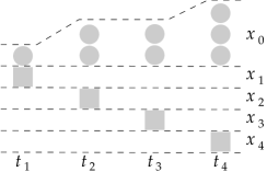
Figure 1. A list of terms that does not satisfy Buchberger’s Criteria, but satisfies the Extended Criterion. Observe that $\gcd\left(t_{1},t_{4}\right)$ divides $t_{2}$ and $t_{3}$, and $\left\{\deg_{x_{0}}t_{i}\right\}_{i=1}^{4}$ is monotonic.

 

On the other hand, the list $T_{3}=\left(x_{0}x_{1},x_{0}^{2}x_{2},x_{0}^{3}x_{3},x_{0}^{2}x_{4}\right)$ does not satisfy (EC), because (EVar) is violated: $\left\{\deg_{x_{0}}t_{k}\right\}_{k=1}^{m}=\left(1,2,3,2\right)$ is not monotonic. This is illustrated by Figure 2.

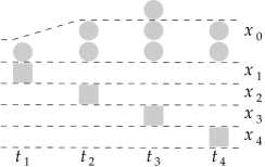
Figure 2. A list of terms that satisfy neither Buchberger’s Criteria nor the Extended Criterion. Observe that although $\gcd\left(t_{1},t_{4}\right)$ divides $t_{2}$ and $t_{3}$, $\left\{\deg_{x_{0}}t_{i}\right\}_{i=1}^{4}$ is not monotonic.

 

A permutation of $T_{3}$, $\left(x_{0}x_{1},x_{0}^{2}x_{2},x_{0}^{2}x_{4},x_{0}^{3}x_{3}\right)$, would satisfy (EC), but such permutations are not always possible if $t_{1}$ and $t_{m}$ share more than one variable; consider $\left(x_{1}yz,x_{2}y^{2}z,x_{3}yz^{2},x_{4}y^{3}z^{2},x_{5}yz\right)$.$\ \Diamond$

We can use the Extended Criterion to generalize Buchberger’s Characterization Theorem.

Main Theorem.

Let $G\in\mathcal{R}^{m}$. The following are equivalent.

• $G$ is a Gröbner basis with respect to $\prec$.

• For every $i,j$ such that $1\leq i<j\leq m$, one of the following holds:

  • $S_{\prec}\left({g_{i},g_{j}}\right)$ reduces to zero with respect to $G$.

  • $\mathrm{lt}_{\prec}\left(g_{i}\right)$ and $\mathrm{lt}_{\prec}\left(g_{j}\right)$ are relatively prime.

  • There exist $k_{1},\ldots,k_{n}$ such that $i=k_{1}$, $j=k_{n}$,
    each of the $\mathrm{lt}_{\prec}\left(g_{k_{\ell}}\right)$ divides $\mathrm{lcm}\left(\mathrm{lt}_{\prec}\left(g_{i}\right),\mathrm{lt}_{\prec}\left(g_{j}\right)\right)$, and
    each $S_{\prec}\left({g_{k_{\ell}},g_{k_{\ell+1}}}\right)$ reduces to zero with respect to $G$.

  • There exist $k_{1},\ldots,k_{n}$ such that $i=k_{1}$, $j=k_{n}$,
    the list of leading terms of $g_{k_{1}},\ldots,g_{k_{n}}$ satisfy EC, and
    each $S_{\prec}\left({g_{k_{\ell}},g_{k_{\ell+1}}}\right)$ reduces to zero with respect to $G^{\prime}=\left(g_{k_{1}},\ldots,g_{k_{n}}\right)$.$\ \Diamond$

It is essential that in (B3), the reductions to zero are with respect to $G^{\prime}$ and not to $G$. If we use $G$ instead of $G^{\prime}$, then we may not have a Gröbner basis; see Example 8. This also makes it a bad idea to try to combine (B3) and (B2) into one disjunction.

If the terms $t_{1}$ and $t_{m}$ are relatively prime, then $\left(t_{1},\ldots,t_{m}\right)$ satisfies (EDiv) and (EVar) easily. Hence, pairs of leading terms that satisfy Buchberger’s gcd Criterion also satisfy the Extended Criterion. However, it is not easy to condense (B1) and (B3) into one criterion, because (B3) requires that a chain of $S$-polynomials reduce to zero, while (B1) does not.

When $m=3$, EC is equivalent to the criterion of [13], which generalizes both of Buchberger’s Criteria. For $m>3$, this is not the case! Terms can satisfy Buchberger’s lcm Criterion without satisfying EC, and as in Example 6, terms can satisfy EC without satisfying Buchberger’s lcm Criterion.

The remainder of this section consists of examples:

• Example 7 provides a straightforward application of the Main Theorem;

• Example 8 shows an invalid application of the Main Theorem.

Example 7.

Let $G=\left(g_{1},g_{2},g_{3},g_{4}\right)$ where

$$g_{1} =4x_{0}x_{1}+2x_{0}x_{2}+3x_{0}x_{4}-8x_{1}-4x_{2}-6x_{4}$$

$$g_{2} =3x_{0}^{2}x_{2}+2x_{0}^{2}x_{4}-6x_{0}x_{2}-4x_{0}x_{4}$$

$$g_{3} =4x_{0}^{2}x_{3}+2x_{0}^{2}x_{4}-8x_{0}x_{3}-4x_{0}x_{4}$$

$$g_{4} =2x_{0}^{3}x_{4}-2x_{0}^{2}x_{3}-x_{0}^{2}x_{4}+4x_{0}x_{3}-6x_{0}x_{4}.$$

Let $\prec$ represent any term ordering such that $\mathrm{lt}_{\prec}\left(g_{1}\right)=x_{0}x_{1}$, $\mathrm{lt}_{\prec}\left(g_{2}\right)=x_{0}^{2}x_{2}$, $\mathrm{lt}_{\prec}\left(g_{3}\right)=x_{0}^{2}x_{3}$, and $\mathrm{lt}_{\prec}\left(g_{4}\right)=x_{0}^{3}x_{4}$. We pose this question: Is $G$ a Gröbner basis with respect to $\prec$?

Routine computation verifies that the pairs $\left(1,2\right)$, $\left(2,3\right)$, and $\left(3,4\right)$ satisfy (B0) of Theorem 3 and of the Main Theorem; that is, $S_{\prec}\left({g_{1},g_{2}}\right)$, $S_{\prec}\left({g_{2},g_{3}}\right)$, and $S_{\prec}\left({g_{3},g_{4}}\right)$ reduce to zero with respect to $G$. We can say something more: in the process of reducing them, we discover that for $i=1,2,3$ each $S_{\prec}\left({g_{i},g_{i+1}}\right)$ reduces to zero with respect to $\{g_{i},g_{i+1}\}$. This will prove important in a moment.

As for the remaining pairs, they do not satisfy (B1) or (B2) of either theorem, because no permutation of the leading terms $x_{0}x_{1}$, $x_{0}^{2}x_{2}$, $x_{0}^{2}x_{3}$, and $x_{0}^{3}x_{4}$ satisfies Buchberger’s criteria. Thus, Theorem 3 does not help us answer the question posed.

However, the Main Theorem does. Observe that

$$\left(\mathrm{lt}_{\prec}\left(g_{1}\right),\mathrm{lt}_{\prec}\left(g_{2}\right),\mathrm{lt}_{\prec}\left(g_{3}\right),\mathrm{lt}_{\prec}\left(g_{4}\right)\right)=T_{2}$$

where $T_{2}$ was defined in Example 7; the Extended Criterion applies to $T_{2}$. In addition, $S_{\prec}\left({g_{1},g_{2}}\right)$, $S_{\prec}\left({g_{2},g_{3}}\right)$, and $S_{\prec}\left({g_{3},g_{4}}\right)$ reduce to zero with respect to $G$. Hence $(1,4)$ satisfies (B3) of the Main Theorem with $G^{\prime}=G$.

We are not quite done: to decide whether $G$ is a Gröbner basis, we must resolve the pairs $(1,3)$ and $(2,4)$. The Main Theorem shows that these pairs also satisfy (B0).

• To show that $S_{\prec}\left({g_{1},g_{3}}\right)$ reduces to zero, we claim that $\{g_{1},g_{2},g_{3}\}$ is a Gröbner basis:

  • We know that the pairs $(1,2)$ and $(2,3)$ satisfy (B0) of the Main Theorem.

  • The Extended Criterion applies to $\left(\mathrm{lt}_{\prec}\left(g_{1}\right),\mathrm{lt}_{\prec}\left(g_{2}\right),\mathrm{lt}_{\prec}\left(g_{3}\right)\right)$.

  • Recalling that each $S_{\prec}\left({g_{i},g_{i+1}}\right)$ reduces to zero w.r.t. $\{g_{i},g_{i+1}\}$, we infer that $S_{\prec}\left({g_{1},g_{2}}\right)$ and $S_{\prec}\left({g_{2},g_{3}}\right)$ reduce to zero w.r.t. $G^{(1,2,3)}=\left(g_{1},g_{2},g_{3}\right)$. Thus the pair $(1,3)$ satisfies (B3) of the Main Theorem.

  • This implies that $G^{(1,2,3)}$ is a Gröbner basis, so $S_{\prec}\left({g_{1},g_{3}}\right)$ reduces to zero.

• To show that $S_{\prec}\left({g_{2},g_{4}}\right)$ reduces to zero, we claim that $\{g_{2},g_{3},g_{4}\}$ is a Gröbner basis:

  • We know that the pairs $(2,3)$ and $(3,4)$ satisfy (B0) of the Main Theorem.

  • The Extended Criterion applies to $\left(\mathrm{lt}_{\prec}\left(g_{2}\right),\mathrm{lt}_{\prec}\left(g_{3}\right),\mathrm{lt}_{\prec}\left(g_{4}\right)\right)$.

  • Recalling that each $S_{\prec}\left({g_{i},g_{i+1}}\right)$ reduces to zero w.r.t. $\{g_{i},g_{i+1}\}$, we infer that $S_{\prec}\left({g_{2},g_{3}}\right)$ and $S_{\prec}\left({g_{3},g_{4}}\right)$ reduce to zero w.r.t. $G^{(2,3,4)}=\left(g_{2},g_{3},g_{4}\right)$. Thus the pair $(2,4)$ satisfies (B3) of the Main Theorem.

  • This implies that $G^{(2,3,4)}$ is a Gröbner basis, so $S_{\prec}\left({g_{2},g_{4}}\right)$ reduces to zero.

Recall that $(1,4)$ satisfies (B3) of the Main Theorem with $G^{\prime}=G$. We now know that the other pairs satisfy (B0). It follows from the Main Theorem that $G$ is indeed a Gröbner basis with respect to $\prec$. We have answered the question posed by reducing only three of the six $S$-polynomials to zero.

To achieve this, we had to know not only that the $S$-polynomials reduced to zero, but also over which subsets of $G$ they were reduced! Had those subsets been different, the Extended Criterion probably would not apply, as Example 8 shows below. Conversely, it is conceivable that one could apply the Extended Criterion but not realize it, because one has verified that the $S$-polynomials in question reduce to zero with respect to a different subset of $G$ than the one needed.$\ \Diamond$

The following example illustrates why (B3) of the Main Theorem requires $G^{\prime}$ and not $G$.

Example 8.

Let $G=\left(g_{1},g_{2},g_{3},g_{4}\right)$ where

$$g_{1} =x^{2}y+z$$

$$g_{2} =xyz$$

$$g_{3} =xy^{2}$$

$$g_{4} =z^{2}.$$

Let $\prec$ be any ordering such that $x^{2}y\succ z$. Again we ask, Is $G$ a Gröbner basis with respect to $\prec$?

It is easy to verify that pairs $\left(1,2\right)$, $\left(1,4\right)$, $\left(2,3\right)$, $\left(2,4\right)$, and $\left(3,4\right)$ satisfy (B0) of the Main Theorem. The leading terms of $g_{1}$, $g_{2}$, and $g_{3}$ satisfy the Extended Criterion, so set $G^{\prime}=\left(g_{1},g_{2},g_{3}\right)$. A subquestion: Does (B3) of the Main Theorem imply that $G$ is a Gröbner basis? No, because the $S$-polynomials $S_{\prec}\left({g_{1},g_{2}}\right)$ and $S_{\prec}\left({g_{2},g_{3}}\right)$ reduce to zero with respect to $G$, but not with respect to $G^{\prime}$. In fact, $S_{\prec}\left({g_{1},g_{3}}\right)=yz$ does not reduce to zero with respect to $G$ even though all the other $S$-polynomials do! Thus $G$ is not a Gröbner basis with respect to $\prec$.$\ \Diamond$

3. Proof of the Main Theorem

Before diving into details, we pause a moment to describe the fundamental goal of the proof. A previous example will serve us well. The polynomials of Example 7 factor as follows:

$$g_{1} =\phantom{2x_{0}}\left(x_{0}-2\right)\left(4x_{1}+2x_{2}+3x_{4}\right)$$

$$g_{2} =\phantom{2}x_{0}\left(x_{0}-2\right)\left(3x_{2}+2x_{4}\right)$$

$$g_{3} =2x_{0}\left(x_{0}-2\right)\left(2x_{3}+x_{4}\right)$$

$$g_{4} =\phantom{2}x_{0}\left(x_{0}-2\right)\left(2x_{0}x_{4}+3x_{4}-2x_{3}\right).$$

Any pair of the polynomials has a common divisor whose cofactors have relatively prime leading terms: for example, the common divisor of $g_{1}$ and $g_{4}$ is $x_{0}-2$, and the leading terms of the cofactors are $x_{1}$ and $x_{0}^{2}x_{4}$, respectively. From (B1) of Theorem 3, we know that the system of cofactors of the gcd is a Gröbner basis. Generating a new system whose polynomials are multiples of the cofactors does not alter this, provided that for each pair the multiple of the cofactors is common.

The fundamental goal of the proof is to generalize this observation. Theorem 18 accomplishes this. Lemma 11 is a technical lemma that fills in a crucial step of Lemma 16, which in its turn is a technical lemma that fills in a crucial step of Theorem 18. Lemmas 12 and 14 are also technical lemmas that help clarify some linear algebra necessary for the proof of Lemma 11.

Although Lemmas 16 and 18 generalize similar lemmas in [13], the increased size of the list ($m>3$) required the development of the entirely new Lemma 11, as well as substantial changes to the proof of Lemma 16. In addition, Theorem 18 leads to the important consequence Corollary 17; this consequence went unremarked in the previous work, but will show itself useful in Section 4.

Besides a proof of the main theorem, this section develops several results that are interesting or useful in other contexts. Lemma 11, for example, took us completely by surprise. Lemma 16 generalizes a relationship between the gcd of two polynomials and their $S$-polynomial. Theorem 18 is similar to a well-known theorem regarding Buchberger’s lcm Criterion; it will prove useful in Section 4, whereas the Main Theorem does not.

We turn to the proof. We regularly make implicit use of Proposition 9 below. The proof is easy and well-known, so we do not repeat it here.

Proposition 9.

For all $f,g\in\mathcal{R}$ each of the following holds.

(A) If $f+g\neq 0$, then $\mathrm{lt}_{\prec}\left(f+g\right)\preceq\max_{\prec}\left(\mathrm{lt}_{\prec}\left(f\right),\mathrm{lt}_{\prec}\left(g\right)\right)$.

(B) $\mathrm{lt}_{\prec}\left(f\cdot g\right)=\mathrm{lt}_{\prec}\left(f\right)\cdot\mathrm{lt}_{\prec}\left(g\right)$.

(C) If $f/g$ is a polynomial, then $\mathrm{lt}_{\prec}\left(f/g\right)=\mathrm{lt}_{\prec}\left(f\right)/\mathrm{lt}_{\prec}\left(g\right)$.$\ \Diamond$

At this point we introduce the concept of an $S$-representation, which is essential to the proof.

Definition 10.

Let $p\in\mathcal{R}$, $t$ a term of $\mathcal{R}$, and $G\in\mathcal{R}^{m}$. We say that $\mathbf{h}\in\mathcal{R}^{m}$ is a $t$-representation of $p$ with respect to $G$ if $p=h_{1}g_{1}+\cdots+h_{m}g_{m}$ and for all $i$ such that $1\leq i\leq m$, we have $h_{i}=0$ or $\mathrm{lt}_{\prec}\left(h_{i}g_{i}\right)\preceq t$.

Furthermore, let $g_{i},g_{j}\in G$. If $t\prec\mathrm{lcm}\left(\mathrm{lt}_{\prec}\left(g_{i}\right),\mathrm{lt}_{\prec}\left(g_{j}\right)\right)$ and $\mathbf{h}$ is a $t$-representation of $S_{\prec}\left({g_{i},g_{j}}\right)$ with respect to $G$, then we say that $S_{\prec}\left({g_{i},g_{j}}\right)$ has an $S$-representation with respect to $G$, and that $\mathbf{h}$ is an $S$-representation of $S_{\prec}\left({g_{i},g_{j}}\right)$ with respect to $G$. We may omit “with respect to $G$” if it is clear from the context.$\ \Diamond$

The notion of $S$-representation is related, but not equivalent, to the notion of reduction to zero. We discuss this relationship near the end of the section, where it becomes important for the Main Theorem. For the time being, we content ourselves with exploring how the Extended Criterion can link a chain of $S$-representations.

To do that, we will need Lemma 11, which identifies a useful and interesting structure in a certain chain of $S$-representations.

Lemma 11.

Let $G\in\mathcal{R}^{m}$. Then (A) $\Longrightarrow$ (B) where

• $S_{\prec}\left({g_{1},g_{2}}\right)$, $S_{\prec}\left({g_{2},g_{3}}\right)$, …, and $S_{\prec}\left({g_{m-1},g_{m}}\right)$ all have $S$-representations with respect to $G$.

• There exist $P,Q\in\mathcal{R}$ such that $P\cdot g_{1}=Q\cdot g_{m}$ and

  • $\mathrm{lt}_{\prec}\left(P\right)=\sigma_{g_{1},g_{2}}\sigma_{g_{2},g_{3}}\cdots\sigma_{g_{m-1},g_{m}}$, and

  • $\mathrm{lt}_{\prec}\left(Q\right)=\sigma_{g_{2},g_{1}}\sigma_{g_{3},g_{2}}\cdots\sigma_{g_{m},g_{m-1}}$.$\ \Diamond$

The proof of Lemma 11 requires some non-trivial linear algebra, so we defer it to page 3. Lemmas 12 and 14 provide the necessary results. Lemma 12 describes a relationship between the elimination of variables in a linear system and the coefficients of those variables.

Lemma 12.

Let $n\in\mathbb{N^{+}}$. Consider the system of $n-1$ linear equations in $n$ variables

$$\mathcal{S}_{1}=\left\{\sum_{j=1}^{n}a_{i,j}x_{j}\right\}_{i=1}^{n-1}.$$

For $k=1,\ldots,n-2$ define the matrix

$$A_{k}=\left(\begin{array}[]{cccc}a_{1,1}&a_{1,2}&\cdots&a_{1,k}\\ a_{2,1}&a_{2,2}&\cdots&a_{2,k}\\ \vdots&&\ddots&\vdots\\ a_{k,1}&a_{k,2}&\cdots&a_{k,k}\end{array}\right).$$

If each $A_{k}$ has nonzero determinant, then for each $k=2,\ldots,n-1$ the system

$$\mathcal{S}_{k}=\left\{\sum_{j=i}^{n}b_{i,j}^{(k)}x_{j}=0\right\}_{i=k}^{n-1}$$

with

$$b_{i,j}^{(k)}=\left|\begin{array}[]{cc}A_{k-1}&\begin{array}[]{c}a_{1,j}\\ a_{2,j}\\ \vdots\\ a_{k-1,j}\end{array}\\ \begin{array}[]{cccc}a_{i,1}&a_{i,2}&\cdots&a_{i,k-1}\end{array}&a_{i,j}\end{array}\right|$$

is consistent.$\ \Diamond$

To prove Lemma 12, we use the following special case of Jacobi’s Theorem on determinants, whose proof we do not reproduce here [14, 19].

Theorem 13.

Let $A$ be an $n\times n$ matrix, $M$ a $2\times 2$ minor of $A$, $M^{\prime}$ the corresponding $2\times 2$ minor of the adjugate of $A$, and $M^{*}$ the $\left(n-2\right)\times\left(n-2\right)$ minor of $A$ that is complementary to $M$. Then

$$\det M^{\prime}=\det A\cdot\det M^{*}.\ \Diamond$$

We will use Theorem 13 by putting $M$ as the corners of the matrix, making $M^{*}$ the interior.

Proof of Lemma 12.

We proceed by induction on $k$. For the inductive base $k=2$, eliminate $x_{1}$ from equations $i=2,\ldots,n-1$ in $\mathcal{S}_{1}$ by subtracting the product of the first equation and $a_{i,1}$ from the product of the second equation and $a_{1,1}$. It is routine to verify that for $i=2,\ldots,n-1$ and $j=2,\ldots,n$ we have

$$b_{i,j}^{(k)}=\left|\begin{array}[]{cc}a_{1,1}&a_{1,j}\\ a_{i,1}&a_{i,j}\end{array}\right|.$$

Now assume the assertion is true for all $\ell$ where $1\leq\ell<k$. In system $\mathcal{S}_{k-1}$ use equation $k-1$ to eliminate the variable $x_{k-1}$ from equations $k$, …, $n-1$. We obtain a new system of equations

$$\mathcal{S}_{k}=\left\{\sum_{j=i}^{n}\beta_{i,j}x_{j}=0\right\}_{i=k}^{n-1}$$

where for each $i,j,k$ we have

$$\beta_{i,j} =\left|\begin{array}[]{cc}b_{k-1,k-1}^{(k-1)}&b_{k-1,j}^{(k-1)}\\ \\ b_{i,k-1}^{(k-1)}&b_{i,j}^{(k-1)}\end{array}\right|$$

$$=\left|\begin{array}[]{cc}A_{k-2}&\begin{array}[]{c}a_{1,k-1}\\ \vdots\\ a_{k-2,k-1}\end{array}\\ a_{k-1,1}\quad\cdots\quad a_{k-1,k-2}&a_{k-1,k-1}\end{array}\right|\left|\begin{array}[]{cc}A_{k-2}&\begin{array}[]{c}a_{1,j}\\ \vdots\\ a_{k-2,j}\end{array}\\ a_{i,1}\quad\cdots\quad a_{i,k-2}&a_{i,j}\end{array}\right|$$

$$\quad-\left|\begin{array}[]{cc}A_{k-2}&\begin{array}[]{c}a_{1,k-1}\\ \vdots\\ a_{k-2,k-1}\end{array}\\ a_{i,1}\quad\cdots\quad a_{i,k-2}&a_{i,k-1}\end{array}\right|\left|\begin{array}[]{cc}A_{k-2}&\begin{array}[]{c}a_{1,j}\\ \vdots\\ a_{k-2,j}\end{array}\\ a_{k-1,1}\quad\cdots\quad a_{k-1,k-2}&a_{k-1,j}\end{array}\right|.$$

Perform the following row and column swaps:

• in $b_{k-1,k-1}^{(k-1)}$, move the bottom row to the top, and the rightmost row to the leftmost;

• in $b_{k-1,j}^{(k-1)}$, do nothing;

• in $b_{i,k-1}^{(k-1)}$, move the rightmost row to the leftmost; and

• in $b_{i,j}^{(k-1)}$, move the bottom row to the top.

Denote the resulting matrices by $B_{1}$, $B_{2}$, $B_{3}$, and $B_{4}$; the negatives introduced by the row and column swap cancel, so that $\beta_{i,j}=B_{1}B_{2}-B_{3}B_{4}$.

Let

$$C=\left|\begin{array}[]{ccccc}a_{k-1,k-1}&a_{k-1,1}&\cdots&a_{k-1,k-2}&a_{k-1,j}\\ a_{1,k-1}&&&&a_{1,j}\\ \vdots&&A_{k-2}&&\vdots\\ a_{k-2,k-1}&&&&a_{k-2,j}\\ a_{i,k-1}&a_{i,1}&\cdots&a_{i,k-2}&a_{i,j}\end{array}\right|.$$

Theorem 13 with

$$M=\left(\begin{array}[]{cc}a_{k-1,k-1}&a_{k-1,j}\\ a_{i,k-1}&a_{i,j}\end{array}\right)\mbox{ and }M^{*}=A_{k-2}$$

implies that

$$\beta_{i,j}=\left|C\right|\cdot\left|A_{k-2}\right|.$$

Move the top row of $C$ to the next-to-last row, and the leftmost row of $C$ to the next-to-last column; the negatives introduced by the row and column swaps cancel, so that

$$\beta_{i,j}=\left|\begin{array}[]{cccc}&&&a_{1,j}\\ &A_{k-1}&&\vdots\\ &&&a_{k-1,j}\\ a_{i,1}&\cdots&a_{i,k-1}&a_{i,j}\end{array}\right|\left|A_{k-2}\right|.$$

From the assumption that $A_{k-2}$ is nonzero, we can divide each equation of $\mathcal{S}_{k}$ by $A_{k-2}$, obtaining the desired linear system. ∎

From this point on, the presence of several $S$-representations requires a notation that will allow us to distinguish them.

Notation.

Let $G\in\mathcal{R}^{m}$. Let $i,j\in\left\{1,\ldots,m-1\right\}$ be distinct. We write

$$\mathbf{h}^{\left(i,j\right)}=\left(h_{1}^{\left(i,j\right)},h_{2}^{\left(i,j\right)},\ldots,h_{m}^{\left(i,j\right)}\right)$$

for an $S$-representation of $S_{\prec}\left({g_{i},g_{j}}\right)$ with respect to $G$. In addition, when $i<j$ we write

$$Z_{i,j} =-\mathrm{lc}_{\prec}\left(g_{j}\right)\sigma_{g_{i},g_{j}}+h_{i}^{\left(i,j\right)}$$

$$Z_{j,i} =\mathrm{lc}_{\prec}\left(g_{i}\right)\sigma_{g_{j},g_{i}}+h_{j}^{\left(i,j\right)}.$$

Note that $\mathrm{lt}_{\prec}\left(Z_{i,j}\right)=\sigma_{g_{i},g_{j}}$ and $\mathrm{lt}_{\prec}\left(Z_{j,i}\right)=\sigma_{g_{j},g_{i}}$.$\ \Diamond$

In the proof of Lemma 11 we will simplify a linear system of the form shown in Lemma 12. To perform this simplification, we must ascertain that the matrices $A_{k}$ in that context have nonzero determinant.

Lemma 14.

Let $G\in\mathcal{R}^{m}$. Then (A) $\Longrightarrow$ (B) where

• $S_{\prec}\left({g_{1},g_{2}}\right)$, $S_{\prec}\left({g_{2},g_{3}}\right)$, …, and $S_{\prec}\left({g_{m-1},g_{m}}\right)$ all have $S$-representations with respect to $G$.

• For each $k=2,\ldots,m-1$ the $k\times k$ matrix

  $$A_{k}=\left(\begin{array}[]{ccccc}Z_{2,1}&h_{3}^{(1,2)}&h_{4}^{(1,2)}&\cdots&h_{k+1}^{(1,2)}\\ Z_{2,3}&Z_{3,2}&h_{4}^{(2,3)}&\cdots&h_{k+1}^{(2,3)}\\ h_{2}^{(3,4)}&\ddots&\ddots&&h_{k+1}^{(3,4)}\\ \vdots&&\ddots&\ddots&\vdots\\ h_{2}^{(k,k+1)}&\cdots&h_{k-2}^{(k,k+1)}&Z_{k,k+1}&Z_{k+1,k}\end{array}\right)$$

  has nonzero determinant; indeed $\mathrm{lt}_{\prec}\left(\det A_{k}\right)=\sigma_{2,1}\sigma_{3,2}\cdots\sigma_{k+1,k}$.$\ \Diamond$

The proof of Lemma 14 is tricky, so we present a simple but nontrivial example to illustrate the strategy.

Example 15.

Suppose $m>3$ and the system $G\in\mathcal{R}^{m}$ satisfies (A) of Lemma 14. We show that (B) is satisfied for $k=3$. A determinant is a sum of elementary products; since

$$A_{3}=\left(\begin{array}[]{ccc}Z_{2,1}&h_{3}^{(1,2)}&h_{4}^{(1,2)}\\ Z_{2,3}&Z_{3,2}&h_{4}^{(2,3)}\\ h_{2}^{(3,4)}&Z_{3,4}&Z_{4,3}\end{array}\right)$$

and the leading term of $Z_{2,1}Z_{3,2}Z_{4,3}$ is $\tau=\sigma_{2,1}\sigma_{3,2}\sigma_{4,3}$, the leading term of at least one elementary product of $\det A_{3}$ has the desired form.

We claim that the leading term of every other elementary product of $\det A_{3}$ is smaller than $\tau$. We proceed by way of contradiction. Assume that some other term in the elementary product has a leading term greater than or equal to $\tau$. Consider the leading terms of the other five polynomials, denoting $\mathrm{lcm}\left(\mathrm{lt}_{\prec}\left(g_{i}\right),\mathrm{lt}_{\prec}\left(g_{j}\right)\right)$ by $L_{i,j}$ and $\mathrm{lt}_{\prec}\left(g_{i}\right)$ by $t_{i}$.

• Suppose that $\tau\preceq\mathrm{lt}_{\prec}\left(h_{3}^{(1,2)}\cdot h_{4}^{(2,3)}\cdot h_{2}^{(3,4)}\right)$. Multiply both sides of the inequality by $t_{2}t_{3}t_{4}$ to obtain

  $$L_{1,2}L_{2,3}L_{3,4}\preceq\left[t_{3}\cdot\mathrm{lt}_{\prec}\left(h_{3}^{(1,2)}\right)\right]\left[t_{4}\cdot\mathrm{lt}_{\prec}\left(h_{4}^{(2,3)}\right)\right]\left[t_{2}\cdot\mathrm{lt}_{\prec}\left(h_{2}^{(3,4)}\right)\right],$$

  which contradicts the definition of an $S$-representation.

• Suppose that $\tau\preceq\mathrm{lt}_{\prec}\left(h_{4}^{(1,2)}\cdot Z_{2,3}\cdot Z_{3,4}\right)$. Multiply both sides of the inequality by $t_{2}t_{3}t_{4}$ to obtain

  $$L_{1,2}L_{2,3}L_{3,4}\preceq\left[t_{4}\cdot\mathrm{lt}_{\prec}\left(h_{4}^{(1,2)}\right)\right]\cdot L_{2,3}\cdot L_{3,4},$$

  and divide both sides by the common lcm’s to obtain

  $$L_{1,2}\preceq t_{4}\cdot\mathrm{lt}_{\prec}\left(h_{4}^{(1,2)}\right),$$

  which contradicts the definition of an $S$-representation.

• Suppose that $\tau\preceq\mathrm{lt}_{\prec}\left(h_{2}^{(3,4)}\cdot Z_{3,2}\cdot h_{4}^{(1,2)}\right)$. Multiply both sides of the inequality by $t_{2}t_{3}t_{4}$ to obtain

  $$L_{1,2}L_{2,3}L_{3,4}\preceq\left[t_{2}\cdot\mathrm{lt}_{\prec}\left(h_{2}^{(3,4)}\right)\right]\cdot L_{2,3}\cdot\left[t_{4}\cdot\mathrm{lt}_{\prec}\left(h_{4}^{(1,2)}\right)\right],$$

  and divide both sides by the common lcm to obtain

  $$L_{1,2}L_{3,4}\preceq\left[t_{2}\cdot\mathrm{lt}_{\prec}\left(h_{2}^{(3,4)}\right)\right]\left[t_{4}\cdot\mathrm{lt}_{\prec}\left(h_{4}^{(1,2)}\right)\right],$$

  which contradicts the definition of an $S$-representation.

• Suppose that $\tau\preceq\mathrm{lt}_{\prec}\left(Z_{(3,4)}\cdot h_{4}^{(2,3)}\cdot Z_{2,1}\right)$. Multiply both sides of the inequality by $t_{2}t_{3}t_{4}$ to obtain

  $$L_{1,2}L_{2,3}L_{3,4}\preceq L_{3,4}\cdot\left[t_{4}\cdot\mathrm{lt}_{\prec}\left(h_{4}^{(2,3)}\right)\right]\cdot L_{1,2},$$

  and divide both sides by the common lcm’s to obtain

  $$L_{2,3}\preceq t_{4}\cdot\mathrm{lt}_{\prec}\left(h_{4}^{(2,3)}\right),$$

  which contradicts the definition of an $S$-representation.

• Suppose that $\tau\preceq\mathrm{lt}_{\prec}\left(Z_{4,3}\cdot Z_{2,3}\cdot h_{3}^{(1,2)}\right)$. Multiply both sides of the inequality by $t_{2}t_{3}t_{4}$ to obtain

  $$L_{1,2}L_{2,3}L_{3,4}\preceq L_{3,4}\cdot L_{2,3}\cdot\left[t_{3}\cdot\mathrm{lt}_{\prec}\left(h_{3}^{(1,2)}\right)\right],$$

  and divide both sides by the common lcm’s to obtain

  $$L_{1,2}\preceq t_{3}\cdot\mathrm{lt}_{\prec}\left(h_{3}^{(1,2)}\right),$$

  which contradicts the definition of an $S$-representation.$\ \Diamond$

The proof of Lemma 14 follows this strategy. It is clear from the main diagonal of each $A_{k}$ that the leading term $t$ of one elementary product of the determinant of $A_{k}$ has the desired form; assume by way of contradiction that the leading term of another elementary product is greater than or equal to $t$; simplify the equivalent inequality by clearing the denominators and dividing the lcm’s; the resulting inequality will contradict the definition of an $S$-representation.

Proof of Lemma 14.

It is clear that $\det A_{k}$ is a polynomial, each of whose terms is an elementary product of the matrix. We can write any elementary product as $T=\prod_{i=1}^{k}B_{i}$ such that

• each $B_{i}$ is an element of row $i$; and

• if $i\neq j$ then $B_{i}$ and $B_{j}$ are elements of different columns.

As noted above, the main diagonal $A_{k}$ produces an elementary product whose leading term has the desired form; we claim that every other elementary product has a smaller leading term.

We proceed by way of contradiction. Assume that some elementary product $T$ besides the main diagonal satisfies

(1) $$\prod_{i=1}^{k}\sigma_{i+1,i}\preceq\mathrm{lt}_{\prec}\left(T\right).$$

Partition the set of factors of $T$ into three sets:

• $\mathcal{D}$, containing those factors which are on the main diagonal, which have the form $Z_{i+1,i}$ for some $i=1,\ldots,k$;

• $\mathcal{L}$, containing those factors which are immediately below the main diagonal, which have the form $Z_{i,i+1}$ for some $i=2,\ldots,k$; and

• $\mathcal{O}$, containing the other factors, which have the form $h_{i}^{(j,j+1)}$ for appropriate $i,j$.

Since $T$ is not the product of the main diagonal, the uniqueness of row and column representatives among the factors of $T$ implies that $\mathcal{O}$ is guaranteed to be nonempty.

Denote $\mathrm{lcm}\left(\mathrm{lt}_{\prec}\left(g_{i}\right),\mathrm{lt}_{\prec}\left(g_{j}\right)\right)$ by $L_{i,j}$ and $\mathrm{lt}_{\prec}\left(g_{i}\right)$ by $t_{i}$. Multiply both sides of (1) by $\prod_{\ell=2}^{k+1}t_{\ell}$. This results in the equation

$$\prod_{i=1}^{k}t_{i+1}\cdot\sigma_{i+1,i}\preceq\prod_{\ell=2}^{k+1}t_{\ell}\cdot\prod_{Z_{i+1,i}\in\mathcal{D}}\sigma_{i+1,i}\cdot\prod_{Z_{i,i+1}\in\mathcal{L}}\sigma_{i,i+1}\cdot\prod_{h_{i}^{(j,j+1)}\in\mathcal{O}}h_{i}^{(j,j+1)}.$$

Simplify the left hand side to obtain

(2) $$\prod_{i=1}^{k}L_{i,i+1}\preceq\prod_{\ell=2}^{k+1}t_{\ell}\cdot\prod_{Z_{i+1,i}\in\mathcal{D}}\sigma_{i+1,i}\cdot\prod_{Z_{i,i+1}\in\mathcal{L}}\sigma_{i,i+1}\cdot\prod_{h_{i}^{(j,j+1)}\in\mathcal{O}}h_{i}^{(j,j+1)}.$$

Rearrange the right hand side of (2) by pairing each $t_{\ell}$ with the corresponding factor taken from column $\ell-1$. The uniqueness of column representatives among the factors of an elementary product of a matrix guarantees a one-to-one pairing. If $t_{\ell}$ is paired with an element of

• $\mathcal{D}$, it is paired with $Z_{\ell,\ell-1}$, and the product simplifies to $L_{\ell-1,\ell}$;

• $\mathcal{L}$, it is paired with $Z_{\ell,\ell+1}$, and the product simplifies to $L_{\ell,\ell+1}$;

• if $t_{\ell}$ is paired with an element of $\mathcal{O}$, it is paired with $h_{\ell}^{(j,j+1)}$ for appropriate $j$.

In addition, the uniqueness of row representatives among the factors of an elementary product implies that for each $i$, at most one pairing simplifies to $L_{i,i+1}$. Thus, if we simplify the right hand side of (2) we have

$$\prod_{i=1}^{k}L_{i,i+1}\preceq\prod_{h_{i}^{(j,j+1)}\not\in\mathcal{O}}L_{i,i+1}\cdot\prod_{h_{i}^{(j,j+1)}\in\mathcal{O}}t_{i}h_{i}^{(j,j+1)}.$$

Divide both sides by $\prod_{h_{i}\not\in\mathcal{O}}L_{i,i+1}$ and we have

$$\prod_{h_{i}^{(j,j+1)}\in\mathcal{O}}L_{i,i+1}\preceq\prod_{h_{i}^{(j,j+1)}\in\mathcal{O}}t_{i}h_{i}^{(j,j+1)}.$$

Recall that $\mathcal{O}$ was guaranteed to be nonempty, so these products are greater than 1. This contradicts the definition of an $S$-representation.

We have shown that the leading term of the elementary product of $\det A_{k}$ formed on the main diagonal is $\prod_{i=1}^{k}\sigma_{i+1,i}$, while the leading terms of the remaining elementary products are strictly smaller. The sum of the elementary products thus derives its leading term from the main diagonal, whose leading term is the form described by (B). ∎

Finally we turn to the proof of Lemma 11.

Proof of Lemma 11.

Assume (A). We must show (B).

For each $i=1,\ldots,m-1$ fix $\mathbf{h}^{\left(i,i+1\right)}$, an $S$-representation of $S_{\prec}\left({g_{i},g_{i+1}}\right)$. We have the system of $m-1$ equations

$$\begin{array}[]{rlllll}Z_{1,2}g_{1}&+Z_{2,1}g_{2}&+h_{3}^{\left(1,2\right)}g_{3}&+\cdots&+h_{m}^{\left(1,2\right)}g_{m}&=0\\ &&&&&\vdots\\ h_{1}^{\left(m-1,m\right)}g_{1}&+\cdots&+h_{m-2}^{\left(m-1,m\right)}g_{m-2}&+Z_{m-1,m}g_{m-1}&+Z_{m,m-1}g_{m}&=0.\end{array}$$

Eliminate $g_{2}$, …, $g_{m-1}$ from the system. By Lemmas 12 and 14 (with $x_{i}=g_{i+1}$ for $i=1,\ldots,m-2$) we obtain $g_{1}P=g_{m}Q$ where

$$P=\left|\begin{array}[]{cccccc}Z_{1,2}&Z_{2,1}&h_{3}^{\left(1,2\right)}&\cdots&h_{m-2}^{\left(1,2\right)}&h_{m-1}^{\left(1,2\right)}\\ h_{1}^{\left(2,3\right)}&Z_{2,3}&Z_{3,2}&\ddots&h_{m-2}^{\left(2,3\right)}&h_{m-1}^{\left(2,3\right)}\\ \vdots&&\ddots\\ h_{1}^{\left(m-1,m\right)}&h_{2}^{\left(m-1,m\right)}&h_{3}^{\left(m-1,m\right)}&&h_{m-2}^{\left(m-1,m\right)}&Z_{m-1,m}\end{array}\right|$$

and

$$Q=\left|\begin{array}[]{cccccc}Z_{2,1}&h_{3}^{\left(1,2\right)}&\cdots&h_{m-2}^{\left(1,2\right)}&h_{m-1}^{\left(1,2\right)}&h_{m}^{\left(1,2\right)}\\ &\ddots&&&\ddots&\vdots\\ h_{2}^{\left(m-2,m-1\right)}&h_{3}^{\left(m-2,m-1\right)}&\ddots&Z_{m-2,m-1}&Z_{m-1,m-2}&h_{m}^{\left(m-2,m-1\right)}\\ h_{2}^{\left(m-1,m\right)}&h_{3}^{\left(m-1,m\right)}&\cdots&h_{m-2}^{\left(m-1,m\right)}&Z_{m-1,m}&Z_{m,m-1}\end{array}\right|.$$

To show that $\mathrm{lt}_{\prec}\left(P\right)$ and $\mathrm{lt}_{\prec}\left(Q\right)$ have the form specified by the lemma, apply an argument similar to the one used to prove Lemma 14. ∎

Gröbner basis theory generalizes many algorithms for univariate polynomials to systems of multivariate polynomials; one oft-cited example is how Buchberger’s algorithm to compute a Gröbner basis can be viewed as a generalization of the Euclidean algorithm to compute the gcd. We likewise expect relationships to exist between the $S$-polynomials and the gcd’s of polynomials.

Moreover, the construction of $S$-polynomials relies on the computation of

$$\sigma_{g_{i},g_{j}}=\frac{\mathrm{lcm}\left(\mathrm{lt}_{\prec}\left(g_{i}\right),\mathrm{lt}_{\prec}\left(g_{j}\right)\right)}{\mathrm{lt}_{\prec}\left(g_{i}\right)}$$

which can be rewritten as

$$\sigma_{g_{i},g_{j}}=\frac{\mathrm{lt}_{\prec}\left(g_{j}\right)}{\gcd\left(\mathrm{lt}_{\prec}\left(g_{i}\right),\mathrm{lt}_{\prec}\left(g_{j}\right)\right)}.$$

Based on this, one might expect the existence of criteria on $S$-polynomials that relate the gcd of two polynomials with the gcd of their leading terms.

One such criterion exists for two polynomials: if $G=\{g_{1},g_{2}\}$ is a Gröbner basis, then the $S$-polynomial of $g_{1}$ and $g_{2}$ reduces to zero, and in addition $g_{1}=f_{1}p$ and $g_{2}=f_{2}p$ where $p=\gcd\left(g_{1},g_{2}\right)$ and the leading terms of $f_{1}$ and $f_{2}$ are relatively prime [1]. In this case, we infer a surprising fact. Observe that

$$\mathrm{lt}_{\prec}\left(\gcd\left(g_{1},g_{2}\right)\right) =\mathrm{lt}_{\prec}\left(\gcd\left(f_{1}p,f_{2}p\right)\right)$$

$$=\mathrm{lt}_{\prec}\left(\gcd\left(f_{1},f_{2}\right)\cdot p\right).$$

Since $p$ is the gcd of $g_{1}$ and $g_{2}$, we know that $f_{1}$ and $f_{2}$ must be relatively prime, so

$$\mathrm{lt}_{\prec}\left(\gcd\left(g_{1},g_{2}\right)\right) =\mathrm{lt}_{\prec}\left(1\right)\cdot\mathrm{lt}_{\prec}\left(p\right)$$

$$=\gcd\left(\mathrm{lt}_{\prec}\left(f_{1}\right),\mathrm{lt}_{\prec}\left(f_{2}\right)\right)\cdot\mathrm{lt}_{\prec}\left(p\right)$$

$$=\gcd\left(\mathrm{lt}_{\prec}\left(f_{1}\right)\mathrm{lt}_{\prec}\left(p\right),\mathrm{lt}_{\prec}\left(f_{2}\right)\mathrm{lt}_{\prec}\left(p\right)\right)$$

$$=\gcd\left(\mathrm{lt}_{\prec}\left(g_{1}\right),\mathrm{lt}_{\prec}\left(g_{2}\right)\right).$$

Lemma 16 generalizes this observation in a way that does not require a Gröbner basis, but does require the Extended Criterion!

Lemma 16.

Let $G\in\mathcal{R}^{m}$, and suppose that the leading terms of $G$ satisfy the Extended Criterion. Then (A)$\Rightarrow$(B) where

• Each of $S_{\prec}\left({g_{1},g_{2}}\right)$, $S_{\prec}\left({g_{2},g_{3}}\right)$, …, $S_{\prec}\left({g_{m-1},g_{m}}\right)$ has an $S$-representation with respect to $G$.

• $\gcd\left(\mathrm{lt}_{\prec}\left(g_{1}\right),\mathrm{lt}_{\prec}\left(g_{m}\right)\right)=\mathrm{lt}_{\prec}\left(\gcd\left(g_{1},g_{m}\right)\right)$.$\ \Diamond$

Proof.

Assume (A). We must show (B). For the sake of convenience, denote $\mathrm{lt}_{\prec}\left(g_{i}\right)$ by $t_{i}$.

By Lemma 11, we have

$$g_{1}P=g_{m}Q$$

where

$$\mathrm{lt}_{\prec}\left(P\right)=\sigma_{g_{1},g_{2}}\sigma_{g_{2},g_{3}}\cdots\sigma_{g_{m-1},g_{m}}\quad\mbox{and}\quad\mathrm{lt}_{\prec}\left(Q\right)=\sigma_{g_{2},g_{1}}\sigma_{g_{3},g_{2}}\cdots\sigma_{g_{m},g_{m-1}}.$$

Let $p=\gcd\left(g_{1},g_{m}\right)$ and put $f_{1}=g_{1}/p$ and $f_{m}=g_{m}/p$. Then

(3) $$f_{1}P=f_{m}Q.$$

Since $f_{1},f_{m}$ are relatively prime, $f_{1}\mid Q$. Thus $\mathrm{lt}_{\prec}\left(f_{1}\right)$ divides $\mathrm{lt}_{\prec}\left(Q\right)$.

Observe that for any $i=1,\ldots,m-1$, we have

$$\sigma_{g_{i+1},g_{i}}=\frac{\mathrm{lcm}\left(t_{i},t_{i+1}\right)}{t_{i+1}}=\frac{t_{i}}{\gcd\left(t_{i},t_{i+1}\right)}.$$

Thus

$$\mathrm{lt}_{\prec}\left(f_{1}\right)\mid\frac{t_{1}t_{2}\cdots t_{m-1}}{\gcd\left(t_{1},t_{2}\right)\gcd\left(t_{2},t_{3}\right)\cdots\gcd\left(t_{m-1,m}\right)}.$$

Denote $\gcd\left(t_{i},t_{j}\right)$ by $d_{i,j}$. For all variables $x$, we have

$$\deg_{x}\mathrm{lt}_{\prec}\left(f_{1}\right) \leq\deg_{x}\frac{t_{1}\cdots t_{m-1}}{d_{1,2}d_{2,3}\cdots d_{m-1,m}}.$$

Recall that $f_{1}=g_{1}/p$. For all variables $x$, we have

$$\deg_{x}t_{1}-\deg_{x}\mathrm{lt}_{\prec}\left(p\right) \leq\sum_{1\leq i<m}\deg_{x}t_{i}-\sum_{1\leq i<m}\deg_{x}d_{i,i+1}$$

(4) $$\sum_{1\leq i<m}\deg_{x}d_{i,i+1} \leq\deg_{x}\mathrm{lt}_{\prec}\left(p\right)+\sum_{1<i<m}\deg_{x}t_{i}.$$

We claim that for all variables $x$, $\deg_{x}d_{1,m}\leq\deg_{x}\mathrm{lt}_{\prec}\left(p\right)$. Let $x$ be arbitrary, but fixed. If $\deg_{x}t_{1}=0$ or $\deg_{x}t_{m}=0$, the claim is trivially true. So assume $\deg_{x}t_{1}\neq 0$ and $\deg_{x}t_{m}\neq 0$. We consider two cases.

If $\deg_{x}t_{1}\leq\deg_{x}t_{m}$, then $\deg_{x}d_{1,m}=\deg_{x}t_{1}$. Recall that $t_{1}$, …, $t_{m}$ satisfy EC. Therefore $\deg_{x}t_{1}\leq\deg_{x}t_{2}\leq\cdots\leq\deg_{x}t_{m}$. Thus $\deg_{x}d_{i,i+1}=\deg_{x}t_{i}$ for all $i$ such that $1\leq i\leq m-1$. Apply this to (4) to obtain

$$\deg_{x}d_{1,m}=\deg_{x}t_{1}\leq\deg_{x}\mathrm{lt}_{\prec}\left(p\right).$$

If $\deg_{x}t_{1}\geq\deg_{x}t_{m}$, a similar argument gives $\deg_{x}d_{1,m}\leq\deg_{x}\mathrm{lt}_{\prec}\left(p\right)$.

Since $x$ is arbitrary, $d_{1,m}$ divides $\mathrm{lt}_{\prec}\left(p\right)$, or equivalently $\gcd\left(\mathrm{lt}_{\prec}\left(g_{1}\right),\mathrm{lt}_{\prec}\left(g_{m}\right)\right)$ divides $\mathrm{lt}_{\prec}\left(\gcd\left(g_{1},g_{m}\right)\right)$. That $\mathrm{lt}_{\prec}\left(\gcd\left(g_{1},g_{m}\right)\right)$ divides $\gcd\left(\mathrm{lt}_{\prec}\left(g_{1}\right),\mathrm{lt}_{\prec}\left(g_{m}\right)\right)$ is trivial. Hence $\mathrm{lt}_{\prec}\left(\gcd\left(g_{1},g_{m}\right)\right)=\gcd\left(\mathrm{lt}_{\prec}\left(g_{1}\right),\mathrm{lt}_{\prec}\left(g_{m}\right)\right)$. ∎

The following result will be useful both for the proof of the Main Theorem and for Section 4.

Corollary 17.

Let $G\in\mathcal{R}^{m}$, and suppose that the leading terms of $G$ satisfy the Extended Criterion. Then (A)$\Rightarrow$(B) where

• $S_{\prec}\left({g_{1},g_{2}}\right)$, $S_{\prec}\left({g_{2},g_{3}}\right)$, …, $S_{\prec}\left({g_{m-1},g_{m}}\right)$ all have $S$-representations with respect to $G$.

• If $p=\gcd\left(g_{1},g_{m}\right)$, then $\mathrm{lt}_{\prec}\left(g_{1}/p\right)$ and $\mathrm{lt}_{\prec}\left(g_{m}/p\right)$ are relatively prime.$\ \Diamond$

Proof.

Assume (A). Let $p=\gcd\left(g_{1},g_{m}\right)$, and denote $g_{1}/p$ and $g_{m}/p$ by $f_{1}$ and $f_{m}$, respectively. From Lemma 16, we know that

$$\gcd\left(\mathrm{lt}_{\prec}\left(g_{1}\right),\mathrm{lt}_{\prec}\left(g_{m}\right)\right)=\mathrm{lt}_{\prec}\left(p\right).$$

Thus for any variable $x$,

$$\deg_{x}\gcd\left(\mathrm{lt}_{\prec}\left(g_{1}\right),\mathrm{lt}_{\prec}\left(g_{m}\right)\right) =\deg_{x}\mathrm{lt}_{\prec}\left(g_{1}\right)-\deg_{x}\mathrm{lt}_{\prec}\left(f_{1}\right)$$

$$=\deg_{x}\mathrm{lt}_{\prec}\left(g_{m}\right)-\deg_{x}\mathrm{lt}_{\prec}\left(f_{m}\right).$$

Let $x$ be arbitrary, but fixed. If $\deg_{x}\mathrm{lt}_{\prec}\left(g_{1}\right)\leq\deg_{x}\mathrm{lt}_{\prec}\left(g_{m}\right)$, then

$$\deg_{x}\mathrm{lt}_{\prec}\left(g_{1}\right)=\deg_{x}\gcd\left(\mathrm{lt}_{\prec}\left(g_{1}\right),\mathrm{lt}_{\prec}\left(g_{m}\right)\right)=\deg_{x}\mathrm{lt}_{\prec}\left(g_{1}\right)-\deg_{x}\mathrm{lt}_{\prec}\left(f_{1}\right),$$

so $\deg_{x}\mathrm{lt}_{\prec}\left(f_{1}\right)=0$. Similar reasoning shows that if $\deg_{x}\mathrm{lt}_{\prec}\left(g_{1}\right)\geq\deg_{x}\mathrm{lt}_{\prec}\left(g_{m}\right)$, then $\deg_{x}\mathrm{lt}_{\prec}\left(f_{m}\right)=0$. It follows that $\mathrm{lt}_{\prec}\left(g_{1}/p\right)$ and $\mathrm{lt}_{\prec}\left(g_{m}/p\right)$ are relatively prime. ∎

Theorem 18 is the main tool used to prove the Main Theorem. Note that a similar statement holds for Buchberger’s lcm Criterion, although the chain needed for the lcm Criterion, unlike the chain for the Extended Criterion, does not need to use all the polynomials of $G$.

Theorem 18.

Let $G\in\mathcal{R}^{m}$, and suppose that the leading terms of $G$ satisfy the Extended Criterion. Then (A)$\Rightarrow$(B) where

• $S_{\prec}\left({g_{1},g_{2}}\right)$, $S_{\prec}\left({g_{2},g_{3}}\right)$, …, $S_{\prec}\left({g_{m-1},g_{m}}\right)$ all have $S$-representations with respect to $G$.

• $S_{\prec}\left({g_{1},g_{m}}\right)$ has an $S$-representation with respect to $G$.$\ \Diamond$

Proof.

Assume (A). We want to show (B). For the sake of convenience, denote $\mathrm{lt}_{\prec}\left(g_{i}\right)$ by $t_{i}$.

Recall that

(5) $$S_{\prec}\left({g_{1},g_{m}}\right)=\mathrm{lc}_{\prec}\left(g_{m}\right)\cdot\frac{\mathrm{lcm}\left(t_{1},t_{m}\right)}{t_{1}}\cdot g_{1}-\mathrm{lc}_{\prec}\left(g_{1}\right)\cdot\frac{\mathrm{lcm}\left(t_{1},t_{m}\right)}{t_{m}}\cdot g_{m}.$$

Let $p=\gcd\left(g_{1},g_{m}\right)$ where $\mathrm{lc}_{\prec}\left(p\right)=1$. Put $f_{1}=g_{1}/p$ and $f_{m}=g_{m}/p$. From Lemma 16, we know that $\gcd\left(\mathrm{lt}_{\prec}\left(g_{1}\right),\mathrm{lt}_{\prec}\left(g_{m}\right)\right)=\mathrm{lt}_{\prec}\left(\gcd\left(g_{1},g_{m}\right)\right)$. This and the facts $\mathrm{lc}_{\prec}\left(f_{1}\right)=\mathrm{lc}_{\prec}\left(g_{1}\right)$ and $\mathrm{lc}_{\prec}\left(f_{m}\right)=\mathrm{lc}_{\prec}\left(g_{m}\right)$ give

$$\mathrm{lc}_{\prec}\left(g_{1}\right)\cdot\frac{\mathrm{lcm}\left(t_{1},t_{m}\right)}{t_{m}} =\mathrm{lc}_{\prec}\left(g_{1}\right)\cdot\frac{t_{1}t_{m}}{t_{m}\gcd\left(t_{1},t_{m}\right)}=\mathrm{lc}_{\prec}\left(f_{1}\right)\cdot\mathrm{lt}_{\prec}\left(f_{1}\right).$$

and

$$\mathrm{lc}_{\prec}\left(g_{m}\right)\cdot\frac{\mathrm{lcm}\left(t_{1},t_{m}\right)}{t_{1}} =\mathrm{lc}_{\prec}\left(g_{m}\right)\cdot\frac{t_{1}t_{m}}{t_{1}\gcd\left(t_{1},t_{m}\right)}=\mathrm{lc}_{\prec}\left(f_{m}\right)\cdot\mathrm{lt}_{\prec}\left(f_{m}\right)$$

This allows us to rewrite (5) as

$$S_{\prec}\left({g_{1},g_{m}}\right) =\mathrm{lc}_{\prec}\left(f_{m}\right)\mathrm{lt}_{\prec}\left(f_{m}\right)\cdot g_{1}-\mathrm{lc}_{\prec}\left(f_{1}\right)\mathrm{lt}_{\prec}\left(f_{1}\right)\cdot g_{m}$$

$$=p\cdot S_{\prec}\left({f_{1},f_{m}}\right).$$

By Corollary 17, the leading terms of $f_{1}$ and $f_{m}$ are relatively prime; by Buchberger’s gcd Criterion, $S_{\prec}\left({f_{1},f_{m}}\right)$ has an $S$-representation $\mathbf{h}$. It follows that $\mathbf{h}p=\left(h_{1}p,\ldots,h_{m}p\right)$ is an $S$-representation of $S_{\prec}\left({g_{1},g_{m}}\right)$. ∎

Theorem 18 provides us with sufficient information to conclude that the Main Theorem is true. This may not be clear, because we have discussed only $S$-representations, and not reduction to zero. To show how the two come together, we need to recall two additional results. The first is the characterization of Gröbner bases due to Lazard [17].

Theorem 19 (Lazard’s Characterization).

Let $G\in\mathcal{R}^{m}$. The following are equivalent.

• $G$ is a Gröbner basis with respect to $\prec$.

• For every $i,j$ such that $1\leq i<j\leq m$, $S_{\prec}\left({g_{i},g_{j}}\right)$ has an $S$-representation with respect to $G$.$\ \Diamond$

It turns out that Buchberger’s characterization implies Lazard’s, thanks to the following Lemma [3]:

Lemma 20.

Let $G\in\mathcal{R}^{m}$ and let $i,j$ satisfy $1\leq i<j\leq m$. Then (A)$\Longrightarrow$(B) where

• $S_{\prec}\left({g_{i},g_{j}}\right)$ reduces to zero with respect to $G$.

• $S_{\prec}\left({g_{i},g_{j}}\right)$ has an $S$-representation with respect to $G$.$\ \Diamond$

However, the converse of Lemma 20 is known to be false, so the fact that Lazard’s characterization implies Buchberger’s is not obvious. It depends on the fact that in Lazard’s characterization, every pair $(i,j)$ has an $S$-representation for $S_{\prec}\left({g_{i},g_{j}}\right)$, whereas Lemma  20 deals only with one $S$-representation.

We can now show how Theorem 18 proves the Main Theorem.

Proof of Main Theorem.

That (A) implies (B) is trivial, so we assume (B) and show (A). To prove (A), we will employ Lazard’s Characterization.

From (B), every pair $\left(i,j\right)$ satisfies one of (B0)—(B3). Let $i,j$ be such that $1\leq i<j\leq m$. Clearly $S_{\prec}\left({g_{i},g_{j}}\right)$ has an $S$-representation:

• if $\left(i,j\right)$ satisfies (B0), then by Lemma 20;

• if $\left(i,j\right)$ satisfies (B1) or (B2), then by well-known results [3, 1, 10];

• if $\left(i,j\right)$ satisfies (B3), then by Theorem 18.

By Lazard’s Characterization (Theorem 19), $G$ is a Gröbner basis with respect to $\prec$. ∎

4. “Pham-like” systems

In this section, we describe a class of polynomial systems for which the Extended Criterion provides a dramatic reduction in the number of $S$-polynomial computations required for verification (Corollary 23).

A well-studied system of polynomials is the Pham system [9, Chapter 6, p. 147].

Definition 21 (Pham system).

Let $P\in\mathbb{F}\left[x_{1},x_{2},\ldots,x_{n}\right]^{n}$. We say that $P$ is a Pham system if $\mathrm{lt}_{\prec}\left(p_{i}\right)$ and $\mathrm{lt}_{\prec}\left(p_{j}\right)$ are relatively prime whenever $i\neq j$.$\ \Diamond$

Thanks to Theorem 3, one can verify that any Pham system is a Gröbner basis without checking any $S$-polynomials at all. Now we obfuscate matters somewhat through multiplication.

Definition 22 (Pham-like systems).

Suppose that $G=\left(g_{1},\ldots,g_{m}\right)$ has leading terms $\left(c_{1}d,\ldots,c_{m}d\right)$ where for all $i=1,\ldots,m$,

• $c_{i}$ and $d$ are relatively prime, and

• for all $j\neq i$, $c_{i}$ and $c_{j}$ are relatively prime.

We call such $G$ a Pham-like system.$\ \Diamond$

Consider the following question.

Is a Pham-like system a Gröbner basis?

The temptation may arise to answer in the affirmative, because the cofactors of the leading terms’ gcd are relatively prime, which through some manipulation might allow Buchberger’s gcd Criterion to apply. It does not. Numerous systems are not Gröbner bases even though this property is true; for example,

$$g_{1}=xy+y,\quad g_{2}=xz.$$

So deciding whether $G$ is a Gröbner basis requires us to check whether the $S$-polynomials reduce to zero. We would like to avoid checking all of them if possible.

To that end, we turn first to Buchberger’s Criteria, but

• none of the leading terms $c_{i}d$, $c_{j}d$ are relatively prime; and

• for any pair $c_{i}d$ and $c_{j}d$, no $c_{k}d$ divides their lcm.

If we were to rely only on Buchberger’s Criteria, we would have to reduce all $m\left(m-1\right)/2$ $S$-polynomials to zero to see that a Pham-like system is a Gröbner basis.

However, the Extended Criterion allows us to decide whether a Pham-like system is a Gröbner basis by checking at most $m-1$ $S$-polynomials, even though Buchberger’s Criteria provide no benefit.

Corollary 23.

Let $G\in\mathcal{R}^{m}$ be a Pham-like system. The following are equivalent:

(A) $G$ is a Gröbner basis with respect to $\prec$.

(B) The $S$-polynomials $S_{\prec}\left({g_{1},g_{2}}\right)$, $S_{\prec}\left({g_{2},g_{3}}\right)$, …, $S_{\prec}\left({g_{m-1},g_{m}}\right)$ reduce to zero with respect to $G$.$\ \Diamond$

Proof.

That (A) implies (B) is trivial, so we assume (B) and show (A). From (B), we know that $S_{\prec}\left({g_{1},g_{2}}\right)$, $S_{\prec}\left({g_{2},g_{3}}\right)$, …, and $S_{\prec}\left({g_{m-1},g_{m}}\right)$ reduce to zero with respect to $G$. It follows from Lemma 20 that they have $S$-representations with respect to $G$.

For the sake of convenience, denote $\mathrm{lt}_{\prec}\left(g_{i}\right)$ by $t_{i}$. Write $t_{i}=c_{i}d$ where $c_{i}$ and $d$ are as in Definition 22. Recall that $\gcd\left(c_{i},t_{j}\right)=1$ whenever $i\neq j$; inspection shows that the list of terms $\left(t_{1},t_{2},\ldots,t_{m}\right)$ satisfies the Extended Criterion. By Theorem 18, $S_{\prec}\left({g_{1},g_{m}}\right)$ has an $S$-representation with respect to $G$. Let $p_{1,m}=\gcd\left(g_{1},g_{m}\right)$ and choose $f_{1},f_{m}\in\mathcal{R}$ such that

• $g_{1}=f_{1}p_{1,m}$, and

• $g_{m}=f_{m}p_{1,m}$.

Recall Lemma 16 and the assumption that $c_{1}$ is relatively prime to $t_{m}$; then

$$d=\gcd\left(c_{1}d,c_{m}d\right)=\gcd\left(\mathrm{lt}_{\prec}\left(g_{1}\right),\mathrm{lt}_{\prec}\left(g_{m}\right)\right)=\mathrm{lt}_{\prec}\left(p_{1,m}\right).$$

Thus

$$c_{1}d=t_{1}=\mathrm{lt}_{\prec}\left(g_{1}\right)=\mathrm{lt}_{\prec}\left(f_{1}p_{1,m}\right)=\mathrm{lt}_{\prec}\left(f_{1}\right)\mathrm{lt}_{\prec}\left(p_{1,m}\right)=\mathrm{lt}_{\prec}\left(f_{1}\right)d,$$

whence $c_{1}=\mathrm{lt}_{\prec}\left(f_{1}\right)$. Similarly, $c_{m}=\mathrm{lt}_{\prec}\left(f_{m}\right)$.

Inspection shows that the list of terms $\left(t_{1},t_{m},t_{m-1},\ldots,t_{3},t_{2}\right)$ also satisfies the Extended Criterion. We now know that $S_{\prec}\left({g_{1},g_{m}}\right)$ has an $S$-representation with respect to $G$, so we can reason as before that there exist $\varphi_{1},\varphi_{2},p_{1,2}\in\mathcal{R}$ such that

• $g_{1}=\varphi_{1}p_{1,2}$,

• $g_{2}=\varphi_{2}p_{1,2}$,

• $p_{1,2}=\gcd\left(g_{1},g_{2}\right)$, and

• the leading terms of $\varphi_{1}$ and $\varphi_{2}$ are relatively prime.

As before, we obtain $d=\mathrm{lt}_{\prec}\left(p_{1,2}\right)$ and $c_{1}=\mathrm{lt}_{\prec}\left(\varphi_{1}\right)$. Thus $\mathrm{lt}_{\prec}\left(f_{1}\right)=\mathrm{lt}_{\prec}\left(\varphi_{1}\right)$. We claim that in fact $f_{1}=\varphi_{1}$. By way of contradiction, assume that $f_{1}$ and $\varphi_{1}$ are not equal. From $f_{1}p_{1,m}=\varphi_{1}p_{1,2}$ we conclude that $f_{1}$ has a common factor with $p_{1,2}$ or $\varphi_{1}$ has a common factor with $p_{1,m}$—but this contradicts the hypothesis that $c_{1}$ is relatively prime to $d$. Hence $f_{1}=\varphi_{1}$ and $p_{1,m}=p_{1,2}$. Write $p=p_{1,m}$, $g_{1}=f_{1}p$, $g_{2}=f_{2}p$, and $g_{m}=f_{m}p$.

Proceeding in like fashion, we can factor every $g_{i}$ as $g_{i}=f_{i}p$ such that $\mathrm{lt}_{\prec}\left(f_{i}\right)$ and $\mathrm{lt}_{\prec}\left(f_{j}\right)$ are relatively prime whenever $i\neq j$. By Theorem 3, $F=\left(f_{1},f_{2},\ldots,f_{m}\right)$ is a Gröbner basis with respect to $\prec$. Let $i,j$ be arbitrary, but fixed. Assume $1\leq i<j\leq m$. By Lazard’s Characterization, $S_{\prec}\left({f_{i},f_{j}}\right)$ has an $S$-repre-sentation $\mathbf{h}^{\left(i,j\right)}$. This implies that $S_{\prec}\left({g_{i},g_{j}}\right)$ has an $S$-representation $p\mathbf{h}^{\left(i,j\right)}=\left(ph_{1}^{\left(i,j\right)},\ldots,ph_{m}^{\left(i,j\right)}\right)$. Since $i$ and $j$ are arbitrary, by Lazard’s Characterization $G$ is a Gröbner basis with respect to $\prec$. ∎

5. Acknowledgment

The author would like to thank the anonymous referee whose comments greatly improved the quality of the paper.

References

[1]William Adams and Philippe Loustaunau, An
Introduction to Gröbner Bases, vol. 3 of Graduate studies in
mathematics (American Mathematical Society, Providence, R.I., 1994).
[2]Jörgen Backelin and Ralf Fröberg, ‘How we proved
that there are exactly 924 cyclic-7 roots.’
‘ISSAC ’91: Proceedings of the 1991 International
Symposium on Symbolic and Algebraic Computation,’ (ACM Press, New
York, NY, USA, 1991).
ISBN ISBN:0-89791-437-6 pp. 103–111, pp. 103–111.
[3]Thomas Becker, Volker Weispfenning and Hans Kredel,
Gröbner Bases: a Computational Approach to Commutative Algebra
(Springer-Verlag New York, Inc., New York, 1993).
[4]Bruno Buchberger, ‘Ein Algorithmus zum Auffinden der
Basiselemente des Restklassenringes nach einem nulldimensionalem
Polynomideal (an algorithm for finding the basis elements in the residue
class ring modulo a zero dimensional polynomial ideal).’
Ph.D. thesis, Mathematical Insitute, University of Innsbruck,
Austria, (1965).
English translation published in the Journal of Symbolic
Computation (2006) 475–511.
[5]Bruno Buchberger, ‘An algorithmic criterion for the
solvability of a system of algebraic equations.’
Aequationes Mathematicae 4 (1970) 374–383.
English translation published in Gröbner Bases and
Applications, London Mathematical Society Lecture Note Series
251 (1998).
[6]Bruno Buchberger, ‘A criterion for detecting unnecessary
reductions in the construction of Gröbner bases.’
‘Proceedings of the EUROSAM 79 Symposium on Symbolic and
Algebraic Manipulation, Marseille, June 26-28, 1979,’ (ed. E. W.
Ng) (Springer, Berlin - Heidelberg - New York, 1979), vol. 72 of
Lecture Notes in Computer Science pp. 3–21, pp. 3–21.
[7]Bruno Buchberger, ‘Gröbner-bases: An algorithmic method
in polynomial ideal theory.’
‘Multidimensional Systems Theory - Progress, Directions and
Open Problems in Multidimensional Systems,’ (ed. N. K. Bose)
(Reidel Publishing Company, Dotrecht – Boston – Lancaster, 1985) pp.
184–232, pp. 184–232.
[8]Massimo Caboara, Martin Kreuzer and Lorenzo
Robbiano, ‘Minimal sets of critical pairs.’
‘Proceedings of the First Congress of Mathematical Software,’
(eds B. Cohen, X. Gao and N. Takayama) (World
Scientific, 2002) pp. 390–404, pp. 390–404.
[9]Arjeh M. Cohen, Hans Cuypers and Hans Sterk (eds),
Some Tapas of Computer Algebra, vol. 4 of Algorithms and
Computation in Mathematics (Springer, Berlin, 1999).
[10]David Cox, John Little and Donal O’Shea,
Ideals, Varieties, and Algorithms (Springer-Verlag New York, Inc.,
New York, 1997), 2nd edn.
[11]David Cox, John Little and Donal O’Shea,
Using Algebraic Geometry (Springer-Verlag New York, Inc., New York,
1998).
[12]Rudiger Gebauer and Hans Möller, ‘On an
installation of Buchberger’s algorithm.’
Journal of Symbolic Computation 6 (1988) 275–286.
[13]Hoon Hong and John Perry, ‘Are Buchberger’s
criteria necessary for the chain condition?’
Journal of Symbolic Computation 42 (2007) 717–732.
[14]Carl Gustav Jacob Jacobi, ‘De binis quibuslibet functionibus
homogeneis secundi ordinis per substitutiones lineares in alias binas
transformandis, quae solis quadratis variabilium constant; una cum variis
theorematis de transformatione et determinatione integralium multiplicium.’
Journal für die reine und angewandte Mathematik 12
(1833) 1–69.
[15]Christoph Kollreider and Bruno Buchberger, ‘An
improved algorithmic construction of Gröbner-bases for polynomial
ideals.’
ACM SIGSAM Bulletin 12 (1978) 27–36.
[16]Martin Kreuzer and Lorenzo Robbiano, Computational
Commutative Algebra I (Springer-Verlag, Heidelberg, 2000).
[17]Daniel Lazard, ‘Gröbner bases, Gaussian elimination,
and and resolution of systems of algebraic equations.’
‘EUROCAL ’83, European Computer Algebra Conference,’ (ed.
J. A. van Hulzen) (Springer LNCS, 1983), vol. 162 pp. 146–156, pp.
146–156.
[18]Hans Möller, Ferdinando Mora and Carlo
Traverso, ‘Gröbner bases computation using syzygies.’
‘Proceedings of the 1992 International Symposium on Symbolic
and Algebraic Computation,’ (ed. P. S. Wang). Association for
Computing Machinery (ACM Press, 1992) pp. 320–328, pp. 320–328.
[19]Adrian Rice and Eve Torrence, “‘Shutting up like a
telescope”: Lewis Carroll’s “curious” condensation method for
evaluating determinants.’
The College Mathematics Journal 38 (2007) 85–95.