Three-dimensional Radiative Properties of Hot Accretion Flows onto the Galactic Centre Black Hole

Abstract

By solving radiative transfer equations, we examine three-dimensional radiative properties of a magnetohydrodynamic accretion flow model confronting with the observed spectrum of Sgr A*, in the vicinity of supermassive black hole at the Galactic centre. As a result, we find that the core of radio emission is larger than the size of the event horizon shadow and its peak location is shifted from the gravitational centre. We also find that the self-absorbed synchrotron emissions by the superposition of thermal electrons within a few tens of the Schwartzschild radius can account for low-frequency spectra below the critical frequency $\nu_{c}\approx 10^{12}$ Hz. Above the critical frequency, the synchrotron self-Compton emission by thermal electrons can account for variable emissions in recent near-infrared observations. In contrast to the previous study by Ohsuga et al. (2005), we found that the X-ray spectra by Bremsstrahlung emission of thermal electrons for the different mass accretion rates can be consistent with both the flaring state and the quiescent state of Sgr A* observed by Chandra.

1 Introduction

How the emission comes from accreting material in the Galactic centre (GC) is a fundamental question for understanding the nature of mass accretion processes feeding a supermassive black hole (SMBH). When mass accretion rate is much less than the critical value, $\dot{M}_{\rm crit}\equiv L_{\rm Edd}/c^{2}$ where $L_{\rm Edd}\approx 1.3\times 10^{38}\left(M_{\rm BH}/M_{\odot}\right){\rm erg\,s^{-1}}$ is the Eddington luminosity and $c$ is the speed of the light, the radiation loss of accreting gas is inefficient and thus most of the energy generated by turbulent viscosity is stored as thermal energy of the gas and is advected onto SMBH. Therefore, the accretion flow becomes hot and geometrically thick structure. This type of accretion flow is well known as an advection-dominated accretion flow (ADAF: Ichimaru 1977; Narayan & Yi 1994, 1995; Abramowicz et al. 1995) or a radiatively inefficient accretion flows (RIAF: Yuan et al 2003; see also Kato, Fukue, Mineshige 2008). The ADAF/RIAF model is quite successful in reproducing high-energy emission of low-luminous active galactic nuclei (AGN) and the GC source, which is Sgr A* as a compact radio source (Balick & Brown 1974; Bower et al. 2004; Shen et al. 2005; Doeleman et al. 2008). Actually, the stellar dynamics has revealed the mass of SMBH in the GC, $\approx 4\times 10^{6}M_{\odot}$ (e.g., Schödel et al. 2002; Ghez et al. 2003, 2008; Gillessen et al. 2009). It turned out that the low-luminous material at the GC is associated with Sgr A*, in which the luminosity is $L_{\rm SgrA*}\approx 10^{-8}L_{\rm Edd}$.

After the discovery of magneto-rotational instability (MRI: Balbus & Hawley 1991, 1998), which can drive magnetohydrodynamic (MHD) turbulence as a source of viscosity for accretion process, it seems that non-radiative MHD simulations of accretion flows have been accepted as a realistic model of ADAF/RIAF (Stone & Pringle 2001; Hawley & Krolik 2001). For example, many MHD studies based on numerical simulations have revealed a hot and geometrically thick accretion flows with a variety of complex motions (Matsumoto et al. 1999; Hawley 2000; Machida et al. 2000), outflows and jets (Igumenshchev et al. 2003; Proga & Begelman 2003; Kato et al. 2004), and oscillations (Kato 2004). The recent detection of variability in the X-ray and near-infrared (NIR) emissions at Sgr A* (Baganoff et al. 2001, 2003; Ghez et al. 2004) may be induced by such a multi-dimensional structure of the flow. Nonlocal nature of radiation process is essential for testing MHD models. Therefore, in order to clarify the structure and the time variability of accretion flows, undoubtedly full radiation transfer treatment of MHD accretion flows in three-dimension is indispensable.

The pioneering work for examining MHD model of accretion flows has been done by Ohsuga, Kato, Mineshige (2005: hereafter OKM05). OKM05 assumed the cylindrical distribution of electron temperature by adopting the balance equation between radiative cooling and heating via Coulomb collision, regardless of gas temperature in MHD model. They reconstructed for the first time the multi-band spectrum of MHD model which is consistent with the observed spectra in flaring state of Sgr A*. However, the spectra in quiescent state cannot be reconstructed simultaneously in the radio and X-ray bands. In the context of MHD model, this is the issue of what makes the difference between the flaring state and the quiescent state in Sgr A*. We expect that determination of the electron temperature is the key for understanding the occurrence of two distinct states.

Moscibrodzka, Proga, Czerny, and Siemiginowska (2007: hereafter MPCS07) present the spectral feature of axisymmetric MHD flows by Proga & Begelman (2003). In contrast to OKM05, they calculate the electron temperature distribution by solving the heating-cooling balance equation at each grid point at a given time in the simulation. Moreover, they take into account the advective energy transport and compressive heating in the balance equation. It turns out that the heating of electrons via Coulomb collision is not always a dominant term in the balance equation. Unfortunately, MPCS07 failed to reproduce the radio and X-ray spectra by emission from thermal electron. They conclude that a contribution of non-thermal electrons offers a much better representation of the spectral variability of Sgr A*.

One difficulty in theoretical studies of radiative feature of hot accretion flows is that radiative energy transfer plays a critical role for determining the electron temperature. For example, radiative heating/cooling via synchrotron emission/absorption and Compton processes may dominate compressional heating and collisional heating in the energy balance equation at the high electron temperature (Rees et al. 1982). This makes everything rather complicated than the case of MPCS07. Conversely, once we know the properties of two-temperature plasma in MHD accretion flows which can reconstruct a radiation spectrum using a few relevant parameters, we can then constrain the physics of heating mechanism.

In this study, we investigate radiative signatures of radiatively inefficient accretion flows in long-term 3-D global MHD simulations. Then, confronting with the observed spectra of Sgr A* in the flaring and quiescent states, we derive constraints for electron temperature that can concordant with the observations. We also discuss heating mechanism of electron in the magnetized accretion flows. In §2 we present our 3-D MHD model of accretion flows and describe method of radiation transfer calculation. We then present our results in §3. The final section is devoted to summary and discussion.

2 Numerical Models and Methods

2.1 Setup of simulations

A physical model we use in this study is based on 3-D resistive MHD calculations with pseudo-Newtonian potential (see Kato, Mineshige, Shibata 2004; Kato 2004 for more details). We pick last 40 snapshots of our calculations from $t=30,000\,r_{\rm s}/c$ to $32,000\,r_{\rm s}/c$ with $dt=50r_{\rm s}/c$ where $r_{\rm s}$ and $c$ are the Schwartzschild radius and the speed of light, respectively. Note the flow has evolved in more than 600 rotation periods at the innermost stable circular orbits (ISCO) where the Keplerian rotation period is about $50r_{\rm s}/c$. Therefore our MHD model is supposed to be in quasi-steady state. In our radiation transfer calculations, we use uniform meshes as $(N_{\rm x},N_{\rm y},N_{\rm z})=(100,100,100)$ in Cartesian coordinates in a simulation box $|x,y,z|\leq 100\,r_{\rm s}$.

2.2 MHD model

The quasi-steady MHD accretion discs have a hot, geometrically thick structure associated with sub-thermal magnetic field. Fig. 1 displays a spatial distribution of the density, the gas temperature, and the strength of magnetic field of our MHD model. The density is normalized by the initial maximum density $\rho_{0}$ and the strength of magnetic field is proportional to $\left(\rho/\rho_{0}\right)^{1/2}$ for the same black hole mass $M_{\rm BH}$. As we can notice, an MHD disc has non-axisymmetric structures (close to $m=1$ where $m$ is the azimuthal mode number) in density, gas temperature, and strength of magnetic field, simultaneously. Moreover, filamentary structures of cold and dense gas can be seen in left and middle panels. Note that gas temperature is relatively high at funnel region along the z-axis because the centrifugal barriers prevent the penetration of accreting material. In right panel, MHD turbulence induced by MRI and the differential rotation in the flow generate strong magnetic field regions within approximately $30r_{\rm s}$.

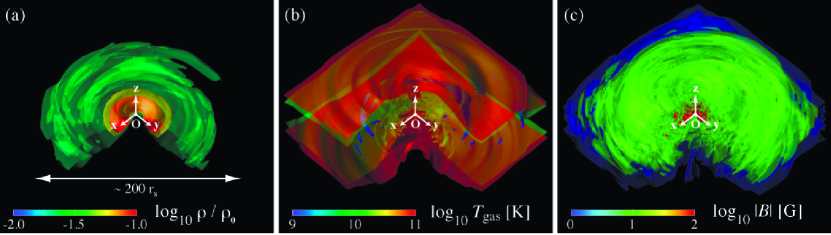
Figure 1: Perspective view of spatial distributions of density (left), gas temperature (middle), and strength of magnetic field (right) at $t=30000\,[r_{\rm s}/c]$. Normalized density is $\rho_{0}=8\times 10^{-15}\,{\rm[g\,cm^{-3}]}$.

2.3 Electron temperature

In our MHD model, it is assumed that the entire magnetic energy released in the diffusion region is thermalized instantly and therefore the production of non-thermal electrons accelerated by the magnetic reconnection is neglected for self-consistency. In the previous study OKM05, electron temperature is determined by the local thermal equilibrium between radiative cooling and electron heating via coulomb coupling in the cylindrical region. However, this assumption is invalid. Actually, in our preliminary radiation transfer calculation coupled with the energy balance equation, we found that the heating rate of coulomb coupling cannot afford the cooling rate of electrons in each computational cell. Therefore, the other heating mechanism of electrons, such as turbulent heating, must be taken into account for physical reasoning. Similar conclusions have been made by Sharma, Quataert, Hammett, & Stone (2007: hereafter SQHS07). For this reason, we introduce a new parameter, $f_{\rm ep}\equiv T_{\rm e}/T_{\rm p}$, the ratio of electron temperature and proton temperature so that electron temperature is determined with the gas temperature, $T_{\rm gas}$, by using $f_{\rm ep}$ in this study. We assume that $f_{\rm ep}$ is spatially uniform for simplicity. Thus electron temperature is obtained as:

$$T_{\rm e}=\min{\left(\frac{f_{\rm ep}}{1+f_{\rm ep}}T_{\rm gas},m_{\rm e}c^{2}/k_{\rm b}\right)}$$ (1)

where $T_{\rm gas}$ is the gas temperature which is derived by MHD simulation. We assume here that the electron temperature cannot exceed the temperature of rest mass energy of electron due to pair annihilation.

2.4 Parameters for radiation transfer calculation

There are only three model parameters, $\rho_{0}$, $f_{\rm ep}$, and $M_{\rm BH}$, in order to perform radiative transfer calculation in our study. The mass of SMBH in the GC is fixed at $M_{\rm BH}=3.6\times 10^{6}M_{\odot}$ (e.g., Schödel et al. 2002). The other model parameters we choose here are as follows: (a) $\rho_{0}=8\times 10^{-15}{\rm g\,cm^{-3}}$ and $f_{\rm ep}=0.25$, (b) $\rho_{0}=8\times 10^{-15}{\rm g\,cm^{-3}}$ and $f_{\rm ep}=1$, (c) $\rho_{0}=8\times 10^{-16}{\rm g\,cm^{-3}}$ and $f_{\rm ep}=0.25$, and (d) $\rho_{0}=8\times 10^{-16}{\rm g\,cm^{-3}}$ and $f_{\rm ep}=1$. Note that these parameters are derived by fitting the observed broadband spectra. Because the flow velocity is identical in all models, the larger density represent the more mass accretion rate $\dot{M}$. The relation between $\rho_{0}$ and $\dot{M}$ at ISCO can be described as follows:

$$\dot{M}\approx 2.5\times 10^{-7}\left({\rho_{0}\over 8\times 10^{-15}\,{\rm g\,cm^{-3}}}\right)M_{\odot}\,{\rm yr}^{-1}.$$ (2)

This relation indicates that mass accretion rate of our models is smaller than that for the quiescent X-ray emission measured with Chandra of $\dot{M}\sim 10^{-6}\,M_{\odot}\,{\rm yr}^{-1}$ at the Bondi radius (Baganoff et al. 2003), but is consistent with that estimated by the Faraday rotation in the millimeter band of $\dot{M}\sim 10^{-7}-10^{-8}\,M_{\odot}\,{\rm yr}^{-1}$ (Bower et al. 2003, 2005).

In radiation transfer calculation, we treat synchrotron emission/absorption, (inverse-)Compton scattering, and bremsstrahlung emission/absorption of the thermal electrons. Non-thermal electrons produced by collisions of protons via $\pi$-decay (Mahadevan et al. 1998) are not taken into account, because we focus only on the radiative properties of thermal electrons (Loeb & Waxman 2007).

2.5 Radiative transfer calculation

We solve the following radiation transfer equations with electron scattering by using Monte-Carlo method:

$$\mbox{\boldmath$n$}\cdot\nabla\mbox{\boldmath$I$}_{\nu}=\chi_{\nu}(\mbox{\boldmath$S$}_{\nu}-\mbox{\boldmath$I$}_{\nu})$$ (3)

where $\mbox{\boldmath$I$}_{\nu}(x,y,z,\theta,\phi)$ is the specific intensity at the position $(x,y,z)$ in the direction $(\theta,\phi)$ with the frequency $\nu$, whereas $\chi_{\nu}(x,y,z,\theta,\phi)=n_{\rm e}\sigma_{\nu}+\kappa_{\nu}$ is the extinction coefficient where $n_{\rm e}$, $\sigma_{\nu}$ and $\kappa_{\nu}$ is the electron number density, the scattering cross-section, and the absorption coefficient, respectively, and

$$\mbox{\boldmath$S$}_{\nu}={\varepsilon_{\nu}\over 4\pi\chi_{\nu}}+\oint\varphi(\nu,\mbox{\boldmath$n$};\nu^{\prime},\mbox{\boldmath$n$}^{\prime})\alpha_{\nu^{\prime}}\mbox{\boldmath$I$}_{\nu^{\prime}}(\mbox{\boldmath$n$}^{\prime})d\mbox{\boldmath$\Omega$}^{\prime}$$ (4)

is the source function where $\varepsilon_{\nu}$, $\alpha_{\nu}$, and $\varphi(\nu,\mbox{\boldmath$n$};\nu^{\prime}\mbox{\boldmath$n$}^{\prime})$ is the local emissivity, the scattering albedo, and the phase function, respectively. The coordinate system is shown in Fig. 2.

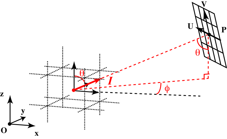
Figure 2: Geometry of radiation fields, $I$ in the coordinate space $(x,y,z,\theta,\phi)$ and coordinate screen $(u,v)$ for the ray-tracing calculation.

For generating photon packets, we randomly selected a position by using a local emissivity as follows:

$$\sum_{\rm i=1}^{\rm k-1}\varepsilon_{\nu}({\rm i})<R_{1}\sum_{\rm i=1}^{\rm Nmesh}\varepsilon_{\nu}({\rm i})<\sum_{\rm i=1}^{\rm k}\varepsilon_{\nu}({\rm i})$$ (5)

where $\varepsilon_{\nu}({\rm i})$ is the emissivity at the position index ${\rm i}$ and $R_{\rm 1}$ indicates a random number distributed uniformly in the interval $[0,1]$. In our study, all pseudo-random numbers $R_{\rm j}$ are generated by using a Mersenne Twister method (Matsumoto & Nishimura 1998). The direction of generated photon packets, $\mbox{\boldmath$n$}=(\sin{\theta}\cos{\theta},\sin{\theta}\sin{\phi},\cos{\theta})$, is also determined by using random numbers $R_{2}=(\cos{\theta}+1)/2$, $R_{3}=\phi/2\pi$. The frequency domain of photon packets is ranging from $10^{3}$ to $10^{25}$ Hz and is uniformally divided by 100 bins in logarithmic scale. In this study, $N_{\rm p}=10^{7}$ photon packets are generated in every frequency bin in order to acquire the statistically significant results.

In order to evaluate an escaping probability of an emerging photon packet, optical depth is computed by using a direct integration along the photon packet trajectory as follows:

$$\tau_{\nu}(l)=\int_{0}^{l}\left(n_{\rm e}\sigma_{\nu}+\kappa_{\nu}\right)ds,$$ (6)

where $l$ is a distance between the origin of the photon packet and the computational boundary along the trajectory. Here, we use the Klein-Nishina formula of scattering cross-section $\sigma_{\rm KN}$ for $\sigma_{\nu}$ (Rybicki & Lightman 1979) and the synchrotron, free-free, and bound-free self-absorption coefficient for $\kappa_{\nu}$ described by Kirchoff’s law assuming local thermal equilibrium (LTE) at every meshes,

$$\kappa_{\nu}=\frac{\varepsilon^{\rm sy}_{\nu}+\varepsilon^{\rm ff}_{\nu}+\varepsilon^{\rm bf}_{\nu}}{4\pi B_{\nu}}$$ (7)

where $\varepsilon^{\rm sy}_{\nu}$, $\varepsilon^{\rm ff}_{\nu}$, and $\varepsilon^{\rm bf}_{\nu}$ are synchrotron, free-free, and bound-free emissivity, respectively (Pacholczyk 1970; Stepney & Guilbert 1983), and $B_{\nu}$ is the Planck function. Accordingly, an escaping probability of the generated photon packet is written as:

$$w(l)=\exp{(-\tau_{\nu}(l))},$$ (8)

and the remaining photon packet $1-w(l)$ interacts with gas. Scattering position at the distance $l_{\rm s}$ from the original position is determined by using a random number as follows:

$$R_{4}=\left[1-w(l_{\rm s})\right]/\left[1-w(l)\right]$$ (9)

and the scattering albedo is given by:

$$\alpha_{\nu}=\frac{n_{\rm e}\sigma_{\nu}}{n_{\rm e}\sigma_{\nu}+\langle\kappa_{\nu}\rangle}$$ (10)

where $\langle\kappa_{\nu}\rangle$ is the mean absorption coefficient along the photon packet trajectory. To determine the phase function for the Compton scattering process, $\varphi(\nu,\mbox{\boldmath$n$};\nu^{\prime},\mbox{\boldmath$n$}^{\prime})$, we follow the method by Pozdnyakov et al. (1977). We repeat the same procedure for a scattered photon packet until either a photon is out of the computational box or $w(l)<\epsilon$ where $\epsilon=10^{-5}$ in this study. Note that photons can neither penetrate nor be generated at the region within 2 $r_{\rm s}$ in above calculation.

Finally, the computed radiation field is accumulated in the data array of $(N_{\rm x},N_{\rm y},N_{\rm z},N_{\theta},N_{\phi},N_{\nu})=(100,100,100,3,4,5)$ in order to generate synthetic images in a given frequency band and viewing angle. On the other hand, the computed spectrum of escaping photons in the fixed viewing angle is stored in the different data array.

3 Results

3.1 Mapping of escaping photons

We investigate the spatial distribution of emergent radiation in order to explore the radiative nature of magnetized accretion flows. Fig. 3 represents synthetic images of our models (a), (b), (c), and (d) at different frequency bands with the viewing angle of ($\theta$, $\phi$)$=$($\pi/3$, $\pi/4$). In Fig. 3, upper half images correspond to the model with high-density plasma ($\dot{M}\approx 2.5\times 10^{-7}M_{\odot}\,{\rm yr}^{-1}$), whereas lower half images correspond to that with low-density plasma ($\dot{M}\approx 2.5\times 10^{-8}M_{\odot}\,{\rm yr}^{-1}$). Each density model has two sub-categories; one is two-temperature plasma $f_{\rm ep}=0.25$ and the other is one-temperature plasma $f_{\rm ep}=1$. A basic feature of all images is that the core of emission region is larger than the size of the event horizon shadow, and is smaller than the radius of $50r_{\rm s}$, except for the image of model (b) (namely high-density and one-temperature plasma) at millimeter band $10^{10}-10^{11}$ Hz.

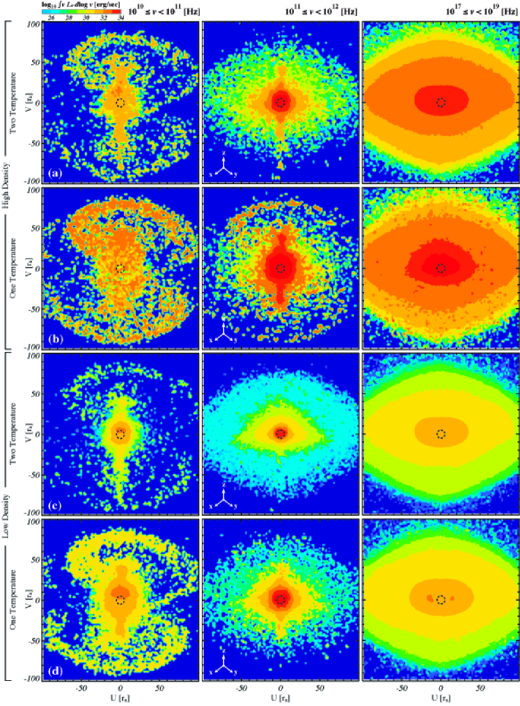
Figure 3: Synthetic images of four models [(a), (b), (c), and (d) from top to bottom] in different frequencies (left: $10^{10}\leq\nu<10^{11}$ [Hz]; centre: $10^{11}\leq\nu<10^{12}$ [Hz]; right: $10^{17}\leq\nu<10^{19}$ [Hz]) at the viewing angle of ($\theta$, $\phi$)$=$($\pi/3$, $\pi/4$). Colours indicate the power of escaping photon packets. A dotted circle with the radius $5r_{\rm s}$ indicates the canonical size of event horizon shadow.

Distinctive feature of non-axisymmetry is seen in all models at millimeter band. The non-axisymmetric structure in the magnetized accretion flows is also visible in Fig. 1. The apparent size of emission region in models (a) and (d) looks similar, whereas that in models (b) and (c) looks quite different. This is because the difference of density and temperature between model (a) and (d) compensate each other. On the other hand, non-axisymmetric feature cannot be seen in sub-millimeter band ($10^{11}-10^{12}$ Hz) except for model (b), but it has nearly spherical emission region around the gravitational centre. Again, the apparent size of emission region in model (a) and (d) looks quite similar. At both millimeter and sub-millimeter bands, the core of emission region correspond to the region of the strong magnetic field (see Fig. 1c), and the peak of emission region is slightly shifted from the gravitational centre.

All models represent the disc-like structure in X-ray band $10^{17}-10^{19}$ Hz. The apparent size of emission region in high-density models [(a) and (b)], and in low-density models [(c) and (d)] looks similar each other. This is because X-ray emission is produced by the Bremsstrahlung emission, which is sensitive to density, not to electron temperature. Interestingly, asymmetric structure can be seen only when electron temperature is equal to proton temperature [models (b) and (d)]. This feature is most likely to be produced by Compton scattering of low-energy photons generated by synchrotron emission (known as synchrotron self-Compton process: SSC).

3.2 Spectral energy distribution (SED)

In addition to the spatial distributions of radiative fields, we calculate the SED of our MHD model. In Fig. 4, the resultant SED is shown from radio to gamma-ray bands and also the observed spectra of Sgr A* are superimposed. The overall spectrum consist of several radiative processes, that is, self-absorbed synchrotron for $\nu\lower 2.0pt\hbox{$\,\buildrel\scriptstyle<\over{\scriptstyle\sim}\,$}10^{12}$ Hz, synchrotron for $10^{12}\lower 2.0pt\hbox{$\,\buildrel\scriptstyle<\over{\scriptstyle\sim}\,$}\nu\lower 2.0pt\hbox{$\,\buildrel\scriptstyle<\over{\scriptstyle\sim}\,$}10^{14}$ Hz, synchrotron self-Compton for $10^{14}\lower 2.0pt\hbox{$\,\buildrel\scriptstyle<\over{\scriptstyle\sim}\,$}\nu\lower 2.0pt\hbox{$\,\buildrel\scriptstyle<\over{\scriptstyle\sim}\,$}10^{17}$ Hz, and thermal Bremsstrahlung for $\nu\lower 2.0pt\hbox{$\,\buildrel\scriptstyle>\over{\scriptstyle\sim}\,$}10^{17}$ Hz. As we can see, time variability is different at each band. In optically thick region below the critical frequency $\nu_{\rm c}\approx 10^{12}$ Hz, there is a small time variation. When the frequency becomes higher, close to the critical frequency, the time variation becomes larger. Note that the variability at the lowest frequency edge $\sim 10^{9}$ Hz depends on the number of photon packets used in the calculation. Because of the strong self-absorption of synchrotron process, we cannot exclude the statistical errors in those frequency bands. Estimating from higher frequency regions, the variability is about two factors in magnitude. In optically thin region, on the other hand, time variation becomes prominent in the low-frequency band $10^{12}-10^{17}$ Hz and it becomes negligible in high-energy band $\lower 2.0pt\hbox{$\,\buildrel\scriptstyle>\over{\scriptstyle\sim}\,$}10^{17}$ Hz.

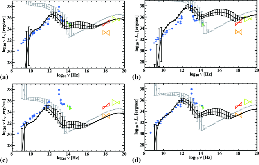
Figure 4: Spectral energy distributions for a different plasma model. (a) $\rho_{0}=8\times 10^{-15}{\rm[g\,cm^{-3}]}$ and $f_{\rm ep}=0.25$, (b) $\rho_{0}=8\times 10^{-15}{\rm[g\,cm^{-3}]}$ and $f_{\rm ep}=1$, (c) $\rho_{0}=8\times 10^{-16}{\rm[g\,cm^{-3}]}$ and $f_{\rm ep}=0.25$, and (d) $\rho_{0}=8\times 10^{-16}{\rm[g\,cm^{-3}]}$ and $f_{\rm ep}=1$. A black solid line and a grey dashed line indicate the emergent spectra and total emissivity spectra, respectively. Black bars associated with solid and dashed lines indicate the time variation at a given frequency band. Blue crosses and arrows indicate data taken by radio and infrared (IR) observations (Narayan et al. 1998 and reference therein). Green bars indicate data by near infrared observation (Eckart et al. 2006). X-ray observations of the flaring and the quiescent state by Chandra are depicted as red and orange “bow ties”, respectively (Baganoff et al. 2001) whereas gamma-ray observation of the flaring state by INTEGRAL is shown in light-green “bow ties” (Belandger et al. 2005).

The resultant SED of model (a) can nicely fit the observed SED in flaring state for all frequency range (Fig. 4a). The difference between the emergent spectra and the total emissivity spectra below the critical frequency is induced by the synchrotron self-absorption, whereas that in X-ray band is caused by the effect of viewing angle. Unlike the previous study of ADAF and OKM05, low-frequency bump in the millimeter band $10^{10}-10^{11}$ Hz is reconstructed successfully without considering non-thermal electrons. This is a main product of introducing a parameter $f_{\rm ep}$, which can account for spatially structured electron temperature distribution.

In order to explain two orders of magnitude difference in X-ray emission between flaring and quiescent states, the density need to be reduced by at least one order of magnitude, such as model (b) (see Fig. 4b). The resultant SED of model (b) can fit the X-ray spectra in quiescent state. However it under-predicts the radio to IR spectra for two-temperature plasma with $f_{\rm ep}=0.25$. Remaining option is to increase electron temperature so as to compensate the reduction of density, such as model (d) of one-temperature plasma with $f_{\rm ep}=1$ (see Fig. 4d). It turned out that the resultant SED of model (d) can successfully reconstruct the X-ray spectra of quiescent state as well as the radio and IR spectra. Although the underlying physics of electron heating is not clear, this is an outstanding result for the theory of hot accretion flows.

It is interesting to note that the X-ray variability does not strongly depend on the model parameter. Actually, all models except model (b) represent that the X-ray variability is very weak. In model (b), soft X-ray photons $\approx 10^{17}$ Hz are strongly contaminated by SSC photons because both density and electron temperature are increased so that scattering coefficient becomes large. Moreover, it seems that most of variabilities in ultraviolet band are produced by the scattered photons and also they are correlated with IR variabilities generated by synchrotron emission in all models. Note that the amplitude of variabilities (different between the maximum and the minimum power of escaping photons) in IR and UV bands does not change much in the range of our model parameter. Therefore, we suspect that the variability in the recent NIR observation (Eckart et al. 2005) are strongly affected by either the structure or the dynamics of the accretion flows.

4 Summary and Discussion

We have investigated three-dimensional radiative features of radiatively inefficient accretion flows modeled by MHD simulations. The synthetic images of all models show that the core of emission region in Sgr A* is larger than the size of the event horizon shadow, and is smaller than the radius of $100\,r_{\rm s}$. We have found that a non-axisymmetric structure of $m=1$ is associated with an elongated core emission in millimeter band. Remarkably, the peak location of the core emission in millimeter band $\approx 10^{11}$ Hz is slightly shifted from the gravitational centre. This is consistent with the baseline-correlated flux density diagram of the recent VLBI observation at 230 GHz (Doeleman et al. 2008).

We have also demonstrated for the first time that our 3-D MHD model with different density (namely different mass accretion rate) can reconstruct the observed broadband spectra including both the X-ray quiescent and flaring states, simultaneously. We have found that the X-ray flaring state corresponds to relatively high-mass accretion rate with a weak coupling between electron and proton temperature $f_{\rm ep}=0.25$, whereas the X-ray quiescent state corresponds to relatively low-mass accretion rate with a strong coupling between electron and proton temperature $f_{\rm ep}=1$. This is an opposite sense if one considers only the Coulomb coupling for electron heating. We will discuss this issue in the following.

Heating mechanism of electron in hot accretion flows has been investigated by many groups (Bisnovatyi-Kogan & Lovelace 1997; Quataert 1998; Gruzinov 1998; Blackman 1999; Quataert & Gruzinov 1999; Medvedev 2000). In ADAF/RIAF models, the turbulent viscosity primarily heats protons and then hot protons heats electrons via the Coulomb coupling between them. When the proton temperature becomes the virial temperature $\approx 10^{12}$ K, the electron-proton Coulomb relaxation time becomes much larger than the dynamical time (Spitzer 1956; Stepney 1983). As a result, the electron temperature decouple from the proton temperature. This is a well-known understanding of physics in hot accretion flows (Rees et al. 1982; Narayan et al. 1995). However, the spectra of hot accretion flows modeled by MHD simulations indicate that a coupling ratio $f_{\rm ep}$ is close to unity in both the flaring and quiescent state. Moreover, $f_{\rm ep}$ increases when the mass accretion rate decreases. This is an opposite sense in terms of plasma physics, because the electron-proton Coulomb relaxation time increases when the density decrease as $t_{\rm relax}\propto T_{\rm e}^{3/2}/\rho_{0}$. Therefore, our results imply that the alternative heating mechanism of electrons is requisite in order to keep the electron temperature being close to the proton temperature.

Recently, SQHS07 have found that significant fraction of dissipative energy generated by turbulent viscosity can be directly received by electrons. This can naturally explain the discrepancy of $f_{\rm ep}$ between our results and ADAF/RIAF models, because a fraction of energy received by electron is assumed to be typically $\delta\sim m_{\rm e}/m_{\rm p}\sim 10^{-3}$ in ADAF models (e.g., Narayan et al .1998). Although the detailed physics on the basis of viscous heating of electrons is in dispute, their results are worth to implement as subgrid physics of electron heating for 3-D global MHD simulations in the near future.

References

- Abramowicz (1995) Abramowicz, M. A., Chen, X., Kato, S., Lasota, J.-P., & Regev, O. 1995, ApJ, 438, L37
- Baganoff (2001) Baganoff, F. K., et al. 2001, Nature, 413, 45
- Baganoff et al. (2003) Baganoff, F. K., et al. 2003, ApJ, 591, 891
- Balbus (1991) Balbus, S. A., & Hawley, J. F. 1991, ApJ, 376, 214
- Balbus (1998) Balbus, S. A., & Hawley, J. F. 1998, Reviews of Modern Physics, 70, 1
- Balick (1974) Balick, B., & Brown, R. L. 1974, ApJ, 194, 265
- Bisnovatyi-Kogan & Lovelace (1997) Bisnovatyi-Kogan, G. S., & Lovelace, R. V. E. 1997, ApJ, 486, L43
- Blackman (1999) Blackman, E. G. 1999, MNRAS, 302, 723
- Bower et al. (2003) Bower, G. C., Wright, M. C. H., Falcke, H., & Backer, D. C. 2003, ApJ, 588, 331
- Bower (2004) Bower, G. C., Falcke, H., Herrnstein, R. M., Zhao, J.-H., Goss, W. M., & Backer, D. C. 2004, Science, 304, 704
- Bower et al. (2005) Bower, G. C., Falcke, H., Wright, M. C., & Backer, D. C. 2005, ApJ, 618, L29
- Doeleman (2008) Doeleman, S. S., et al. 2008, Nature, 455, 78
- Ghez (2003) Ghez, A. M., et al. 2003, ApJ, 586, L127
- Ghez (2004) Ghez, A. M., et al. 2004, ApJ, 601, L159
- Ghez (2008) Ghez, A. M., et al. 2008, ApJ, 689, 1044
- Gillessen (2009) Gillessen, S., Eisenhauer, F., Trippe, S., Alexander, T., Genzel, R., Martins, F., & Ott, T. 2009, ApJ, 692, 1075
- Gruzinov (1998) Gruzinov, A. V. 1998, ApJ, 501, 787
- Hawley (2000) Hawley, J. F. 2000, ApJ, 528, 462
- Hawley (2001) Hawley, J. F., & Krolik, J. H. 2001, ApJ, 548, 348
- Ichimaru (1977) Ichimaru, S. 1977, ApJ, 214, 840
- Igumenshchev (2003) Igumenshchev, I. V., Narayan, R., & Abramowicz, M. A. 2003, ApJ, 592, 1042
- Kato (2004) Kato, Y., Mineshige, S., & Shibata, K. 2004, ApJ, 605, 307
- Kato (2004) Kato, Y. 2004, PASJ, 56, 931
- Kato (2008) Kato, S., Fukue, J., & Mineshige, S. 2008, Black-Hole Accretion Disks — Towards a New Paradigm —, 549 pages, including 12 Chapters, 9 Appendices, ISBN 978-4-87698-740-5, Kyoto University Press (Kyoto, Japan), 2008.,
- Loeb & Waxman (2007) Loeb, A., & Waxman, E. 2007, Journal of Cosmology and Astro-Particle Physics, 3, 11
- Matsumoto (1999) Matsumoto, R. 1999, Numerical Astrophysics, 240, 195
- Matsumoto (1998) Matsumoto, M. & Nishimura, T. 1998, ACM Trans. on Modeling and Computer Simulation, 8, 3
- Machida (2000) Machida, M., Hayashi, M. R., & Matsumoto, R. 2000, ApJ, 532, L67
- Mahadevan (1998) Mahadevan, R. 1998, Nature, 394, 651
- Moscibrodzka (2007) Moscibrodzka, M., Proga, D., Czerny, B., & Siemiginowska, A. 2007, A&A, 474, 1 (MPCS07)
- Medvedev (2000) Medvedev, M. V. 2000, ApJ, 541, 811
- Narayan (1994) Narayan, R., & Yi, I. 1994, ApJ, 428, L13
- Narayan (1995) Narayan, R., Yi, I., & Mahadevan, R. 1995, Nature, 374, 623
- Ohsuga (2005) Ohsuga, K., Kato, Y., & Mineshige, S. 2005, ApJ, 627, 782 (OKM05)
- Pacholczyk (1970) Pacholczyk, A. G. 1970, Series of Books in Astronomy and Astrophysics, San Francisco: Freeman, 1970,
- Proga (2003) Proga, D., & Begelman, M. C. 2003, ApJ, 592, 767
- Pozdnyakov et al. (1977) Pozdnyakov, L. A., Sobol, I. M., & Syunyaev, R. A. 1977, Sov. Astron., 21, 708
- Quataert (1998) Quataert, E. 1998, ApJ, 500, 978
- Quataert & Gruzinov (1999) Quataert, E., & Gruzinov, A. 1999, ApJ, 520, 248
- Rees et al. (1982) Rees, M. J., Begelman, M. C., Blandford, R. D., & Phinney, E. S. 1982, Nature, 295, 17
- Rybicki & Lightman (1979) Rybicki, G. B., & Lightman, A. P. 1979, New York, Wiley-Interscience, 1979. 393 p.,
- Schödel et al. (2002) Schödel, R., et al. 2002, Nature, 419, 694
- Sharma et al. (2007) Sharma, P., Quataert, E., Hammett, G. W., & Stone, J. M. 2007, ApJ, 667, 714
- Shen (2005) Shen, Z.-Q., Lo, K. Y., Liang, M.-C., Ho, P. T. P., & Zhao, J.-H. 2005, Nature, 438, 62
- Spitzer (1956) Spitzer, L. 1956, Physics of Fully Ionized Gases, New York: Interscience Publishers, 1956,
- Stepney (1983) Stepney, S. 1983, MNRAS, 202, 467
- Stepney & Guilbert (1983) Stepney, S., & Guilbert, P. W. 1983, MNRAS, 204, 1269
- Stone (2001) Stone, J. M., & Pringle, J. E. 2001, MNRAS, 322, 461
- Yuan (2003) Yuan, F., Quataert, E., & Narayan, R. 2003, ApJ, 598, 301