Mean-field theory of a plastic network of integrate-and-fire neurons

Abstract

We consider a noise driven network of integrate-and-fire neurons. The network evolves as result of the activities of the neurons following spike-timing-dependent plasticity rules. We apply a self-consistent mean-field theory to the system to obtain the mean activity level for the system as a function of the mean synaptic weight, which predicts a first-order transition and hysteresis between a noise-dominated regime and a regime of persistent neural activity. Assuming Poisson firing statistics for the neurons, the plasticity dynamics of a synapse under the influence of the mean-field environment can be mapped to the dynamics of an asymmetric random walk in synaptic-weight space. Using a master-equation for small steps, we predict a narrow distribution of synaptic weights that scales with the square root of the plasticity rate for the stationary state of the system given plausible physiological parameter values describing neural transmission and plasticity. The dependence of the distribution on the synaptic weight of the mean-field environment allows us to determine the mean synaptic weight self-consistently. The effect of fluctuations in the total synaptic conductance and plasticity step sizes are also considered. Such fluctuations result in a smoothing of the first-order transition for low number of afferent synapses per neuron and a broadening of the synaptic weight distribution, respectively.

I Introduction

The brains of living animals are perhaps the most complex organs one can find. These are networks of neurons formed through the connecting synapses, and their proper functioning is crucial to survival. Theoretical studies of the dynamics of neural networks have contributed to our understanding of how these networks might function Vogels et al. (2005); Rabinovich et al. (2006). Recent progress in the study of synaptic plasticity is opening up new opportunities for understanding how these networks can form Abbott and Nelson (2000); Roberts and Bell (2002); Dan and Poo (2004). One of the most important aspects of a functional neural network is that the strength of its connections can change in response to the history of its activities, that is, it can learn from experience Amit and Brunel (1997); Malenka et al. (1999); Lynch (2004); Collingridge et al. (2004). Among the theories of neural learning, the best known, Hebbian theory, states that when a neuron partakes in the firing of another neuron, its ability of doing so increases Hebb (1949). An oversimplified version of the theory states that “cells that fire together, wire together” which is generally adequate for rate-based views of neurons Gerstner and Kistler (2002). However, the actual activities of neurons are described by “spikes”, that is, action potentials that are produced when the state of a neuron meets certain criteria, for example, when its membrane potential reaches a threshold value Izhikevich (2006). It was discovered that the exact timing of these spikes plays a great role in determining the synaptic plasticity, adding an element of causation to the correlation requirement of the learning process. That is, the presynaptic neuron must fire before the postsynaptic neuron for the former to actually take part in firing the later. In fact, it was discovered that a sharp change from potentiation to depression of the synaptic efficacy can occur as the firing time of the postsynaptic neuron precedes that of the presynaptic one Bi and Poo (2001); Roberts and Bell (2002); Dan and Poo (2004); Caporale and Dan (2008).

An important feature of Hebbian learning is the presence of positive feedback. That is, the stronger a synapse is, the more likely that it will be potentiated. Often in simulated plastic networks, this presents a possibility of runaway synaptic weights, which are often curbed through the introduction of cutoffs or other devices. In some schemes, the potentiation of a synapse is suspended when its weight exceeds a preset cutoff value Amarasingham and Levy (1998); Song et al. (2000); Rubin et al. (2001); Toyoizumi et al. (2007). While such cutoffs might be justified by physiological limitations of the cells, in simulation studies they often result in a pile-up of synaptic weights distributed near the cutoffs that is not observed in real biological neural networks Blum and Abbott (1996); Gerstner et al. (1996); Amarasingham and Levy (1998); Kempter et al. (1999); Song et al. (2000); van Rossum et al. (2000). Runaways or pile-ups can often be mitigated by softening the cutoff Kistler and van Hemmen (2000); Gerstner and Kistler (2002); Toyoizumi et al. (2007). Alternatively, it has been proposed from experimental observations that the potentiation and depression processes could be asymmetric, such that potentiation is an additive process to the current synaptic weight while depression is a multiplicative process. Such a mechanism was shown to produce a uni-modal distribution of synaptic weights free of pile-ups among the many afferent synapses of a single neuron when the inputs are driven by Poisson spiking sources van Rossum et al. (2000).

Besides viewing brains microscopically as networks of neurons as discussed above, efforts aimed at understanding the structure and function of a living brain also include studies at the macroscopic scale, for example of the interactions between different anatomical regions or even of the role played by the entirety of the brain as a vital organ Angevine and Cotman (1981); Hebb (1949). The contrast of the two scales is very analogous to the study of condensed matter systems, which has faced similar challenges of bridging our understanding of the microscopic with our observation of the macroscopic. Among various tools employed by theorists studying condensed matter systems, mean-field theory has been proven valuable in that it often allows one to obtain a quick grasp of what macroscopic states of the systems can be expected from the set of microscopic mechanisms they followHuang (1988). While it is well understood that mean-field theories could fail to predict correct scaling behavior of systems in critical states, where fluctuations and long-range correlations are important, they generally are adequate (and often the first step in a systematic procedure) in qualitatively describing the system in stable phases, where fluctuations are of limited range, and useful in revealing the structure of the phase spaces of the systems. The later is especially desirable for biological systems where large numbers of empirical parameters and, consequently, vast phase spaces are often involved in microscopic models of the systems.

In the current study, we consider a network of integrate-and-fire neuronsBurkitt (2006) driven by Poisson noise of fixed frequency for all neurons. The interaction between the neurons is taken to follow the neural transmission model proposed by Tsodyks, Uziel, and Markram Tsodyks et al. (2000) (the TUM model), which can account for the saturation effect of neural transmitter and the short-term depression of synaptic conductance. While our approach can handle alternative choices, the synaptic weights between the neurons are allowed to evolve following the spike-timing-dependent plasticity rules proposed by Bi and coworkers Bi and Poo (1998); van Rossum et al. (2000). A mean-field theory is used to determine the self-consistent average firing rate of the neurons. The noise driven firings dominate the small synaptic weight regime, while self-sustaining firing activity is triggered in the large synaptic weight regime. As the mean synaptic weight of the network is varied, the mean-field theory predicts a hysteresis for the transition between regimes of noise dominance and self-sustaining activity. Within the mean-field environment, assuming the neurons are firing with Poisson statistics, the dynamics of a single synapse can be viewed as a random walk process in synaptic-weight space. Under the small-jump assumption, we use the master equation to calculate the drift and diffusion coefficient for the random walk. The resulting Fokker–Planck equation allows us to predict the stationary synaptic-weight distribution of the process and close the self-consistency with the requirement that the stationary distribution reproduces the mean synaptic weight characterizing the mean-field environment. For the plasticity rules and ranges of the parameters we considered, the synaptic weights form a narrow distribution, having a width proportional to square root of the plasticity rate. Finally, we extend the mean-field approximation to include the effect of fluctuations in the synaptic conductance as well as the variations of jump sizes in the random walk of synaptic weights.

Of course, despite our mention of brains of living creatures in our introduction, the current analysis cannot hope to address issues of dynamics involved in such a venue for myriad reasons. Among others, here we imagine homogeneous, stationary networks, which is surely not the case in brain. However, there are continuing, revealing experiments on cultured neural networks with perhaps several hundred individual neurons in which all-to-all coupling is not an unreasonable approximation or starting point Bi and Poo (1998); Segev et al. (2001); Shefi et al. (2002); Beggs and Plenz (2003); Lai et al. (2006). This class of experiments represents an important step and will continue to provide important insights into the behavior of more complicated networks. Our aims are to improve the understanding of the stationary, statistical properties of such plastic network and ultimately address dynamical behavior during formation. Furthermore, cultured networks are on a scale approachable by the modeling, numerical and analytic work such as presented here. By analogy with a variety of familiar statistical mechanical models, sufficiently large homogeneous networks in which the number of “neighbors” of a particular element grows proportionally to the number of elements in the thermodynamic limit, are expected to be well-described by the type of mean-field analysis employed in this study (see, e.g., chapter 3 of Baker (1990)). In a separate publication we will present results of extensive numerical simulations on integrate-and-fire (and other representative neuron model) networks, the results of which can be put in the proper perspective via comparison with the calculations presented here and with results of in vitro experiments.

The remainder of this paper is laid out as follows. In Section II, we describe the model of the plastic network, which consists of (i) the dynamics of the membrane potential, (ii) the model of synaptic transmission, and (iii) the plasticity rules. In Section III, we apply the mean-field method to a network with fixed synaptic weights and determine the state of the system through response functions deduced from the dynamics of neuron and synaptic transmission under a given mean synaptic weight. In Section IV, we map synaptic plasticity to a random walk process in synaptic-weight space, determine the stationary synaptic-weight distribution, and close the self-consistency in the mean synaptic weight of the network. In Section V, we expand the mean-field theory to include the consideration of fluctuations in total synaptic current of a neuron and fluctuations in step sizes of synaptic weight changes. Finally, we summarize and conclude in Section VI.

II Model

We consider a noise-driven plastic network of integrate-and-fire neurons. The neurons are coupled using the TUM model of neural transmission Tsodyks et al. (2000); Volman et al. (2007), described below. The noise is modeled by randomly forced firing of the neurons following Poisson statistics at a fixed frequency.

II.1 Integrate-and-fire neuron

The integrate-and-fire model is a single-compartment neuron model where the state of a neuron $i$ is described by a membrane potential $V_{i}$. The dynamics of the membrane potential follows the differential equation of a leaky integrator Dayan and Abbott (2001)

$$\tau_{m}\frac{dV_{i}}{dt}=V_{0}-V_{i}+R_{m}I_{\mathrm{syn}},$$ (1)

where $\tau_{m}$ is the leak time for the membrane charge, which is given by the product of the total membrane capacitance $C_{m}$ and resistance $R_{m}$, while $V_{0}$ is the resting potential when the neuron is in the quiescent state. The total synaptic current $I_{\mathrm{syn}}$ is a sum over each afferent synapse $j$ for the neuron $i$

$$I_{\mathrm{syn}}=\frac{1}{R_{m}}\sum_{j}w_{j,i}Y_{j,i}\left(\mathcal{R}_{j,i}-V_{i}\right),$$ (2)

where, for the synapse connecting neuron $j$ to $i$, $w_{j,i}$ is the synaptic weight, $\mathcal{R}_{j,i}$ is the reversal potential for the ion channels, and $Y_{j,i}$ is the fraction of active transmitters. The dimensionless synaptic weight $w_{j,i}$ can be interpreted as the maximum synaptic conductance, achieved when $Y_{j,i}=1$, measured in units of the membrane conductance $R_{m}^{-1}$ of the neuron. In the current study, we consider cases in which there is only one type of ion channel at all synapses so that they share the same reversal potential $\mathcal{R}_{j,i}=\mathcal{R}$. In these cases, the difference of membrane potential from the reversal potential can be factored out and Eq. (1) becomes

$$\tau_{m}\frac{dV_{i}}{dt}=V_{0}-V_{i}+G_{i}\left(\mathcal{R}-V_{i}\right),$$ (3)

where

$$G_{i}\equiv\sum_{j}w_{j,i}Y_{j,i}$$ (4)

is the total synaptic conductance (in units of $R_{m}^{-1}$).

In this model, a neuron fires when its membrane potential reaches a threshold value, $V_{\mathrm{th}}$. Then, its membrane potential drops immediately to a reset value, $V_{\mathrm{r}}$. The action potential of the integrate-and-fire model is assumed to be instantaneous and is not modeled explicitly. The spike train produced by the neuron $i$ is defined as the function

$$S_{i}\equiv\sum_{n}\delta\left(t-t_{i,n}\right)$$ (5)

where $t_{i,n}$ is the time when the neuron $i$ fires for the $n$-th time.

II.2 Tsodyks–Uziel–Markram model of neural transmission

The fractions $Y_{j,i}$ of the active transmitters are described by the TUM model Tsodyks et al. (2000) of neural transmission, where the transmitters are distributed in three states: “active”, with the fraction $Y$; “inactive”, with the fraction $Z$; and “ready-to-release”, with the fraction $X$. For a synapse with presynaptic neuron $j$ and postsynaptic neuron $i$, these fractions follow the dynamics Tsodyks et al. (2000)

$$\frac{dX_{j,i}}{dt} = \frac{Z_{j,i}}{\tau_{R}}-uS_{j}X_{j,i}$$

$$\frac{dY_{j,i}}{dt} = -\frac{Y_{j,i}}{\tau_{D}}+uS_{j}X_{j,i}$$ (6)

$$\frac{dZ_{j,i}}{dt} = \frac{Y_{j,i}}{\tau_{D}}-\frac{Z_{j,i}}{\tau_{R}},$$

where $\tau_{D}$ is the decay time of active transmitters to the inactive state, $\tau_{R}$ is the recovery time for the inactive transmitters to the ready-to-release state, and $u$ is the fraction of ready-to-release transmitters that is released to the active state by each presynaptic spike. With the conservation rule

$$X_{j,i}+Y_{j,i}+Z_{j,i}=1,$$ (7)

there are two independent variables per synapse. Since the multiplying factor of the spike train $S_{j}$ in the dynamics of $X_{j,i}$ depends on $X_{j,i}$ itself, which is discontinuous when there is a $\delta$-function in $S_{j}$ due to a spike at given time $t$, we must specify how the value of $X_{j,i}$ should be evaluated at the time of the spike. Consistent with the TUM dynamics, the values of the factors multiplying $S_{j}$ at the discontinuities are to be evaluated immediately before the discontinuities.

The TUM model is very flexible. Since the variable $Y$ represents a fraction in the TUM model, its value can saturate. As a result, an increase in the firing of the presynaptic neuron can only produce a less-than-linear increase of the active transmitters. However, a linearity of active transmitters on the firing rate can be recovered in the $u\rightarrow 0$ limit, maintaining the average level of the synaptic conductance by keeping the product $w_{j,i}u$ constant. Additionally, the presence of the inactive state, $Z$, mimics the short-term depression of neural transmission, where repeated firings of the presynaptic neuron over a short period of time will reduce the maximum value attainable by $Y$ temporarily through depositing the transmitters into the inactive state before their recovery. Finally, manipulating $\tau_{R}/\tau_{D}$ can reproduce a model with a single, saturating “species” Y (see below).

Since the dynamics (6) depend only on the spike train of the presynaptic neuron $j$, without external disturbance all the efferent synapses of a neuron should have the same values of transmitter fractions. Thus, we can drop the subscript $i$ from dynamics (6) and regard these fractions as the properties of the presynaptic neuron $j$. Such simplification is not applicable for transmitter dynamics that depend, for example, on the postsynaptic neuron, that have synaptic-weight-dependent parameters, or synapse-dependent noise. These complications are not considered here.

II.3 Noise

While the integrate-and-fire and TUM dynamics are both deterministic, we model the stochasticity of the network with additional noise driven firing events following Poisson statistics with the frequency $\lambda_{N}$ for each neuron. The noise driven firings are treated the same way as threshold firings, that is, the membrane potentials are brought instantaneously to the reset value $V_{\mathrm{r}}$ and the firing times are included in the spike trains (5) of the transmitter dynamics (6).

II.4 Spike-timing-dependent plasticity

It has been observed experimentally that the change of synaptic efficacy depends on the precise timing between the presynaptic and postsynaptic spikes Bi and Poo (2001). When a presynaptic spike precedes a post-synaptic spike, following van Rossum, Bi, and Turrigiano van Rossum et al. (2000), we take the synapse to be potentiated by an amount proportional to $e^{-\Delta t/\tau_{A}}$ where $\Delta t$ is the timing difference between the two spikes and $\tau_{A}$ is the size of the potentiation time window. Similarly when a postsynaptic spike precedes a presynaptic spike, the synapse is taken to be depressed by an amount proportional to $e^{-\Delta t/\tau_{B}}$ where $\tau_{B}$ is the size of the depression time window Bi and Poo (1998); van Rossum et al. (2000). One reasonable mechanism for the cell to determine the interval between spikes is to imagine the cell evaluates the concentration of a decaying chemical species released at the first spike Pfister and Gerstner (2006). Following such a mechanism, the synaptic changes proposed in van Rossum et al. (2000) can be produced for the synaptic weight $w_{j,i}$ by the dynamical equation

$$\frac{dw_{j,i}}{dt}=\Delta A_{j}S_{i}-rw_{j,i}B_{i}S_{j},$$ (8)

where $\Delta$ is the potentiation constant for causal spike pairs, $r$ is the depression factor for anti-causal spike pairs, while $A$s and $B$s are the amplitudes of such (assumed) chemical species controlling the magnitude of potentiation and depression. These amplitudes are assumed to follow the dynamics Pfister and Gerstner (2006)

$$\frac{d\sigma_{j}}{dt}=-\frac{\sigma_{j}}{\tau_{\sigma}}+f_{\sigma}S_{j},\;\sigma=A,B$$ (9)

where different choices of the spike increments $f_{\sigma}$ lead to different schemes of spike pairing. For example, $f_{\sigma}=1$ leads to “all-to-all” pairing of presynaptic and postsynaptic spikes while $f_{\sigma}=1-\sigma$ leads to “nearest-neighbor” pairing of spikes Pfister and Gerstner (2006). We note the stochastic differential equations in Eqs. (8) and (9) above should follow Itô’s interpretation van Kampen (2007). That is, when the value of $\sigma$ jumps because of a spike in $S$, the value of $f_{\sigma}$, which determines the size of the jump, is evaluated immediately before the jump. The effects of the two choices of $f_{\sigma}$ are identical when spike pairs are far and apart but differ when possible spike pairs are close compared with the decay time $\tau_{\sigma}$ of the respective timing chemicals. With the choice $f_{\sigma}=1$, the values of $A$ or $B$ can increase linearly with the frequency of spikes without limit. On the other hand, for the choice $f_{\sigma}=1-\sigma$, the value of $\sigma$ will never exceed 1, its value immediately after a single spike. It is reasonable to expect, in a realistic setting, that the values of $A$ or $B$ will increase with increasing spike rates, but they should saturate and be limited to some physiologically determined maximum values with further increase in spike rates. Assuming spike increments $f_{\sigma}=u_{\sigma}\left(1-\sigma\right)$ with $u_{\sigma}<1$ can produce this behavior. The parameter $u_{\sigma}$ can be interpreted as the mean fraction of chemicals released at each presynaptic firing relative to the amount that can possibly be produced without $\sigma$ exceeding its maximum value of $1$.

Additionally, certain effects of fatigue can also be expected in synaptic plasticity. Froemke et al. (2006) That is, while $\sigma$ ($=$$A$ or $B$) can saturate when the spike rate increases, the saturation value itself can be expected to decrease when a high spiking rate is sustained for an extended period of time Tsodyks et al. (2000); Volman et al. (2007). Such effect can be modeled by assuming an additional inactive state $I_{\sigma}$, which takes up a fraction of $\sigma$ that can be produced for each spike, so that the increment becomes $f_{\sigma}=u_{\sigma}\left(1-\sigma-I_{\sigma}\right)$. One can assume simple dynamics for $I_{\sigma}$, given by

$$\frac{dI_{\sigma}}{dt}=\frac{\sigma}{\tau_{I\sigma}}-\frac{I_{\sigma}}{\tau_{R\sigma}}$$ (10)

so that $I_{\sigma}$ is fed by the presence of $\sigma$ with the rate $\tau_{I\sigma}^{-1}$ and decays with a recovery time constant $\tau_{R\sigma}$. One expects that the rate of $\sigma$’s feeding into the inactive state [first term on the right of Eq. (10)] should be less than the rate of its own decay [first term on the right of Eq. (9)], so we require the condition $\tau_{I\sigma}\geq\tau_{\sigma}$.

The considerations outlined above conspire to produce a variant of the TUM model similar to what we have used for the neural transmitters apart from possibly different values of the constants involved. In the current simulation study of plastic integrate-and-fire networks, we retain the qualitative structure of the system but simplify by assuming $\tau_{\sigma}=\tau_{I\sigma}=\tau_{D}$, $\tau_{R\sigma}=\tau_{R}$, and $u_{\sigma}=u$ so that the same values of $Y_{i}$ calculated for the neural transmitter in the TUM model can be used as surrogates for $A_{i}$ and $B_{i}$ in the synaptic plasticity yielding

$$\frac{dw_{j,i}}{dt}=\Delta Y_{j}S_{i}-rw_{j,i}Y_{i}S_{j}.$$ (11)

These simplifications reduce the amount of computation required without sacrificing qualitative and semi-quantitative analysis.

To summarize, our system of equations reduces to Eqs. (3)–(7) and (11). The “control parameter” in subsequent analysis will turn out to be

$$w^{\star}\equiv\frac{\Delta}{r},$$ (12)

which, when fixed, leaves the depression factor $r$ as an overall control of rate of plasticity.

III Mean-field approximation

III.1 Single neuron response function

To formulate a mean-field approximation, we assume that the firing rates of the neurons are given by the same mean-field value $\bar{\lambda}$ and that all the synapses have the same synaptic weight $\bar{w}$. The total synaptic conductance $G$ of a singled-out postsynaptic neuron is a function of time and jumps whenever there is a firing of a presynaptic neuron and subsequently decays with the time constant $\tau_{m}$ as in Eq. (3). Consider the limit of large number $K$ of afferent synapses per neuron while keeping the product $\bar{w}K$ constant. Then, the total frequency of all presynaptic firings is $K\bar{\lambda}\rightarrow\infty$. In this limit, the jump sizes of $G$, being proportional to $\bar{w}$, approach $0$ while the rate of making the jumps diverges. For fixed $\bar{\lambda}$ and $\bar{w}K$, we may thus ignore fluctuations and consider $G$ as a constant over time.

For a constant total synaptic conductance $G$, the firing frequency of an integrate-and-fire neuron can be solved exactly by setting the initial membrane potential to $V\left(0\right)=V_{\mathrm{r}}$, the reset value, and finding the time $\tau$ it takes to reach the firing threshold $V\left(\tau\right)=V_{\mathrm{th}}$. The solution of Eq. (3) is given by

$$\tau=-\frac{\tau_{m}}{G+1}\ln\left(\frac{\tilde{V}\left(G\right)-V_{\mathrm{th}}}{\tilde{V}\left(G\right)-V_{\mathrm{r}}}\right)$$ (13)

when $\tilde{V}\left(G\right)\geq V_{\mathrm{th}}$, where

$$\tilde{V}\left(G\right)\equiv\frac{V_{0}+G\mathcal{R}}{G+1}$$ (14)

is the resting value for the membrane potential under the constant conductance $G$. For $\tilde{V}<V_{\mathrm{th}}$, we have $\tau=\infty$ since the neuron never fires. In addition to firings due to crossing the threshold, the period $\tau$ can be cut short by Poisson noise of frequency $\lambda_{N}$ as the membrane potential sweeps from $V_{\mathrm{r}}$ to $V_{\mathrm{th}}$. Given Poisson statistics, the average interval $\bar{\tau}$ between all firings (either threshold-crossing or noise-driven) is given by

$$\bar{\tau} = \int_{0}^{\tau}dt\lambda_{N}te^{-\lambda_{N}t}+\tau\int_{\tau}^{\infty}dt\lambda_{N}e^{-\lambda_{N}t}$$ (15)

$$= \lambda_{N}^{-1}\left(1-e^{-\lambda_{N}\tau}\right),$$

and the firing frequency $\lambda$ of the neurons is given by

$$\lambda\left(G\right)=\lambda_{N}\left[1-\left(\frac{\tilde{V}\left(G\right)-V_{\mathrm{th}}}{\tilde{V}\left(G\right)-V_{\mathrm{r}}}\right)^{\frac{\lambda_{N}\tau_{m}}{G+1}}\right]^{-1}$$ (16)

for $\tilde{V}\geq V_{\mathrm{th}}$, and by $\lambda=\lambda_{N}$ otherwise. (See Fig. 1.)

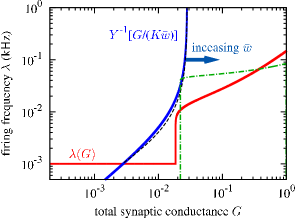
Figure 1: Firing frequency $\lambda\left(G\right)$ of an integrate-and-fire neuron under constant total synaptic conductance $G$ given by Eq. (16). Also shown are mean-field active synaptic transmitter fractions $Y\left(\lambda\right)$ (for $K=31$, $\bar{w}=0.01$) driven by a Poisson spike train of frequency $\lambda$ given by (17). The dashed line represents a numerically calculated correction to $Y\left(\lambda\right)$ due to the periodic firing of the neuron when driven by constant total synaptic conductance $G$. The parameters are listed in Table 1. The arrow indicates that the curve shifts to the right for increasing $\bar{w}$. The dot-dashed line is the neuron response function numerically calculated for the Morris–Lecar model used in Volman et al. (2007) with a slightly higher background current.

Table 1: Values of parameters used in calculations

integrate & fire				TUM model
resting potential $V_{0}$:	-55 mV			decay time $\tau_{D}$:	20 ms
leak time $\tau_{m}$:	20 ms			recovery time $\tau_{R}$:	200 ms
firing threshold $V_{\mathrm{th}}$:	-54 mV			release fraction $u$:	0.5
reset potential $V_{\mathrm{r}}$:	-80 mV			noise frequency $\lambda_{N}$:	1 Hz
reversal potential $\mathcal{R}$:	0 mV			plasticity rate $r$:	0.01

The function $\lambda\left(G\right)$ obtained in (16) characterizes the mean-field response of the integrate-and-fire network model in the current study , but similar functions can be obtained analytically or numerically for different neuron models, such as, the Hodgkin–Huxley, Morris–Lecar, or FitzHugh–Nagumo models (see, e.g., Gerstner and Kistler (2002); Izhikevich (2004)). (An example of a numerically calculated response function for a Morris–Lecar neuron is included in Fig. 1.)

III.2 Synapse response function

To obtain the mean-field active transmitter fraction $\bar{Y}$ of a neuron, we further approximate the firing of the neurons as having Poisson statistics described by the mean-field firing rate $\bar{\lambda}$ Rubin et al. (2001). Keeping $Y$ and $Z$ as the independent variables for the TUM model, the stochastic dynamics (6) can be averaged over an ensemble of Poisson spike trains with $\left\langle S\right\rangle=\lambda$ for the presynaptic neuron to yield the functions

$$Y\left(\lambda\right)=\frac{u\tau_{D}\lambda}{1+u\left(\tau_{D}+\tau_{R}\right)\lambda}$$ (17)

and $Z\left(\lambda\right)=\frac{\tau_{R}}{\tau_{D}}Y\left(\lambda\right)$ for the average active ($Y$) and inactive ($Z$) transmitter fractions. The function $Y\left(\lambda\right)$ characterizes the mean-field response of a synapse . The value of the active transmitter fraction for a mean-field network can be obtained through the relation

$$\bar{Y}=Y\left(\bar{\lambda}\right).$$ (18)

III.3 Self-consistency condition

The total synaptic conductance of a neuron in a mean-field network with $K$ afferent synapses per neuron is given by

$$\bar{G}=K\bar{w}\bar{Y}=K\bar{w}Y\left(\bar{\lambda}\right),$$ (19)

which can be substituted into Eq. (16) to complete the self-consistency condition closing the set of Eqs. (16), (17), and (19). The curve for Eq. (19) is also shown in Fig. 1, and the intersections with the neuron response function $\lambda\left(G\right)$ represent fixed points of the network activities, $\bar{\lambda}$, given the mean-field synaptic weight $\bar{w}$.

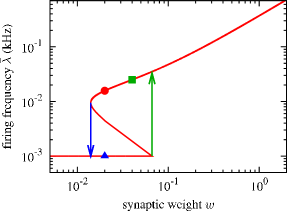
Figure 2: Mean-field firing frequency $\bar{\lambda}$ as a function of mean-field synaptic weight $\bar{w}$ determined by the intersections of neuron response function and synapse response function as plotted in Fig. 1 for $K=31$. The two arrows show the region of hysteresis where two stable fixed points, the noise-dominating lower fixed point and the persistently active upper fixed point, coexist. The symbols will be used in connection with Figs. 4 and 7.

The function $\bar{\lambda}\left(\bar{w}\right)$ is shown in Fig. 2. The mean-field theory predicts a first-order phase transition and hysteresis as the mean-field synaptic weight $\bar{w}$ is varied. At low synaptic weight, the activities of the network are dominated by the external noise. As the synaptic weight is increased, a pair of new fixed points emerge at higher firing frequencies. Among the three fixed points, only the upper and the (noise-dominated) lower fixed points are stable. As the synaptic weight is increased further, the lower fixed point eventually is annihilated by the unstable (middle) fixed point leaving only the upper fixed point representing higher firing activities.

IV Random walk in synaptic weight space

Given the mean-field firing frequency $\bar{\lambda}$ for a fixed mean synaptic weight $\bar{w}$, motivated by the Bethe–Peierls approximation Huang (1988), we consider a single synapse within such a mean-field environment as illustrated in Fig. 3.

Figure 3: We consider the dynamics of a single synapse of synaptic weight $w$ in a mean-field environment.

The time-dependence of the synaptic weight is governed by Eq. (8) and the simplification embodied in Eq. (11). With the assumption of Poisson spike trains produced by both the presynaptic and postsynaptic neurons, the dynamics of the synaptic weight maps onto an asymmetric random walk (jump process) in $w$-space with $w$-dependent jump rates and jump sizes van Kampen (2007). From Eqs. (8) and (11), the synaptic weight increases by $\Delta\,A_{2}=\Delta\,Y_{2}$ whenever the postsynaptic neuron fires and decreases by $rwB_{1}=rwY_{1}$ whenever the presynaptic neuron fires. As the presynaptic neuron is driven by the mean-field environment, its firing frequency $\lambda_{2}$ is given by the mean-field firing frequency $\bar{\lambda}$. On the other hand, the postsynaptic neuron is partly driven by the synapse in question (Fig. 3), thus its firing frequency $\lambda_{1}$ is $w$ dependent. As calculated from the neuron response function $\lambda\left(G\right)$, this firing rate is given by

$$\lambda_{1}=\lambda\left(\left[\left(K-1\right)\bar{w}+w\right]\bar{Y}\right),$$ (20)

where, even though the synaptic weight $w$ is singled out from among the $K$ afferent synapses, all of the presynaptic neurons are from the mean-field environment (see Fig. 3) with the active transmitter fraction $\bar{Y}$. As for the step sizes, since $A_{2}$ depends on the firing of the presynaptic neuron, its value is given by the mean-field value $\bar{Y}$. On the other hand, $B_{1}$ is determined by the firing of postsynaptic neuron; therefore its value is also $w$ dependent and given by $B_{1}=Y\left(\lambda_{1}\right)$. As mentioned earlier, we set $A=B=Y$ to reduce the number of variables and computational intensiveness. In general, the system can have different characteristic functions $A\left(\lambda\right)$ and $B\left(\lambda\right)$ for potentiation and depression.

IV.1 Mean-field synaptic weight

While the “random walk” of synaptic weight is under the influence of the mean-field environment, a self-consistency condition requires the average value of the singled-out synaptic weight from the random walk process to be the same as the assumed mean-field value $\bar{w}$. Assuming a normalized stationary synaptic-weight distribution from the random walk, $P_{s}\left(w\right)$, which is $\bar{w}$-dependent, the self-consistency requires

$$\bar{w}=\left\langle w\right\rangle\equiv\int_{0}^{\infty}wP_{s}\left(w;\bar{w}\right)dw.$$ (21)

The stationary synaptic weight distribution, following the stochastic dynamics (11), can not be easily determined even with the assumption of Poisson spike trains. However, straightforward numerical simulations of a system of a single synapse and two Poisson neurons can be used to obtain the stationary distribution $P_{s}\left(w;\bar{w}\right)$ to any reasonable precision.

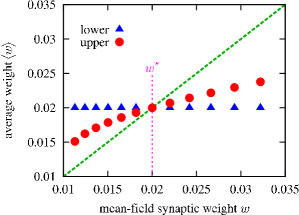
Figure 4: Average synaptic weight from the simulation of a single synapse between two Poisson neurons as shown schematically in Fig. 3 versus the mean-field synaptic weight $\bar{w}$ for $w^{\star}=0.02$. The mean-field firing frequencies $\bar{\lambda}$ used in the single synapse simulations are given by Fig. 2, and the results for both the upper and lower fixed points (marked by corresponding symbols in Fig. 2) are plotted.

Figure 4 shows typical plots of the average synaptic weight from the random walk process as a function of the mean-field synaptic weight $\bar{w}$. Notice that the symbols are lower (higher) than the dashed line on the left (right) meaning that a deviation of $\bar{w}$ from $w^{\star}$ results in a smaller deviation of $\left\langle w\right\rangle$ from $w^{\star}$. Hence, the $\bar{w}=w^{\star}$ is a stable solution for the condition (21).

IV.2 Fokker–Planck equation

Since the synaptic weight dynamics (8) [or (11)] only depend on the current weight of the synapse (a Markov process), we can approximate the dynamics of the weight distribution for small jumps with a master equation ignoring higher-order moments in the Kramers–Moyal expansion (see, e.g., van Kampen (2007)). A Fokker–Planck equation formalism has been applied to populations of neurons in previous studies of the distributions in membrane potential Fourcaud and Brunel (2002); Brunel and Hansel (2006); Cateau and Reyes (2006). Here we apply this type of formalism to a population of plastic synapses similar to the work by Rubin, Lee, and Sompolinsky Rubin et al. (2001).

Equation (8) or its simplification (11) can be viewed as a stochastic equation governing the jumps in synaptic weight space upon arrival of spikes and which allows us to calculate the drift

$$v \equiv \lim_{\Delta t\rightarrow 0}\frac{\left\langle w\left(\Delta t\right)-w\right\rangle_{w\left(0\right)=w}}{\Delta t}$$ (22)

$$= \Delta\bar{Y}\lambda_{1}-rwY\left(\lambda_{1}\right)\bar{\lambda},$$

where $\lambda_{1}$ is given by Eq. (20). One also has for the diffusion coefficient (arising from the second moment of the synaptic weight changes)

$$D \equiv \frac{1}{2}\lim_{\Delta t\rightarrow 0}\frac{\left\langle\left[w\left(\Delta t\right)-w\right]^{2}\right\rangle_{w\left(0\right)=w}}{\Delta t}$$ (23)

$$= \frac{1}{2}\Delta^{2}\bar{Y}^{2}\lambda_{1}+\frac{1}{2}r^{2}w^{2}\left[Y\left(\lambda_{1}\right)\right]^{2}\bar{\lambda}.$$

The dynamics of the synaptic weight distribution $P\left(w\right)$ is then approximated for small jumps by the Fokker–Planck equation

$$\frac{\partial P\left(w\right)}{\partial t}=-\frac{\partial}{\partial w}\left[vP\left(w\right)\right]+\frac{\partial^{2}}{\partial w^{2}}\left[DP\left(w\right)\right]$$ (24)

when higher-order moments in the Kramers–Moyal expansion are ignored. Consider the stationary state $P_{s}\left(w\right)$ of the weight distribution. The Fokker–Planck equation (24) can be integrated once to yield

$$vP_{s}\left(w\right)=\frac{\partial}{\partial w}\left[DP_{s}\left(w\right)\right]+\textrm{const.},$$ (25)

which is formally solved by

$$P_{s}\left(w\right)\propto\frac{1}{D}e^{\int^{w}dw^{\prime}v\left(w^{\prime}\right)/D\left(w^{\prime}\right)}.$$ (26)

The peak positions of the distribution (26), $\hat{w}$, (if they exist) are given by $v\left(\hat{w}\right)=D^{\prime}\left(\hat{w}\right)$. Since the diffusion coefficient (23) is one-order higher in the plasticity rate $r$ compared to the drift (22), under the small jump approximation, the peak positions are given approximately by the zeros of $v$. When $\bar{w}=w^{\star}\equiv\Delta/r$, we can verify that the drift (22) is zero and thus the distribution $P_{s}\left(w\right)$ should peak at $w=\bar{w}$. We can expand $v$ and $D$ in powers of $w-\bar{w}$ and keep only the first order terms. The exponent of Eq. (26) becomes

$$\int^{w}dw^{\prime}\frac{w^{\star}-w^{\prime}}{r\bar{Y}{w^{\star}}^{2}}=\frac{-\left(w^{\star}-w\right)^{2}}{2r\bar{Y}{w^{\star}}^{2}}+\mbox{const.},$$ (27)

which results in a Gaussian distribution for $P_{s}\left(w\right)$. The distribution is very narrow; the width of the distribution is given by

$$\Delta w\simeq\sqrt{r\bar{Y}}w^{\star}$$ (28)

which corresponds to only about 1% of $w^{\star}$ for the parameters we have considered in Table 1 above. Simulations for a fully connected network using the same model and parameters yield a width about five times larger but with the same scaling power in $r$ in the noise-dominated regime Chen and Jasnow . We will return to this point below.

IV.3 Stability analysis within mean-field theory

The condition $v\left(\hat{w}\right)=0$ for the peak position $\hat{w}$ of the synaptic-weight distribution gives rise to

$$\Delta\bar{Y}\hat{\lambda}_{1}=r\hat{w}Y\left(\hat{\lambda}_{1}\right)\bar{\lambda},$$ (29)

where $\hat{\lambda}_{1}=\lambda_{1}\left(\hat{w}\right)$. Using the mean-field response function (17) for the synapses, we get

$$\hat{w}=w^{\star}\frac{1+u\left(\tau_{D}+\tau_{R}\right)\hat{\lambda}_{1}}{1+u\left(\tau_{D}+\tau_{R}\right)\bar{\lambda}}.$$ (30)

It is straightforward to verify that when the mean-field synaptic strength is given by $\bar{w}=w^{\star}$, the peak position is given by $\hat{w}=\bar{w}$, providing a self-consistent solution. To determine the stability of the solution, we start with a small deviation $\delta\bar{w}$ of $\bar{w}$ from $w^{\star}$ and find the resultant deviation $\delta\hat{w}$ of the peak position $\hat{w}$ from $\bar{w}$. Assuming the neuron response function $\lambda\left(G\right)$ is smooth around the mean-field total conductance $\bar{G}=K\bar{w}\bar{Y}$, the firing frequency of the postsynaptic neuron can be expanded

$$\hat{\lambda}_{1}\approx\bar{\lambda}+\lambda^{\prime}\left(\bar{G}\right)\delta\hat{w}\bar{Y}$$ (31)

where $\lambda^{\prime}$ is the first derivative of the mean-field response function $\lambda\left(G\right)$. The mean-field response function $Y\left(\lambda\right)$ for the active transmitter can also be expanded as

$$Y\left(\lambda_{1}\right)=\bar{Y}\left[1+Y^{\prime}\left(\bar{\lambda}\right)\lambda^{\prime}\left(\bar{G}\right)\delta\hat{w}\right].$$ (32)

The condition $v\left(\hat{w}\right)=0$ results in

$$\bar{w}-w^{\star}=\delta\bar{w}=\left\{w^{\star}\lambda^{\prime}\left(\bar{G}\right)\left[\frac{\bar{Y}}{\bar{\lambda}}-Y^{\prime}\left(\bar{\lambda}\right)\right]-1\right\}\delta\hat{w}.$$ (33)

For the $\bar{w}=w^{\star}$ solution to be stable, $\delta\hat{w}$ and $\delta\bar{w}$ should be of opposite signs so that the perturbation can be damped. Thus, we need

$$w^{\star}\lambda^{\prime}\left(\bar{G}\right)\left[\frac{\bar{Y}}{\bar{\lambda}}-Y^{\prime}\left(\bar{\lambda}\right)\right]<1,$$ (34)

or, for given total synaptic conductance $\bar{G}$,

$$w^{\star}<w_{\mathrm{b}}^{\star}\left(\bar{G}\right)\equiv\left\{\lambda^{\prime}\left(\bar{G}\right)\left[\frac{\bar{Y}}{\bar{\lambda}}-Y^{\prime}\left(\bar{\lambda}\right)\right]\right\}^{-1}.$$ (35)

For the integrate-and-fire model we have considered, in the noise-dominated regime $\lambda=\lambda_{N}$ and $\lambda^{\prime}=0$, so the condition (35) is satisfied. In the large $\bar{G}$ limit, the firing frequency $\lambda$ increases linearly with $\bar{G}$ while the transmitter fraction $Y$ for the TUM model saturates leading to a linear $w_{\mathrm{b}}^{\star}\left(\bar{G}\right)$. For self-consistency, the membrane conductance is given by $\bar{G}=Kw^{\star}\bar{Y}$ for the $\bar{w}=w^{\star}$ solution, and it is thus left to the constant $K$ (representing the number of connections per neuron) to determine whether the solution will remain stable. For the range of the parameters we have considered, the solution $\bar{w}=w^{\star}$ remains stable for large $w^{\star}$ as long as $K>1$. However, it is straightforward to verify from Eq. (35) that $\bar{w}=w^{\star}$ can not remain a stable solution at large $w^{\star}$ for models in which, for example, $\lambda\left(G\right)$ saturates for large $G$ or $Y\left(\lambda\right)$ increases linearly (when it no longer represents a fraction) with $\lambda$ for large $\lambda$. Under these situations, this analysis suggests that one may find runaways or pile-ups of the synaptic weights in the system.

V Correction to the mean-field theory

In the mean-field considerations, we characterized all neurons with a single firing frequency $\bar{\lambda}$, all synapses with a constant active transmitter fraction $\bar{Y}$, and the “network” by a constant strength $\bar{w}$. This is an over simplification even within the mean-field approach. We retain the characterization of the environment by a single $\bar{w}$. However, a neuron within a network experiences, instead of a constant total synaptic conductance, the bombardment of synaptic conductance pulses issuing from the spike trains of corresponding presynaptic neurons. This shot-noise-like fluctuation is most prominent when the amplitude of the pulses is comparable with the mean of the total synaptic conductance. When the number $K$ of afferent synapses per neuron and the total frequency $\lambda_{\mathrm{total}}$ of presynaptic events are small, the mean level of the total synaptic conductance is comparable with the amplitude of each individual pulse. Consequently, the assumption of a constant total synaptic conductance will be inadequate.

In the mean-field approximation above, we also assumed that the neurons fire following Poisson statistics. However, when integrate-and-fire neurons are driven by a constant total synaptic conductance (as in the limit of large $K$ and $\lambda_{\mathrm{total}}$), the time between threshold crossings will also be constant, and the resulting spike trains of the neuron will be periodic. Combined with the Poisson external noise, the intervals between firings will follow a Poisson distribution only up to the period of threshold crossings, where there will be a $\delta$-function representing the periodic firings. Nonetheless, Poisson and periodic firings result in the same mean level of active transmitter fraction in the limits of low and high firing frequencies, while the corrections in the intermediate frequency regime remains insignificant for the TUM model that we considered (see the dashed line in Fig. 1). We will thus retain the assumption of Poisson firing for the following discussion.

V.1 Effect of fluctuation in total synaptic conductance

Apart from making an analytically tractable system, a mean-field approach does not necessarily require approximating the total synaptic conductance as a constant in time. Here, we consider the total synaptic conductance $G$ as a time dependent function and model the dynamics of $G$ approximately with

$$\frac{dG}{dt}=-\frac{G}{\tau_{D}}+JS_{\mathrm{total}},$$ (36)

where $S_{\mathrm{total}}$ is a Poisson spike train with the frequency $\lambda_{\mathrm{total}}$ accounting for any presynaptic events, and the jump size $J$ is a constant modeling the increase of the total synaptic conductance due to each spike in $S_{\mathrm{total}}$. (In the spirit of mean-field theory, we simplify the dynamics of $G$ by assuming a constant jump size $J$. In general, the jump size of the total synaptic conductance for each presynaptic event is a random variable depending on the active transmitter fraction of the firing presynaptic neuron.) The average total synaptic conductance $\bar{G}$ is related to frequency $\lambda_{\mathrm{total}}$ and jump size $J$ by

$$\bar{G}=\lambda_{\mathrm{total}}\tau_{D}J,$$ (37)

and the ensemble of $G\left(t\right)$ can be characterized by two independent parameters from the set $\lambda_{\mathrm{total}}$, $J$, and $\bar{G}$. Here, we choose $\bar{G}$ and $J$ to characterize the ensemble, and the resulting ensemble-averaged firing frequency $\lambda_{\mathrm{out}}\left(\bar{G},J\right)$ of the post-synaptic neuron is a generalization of the response function $\lambda\left(\bar{G}\right)$ considered in Section III.

To evaluate $\lambda_{\mathrm{out}}\left(\bar{G},J\right)$ for given values of $\bar{G}$ and $J$, we simulate the dynamics (36) with a Poisson spike train of frequency $\lambda_{\mathrm{total}}$ inferred from Eq. (37) to obtain the time-dependent total synaptic conductance $G\left(t\right)$, which we use in the dynamics of the membrane potential (3); the measured average firing frequency of the postsynaptic neuron gives us the value of $\lambda_{\mathrm{out}}\left(\bar{G},J\right)$.

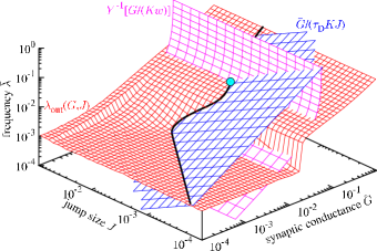
Figure 5: Extended space of Fig. 1 when the fluctuation in synaptic conductance $G$ is considered (represented by the jump size $J$). The extended neuron response function (38), the synapse response function $Y\left(\bar{\lambda}\right)=\bar{G}/\left(K\bar{w}\right)$, and the relation (39) determine the stationary states of a mean-field network (marked by a circle on the surfaces).

The process is repeated to generate the surface

$$\bar{\lambda}=\lambda_{\mathrm{out}}\left(\bar{G},J\right)$$ (38)

as plotted in Fig. 5; compare to the line representing $\lambda\left(G\right)$ as plotted in Fig. 1. The jump size $J$ is an estimator of the fluctuations in the total synaptic conductance $G\left(t\right)$, and in the $J=0$ limit, the two-parameter response function $\lambda_{\mathrm{out}}\left(\bar{G},\lambda\right)$ reduces to the single parameter response function $\lambda_{\mathrm{out}}\left(\bar{G},0\right)=\lambda\left(\bar{G}\right)$.

As we are considering a mean-field network with $K$ afferent synapses per neuron, the total frequency of presynaptic events for a postsynaptic neuron is given by $\lambda_{\mathrm{total}}=K\bar{\lambda}$, where $\bar{\lambda}$ is the mean-field firing frequency for any neuron. Combining with the relation (37), this gives us the condition

$$\frac{\bar{G}}{K\tau_{D}J}=\bar{\lambda},$$ (39)

as plotted in Fig. 5, forming a planar surface in the logarithmic-scale $\bar{G}$–$J$–$\bar{\lambda}$ space.

Whatever the value of $J$, the synaptic response function $Y\left(\bar{\lambda}\right)$ determines the mean total synaptic conductance $\bar{G}=K\bar{w}Y\left(\bar{\lambda}\right)$ when $\bar{\lambda}$ is given for the mean-field network. The inverse

$$\bar{\lambda}=Y^{-1}\left(\frac{\bar{G}}{K\bar{w}}\right),$$ (40)

also plotted in Fig. 5 with Eq. (19), represents the convex surface invariant along the $J$-axis. Along with the surfaces (38) and (39), the intersections of the three surfaces determine the fixed points of the system (marked with a circle in Fig. 5). While the neuron response function $\lambda_{\mathrm{out}}\left(\bar{G},J\right)$ is evaluated numerically, we determine the fixed points in the mean-field firing frequency numerically from the intersections of the three surfaces in Fig. 5, varying the mean synaptic weight $\bar{w}$ for a given number of afferent synapses $K$ per neuron.

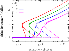
Figure 6: Numerical mean-field phase diagram (firing frequency $\bar{\lambda}$ versus synaptic weight $\bar{w}$) for various numbers $K$ (as labeled in legend) of afferent synapses per neuron under fluctuating total synaptic conductance (drawn lines) compared with the analytical results when the total synaptic conductance $G=\bar{G}$ is assumed to be constant (dashed line).

The resulting phase diagram is plotted in Fig. 6 for various $K$ values. The hysteresis vanishes at $K=K_{C}\approx 10$, and the transition from noise dominance to persistent activity becomes continuous. In our case, the fluctuation comes from the fact that the number of afferent synapses is finite. We expect that, in a real biological network, other sources of fluctuations can play a similar role to smooth out the first-order phase transition separating a noise dominated regime from persistent activity as predicted by the analytical mean-field theory of Section III.

V.2 Correction to synaptic weight distribution

Besides smoothing out the first-order phase transition in a mean-field network, the fluctuation in total synaptic conductance can also influence the stationary distribution of synaptic weights. We have noted that the width of the synaptic weight distribution predicted by the simplest mean-field approach (about 1% of $w^{\star}$) is too small in comparison with results of simulations on fully connected plastic integrate-and-fire networks (about 5% of $w^{\star}$ Chen and Jasnow ). One of the approximations we made in arriving at Eq. (27) is to replace the time-dependent $Y$ (or the fractions $A$ and $B$ that it represents) with its average value. Such an approximation can be improved by considering the second moment of $Y$ in deriving the diffusion coefficient $D$ in Eq. (23). We expect the fluctuation in $Y$ to be important when the mean-field firing frequency is low. In this limit the time-dependent $Y\left(t\right)$ is a sum of pulses

$$Y\left(t\right)=u\sum_{i}\theta\left(t-t_{i}\right)e^{-\left(t-t_{i}\right)/\tau_{D}},$$ (41)

where $\theta\left(t\right)$ is a step function with $\theta\left(t\geq 0\right)=1$ and $\theta\left(t<0\right)=0$, $\{t_{i}\}$ are the firing times of the neuron, and mean $\left\langle Y\right\rangle=u\tau_{D}\lambda$. When the overlap of the pulses can be ignored, for example, in the noise dominated regime, the mean square of $Y$ is given by $\left\langle Y^{2}\right\rangle=u^{2}\tau_{D}\lambda/2$, which should replace the squares of $Y$ in the diffusion coefficient (23). This leads to a width of the synaptic weight distribution of

$$\Delta w\simeq\sqrt{r\frac{\left\langle Y^{2}\right\rangle}{\bar{Y}}}w^{\star}=\sqrt{ur/2}w^{\star}$$ (42)

instead of Eq. (28). For the values of the parameters we have considered, this represents about 5% of $w^{\star}$ and is similar to the simulation results from a fully connected network Chen and Jasnow in the noise-dominated regime. We have verified the analytical result (42) through numerical simulations of a random walk process for the synaptic weight described by the dynamics (11).

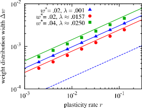
Figure 7: Numerical results (symbols) for the width of synaptic-weight distribution, $\Delta w$, as a function of plasticity rate, $r$, in a limited system of a single synapse between two neurons with Poisson spike trains following the dynamics (11) and operating at three of the fixed points predicted by the mean-field theory (as marked by corresponding symbols in Fig. 2). The results are compared with the analytical predictions (lines of corresponding colors) from Eq. (42) (drawn lines) and Eq. (28) (dashed line).

As shown in Fig. 7, the scaling in plasticity rate $r$ continues to be described by $\Delta w\sim r^{\alpha}$ with $\alpha\simeq 1/2$ in all cases, while the amplitudes match well for the noise-dominated fixed point but show small deviations when the system is persistently active. In general, we can expect fluctuations to play an important role in determining the synaptic weight distribution of a plastic network. Here we have shown that a significant correction can be accounted for by considering the fluctuation in the neural transmission for a limited system of a single synapse between two neurons with Poisson spike trains. Even without an analytical solution, such a system can be easily simulated to any desirable accuracy to obtain the stationary synaptic weight distribution as well as the average synaptic weight $\left\langle w\right\rangle$, which provides the self-consistency condition (21) for the mean-field theory.

Here we have preserved the basic structure of the mean-field approach under the additional consideration of fluctuations in synaptic conductance by extending the neuron and synapse response functions to functions of two variables. The additional degree of freedom, the average jump size $J$ of active transmitter fractions, was fixed by the condition (39) coming from the nature of such a fluctuation and does not enter the final result (42) explicitly.

VI Summary and conclusion

Models of plastic neural networks can generally be broken down into three parts: (i) the modeling of the dynamics of the neuron state (represented by the membrane potential), (ii) the modeling of synaptic transmission, and (iii) the plasticity rules. We have applied a mean-field theory that follows this basic structure. In the mean-field framework of the current study, we reduce the dynamics of the neuron state to a response function $\lambda\left(G\right)$ representing the mean firing frequency of a neuron when it is driven by a constant total synaptic conductance $G$. Similarly, the dynamics of synaptic transmission is also reduced to a characteristic response function $Y\left(\lambda\right)$ representing the mean fraction of active neural transmitter given the Poisson firing frequency $\lambda$ of the presynaptic neuron. With the mean-field synaptic weight $\bar{w}$ of a network with $K$ afferent synapses per neuron and the mean-field firing frequency $\bar{\lambda}$, the average total synaptic conductance is given by $\bar{G}=K\bar{w}Y\left(\bar{\lambda}\right)$. This allows one to plot the synapse response function $Y\left(\lambda\right)$ along with the neuron response function $\lambda\left(G\right)$ (see Fig. 1) to determine self-consistently the mean-field firing frequency $\bar{\lambda}$ as a function of $\bar{w}$ and $K$.

The mean-field firing frequency $\bar{\lambda}$ and the mean synaptic weight $\bar{w}$ characterize the mean-field network completely. We then use this mean-field network as an environment and investigate the dynamics of spike-timing-dependent plasticity (8) of a single synapse in such an environment. Assuming Poisson statistics for the spike trains, the dynamics (8) can be viewed as describing a type of random walk in synaptic weight space, where the frequency of potentiation and the jump size of depression are dependent on the weight of this synapse. The distribution of synaptic weights can be calculated numerically for the stationary state using straightforward simulations of the single synapse system. Under the approximation of small jumps, the stationary distribution can be calculated analytically from the Fokker–Planck equation arising from the master equation. The self-consistency of the mean-field approach is completed by requiring that the mean of the synaptic weight distribution $\left\langle w\right\rangle$ reproduces the mean-field synaptic weight $\bar{w}$ of the environment.

We have considered a network of integrate-and-fire neurons Dayan and Abbott (2001) coupled through synapses with TUM dynamics Tsodyks et al. (2000) within the mean-field framework outlined above. We chose integrate-and-fire neurons for their simplicity and wide use. We chose the TUM model of neural transmission for its features and flexibility as noted above. On the simplest level for a static network, our mean-field approach amounts to finding intersects of the neuron response function and synapse response function, each of which can be calculated separately from the particular neuron model and synapse model selected. Our choice of model happens to allow us to find analytical forms of the mean-field response functions for the neurons and synapses, and predict a first-order phase transition from a noise-dominated regime to a regime of persistent activity as the mean-field synaptic weight is increased. (However, see below.) In general, these response functions can be computed numerically in a straightforward fashion for a variety of neuron and synapse models regardless of the number of empirical parameters they might carry. In Fig. 1, we showed the results of such calculation for the Morris–Lecar neuron used in Volman et al. (2007) which was defined by more than twenty parameters.

For the dynamics of the synaptic weight, for specificity, we follow the spike-timing-dependent plasticity rules proposed by van Rossum, Bi, and Turrigiano van Rossum et al. (2000), with additive potentiation and multiplicative depression. The Fokker–Planck analysis of the corresponding random walk process predicts a narrow Gaussian distribution for the synaptic weight centered around $w^{\star}$, the control parameter (12) entering the plasticity rules. [See, e.g., Eq. (11).] We apply a small perturbation to the $\left\langle w\right\rangle=\bar{w}=w^{\star}$ solution, analyze its stability analytically and numerically, and find it to be stable for any number of afferent synapse per neuron $K\geq 1$ for the model and parameter ranges we considered. However, the analytical expression (35) for the stability, which is generic for any neuron and synapse response functions, also suggests that for models in which the neuron firing rate $\lambda\left(G\right)$ saturates for large conductance $G$ (for example, models with a refractory period for the firing of neurons) or where the synapse response function $Y\left(\lambda\right)$ does not saturate for large $\lambda$, (for example, when the effect of presynaptic firings is additive and $Y$ no longer represents a fraction), the fixed point $\bar{w}=w^{\star}$ can not remain stable for large $w^{\star}$. It is then possible to have runaway or pile-up in the resulting synaptic weight distribution.

For a network of finite $K$ and low overall frequency $\lambda_{\mathrm{total}}$ of presynaptic events, the “shot noise” due to the discrete nature of presynaptic spikes is not negligible, and one at least needs to expand the description of the mean-field response of a neuron to include temporal fluctuations. We have done this approximately via a two-variable function, e.g., $\lambda_{\mathrm{out}}\left(\bar{G},J\right)$, where $J$, representing fluctuations, describes the size of the jumps in a neuron’s total synaptic conductance for each presynaptic event. We evaluate this two-variable response function numerically for a single neuron, modeling its total synaptic conductance with a simple stochastic jump-and-decay process (36). The results suggest the disappearance of the first-order transition when the number, $K$, of afferent synapses per neuron is less than a critical value $K_{C}\approx 10$. In realistic situations fluctuations can be expected to smear out the first-order transition. When a corresponding fluctuation is considered for the variable $Y$ governing jump sizes in the plasticity rules (11), the Fokker–Planck approach predicts a broader Gaussian distribution which has a width similar to the observed width in full network simulations Chen and Jasnow . The results of extensive simulations on a fully connected plastic network will be published elsewhere.

The inclusion of fluctuations at some level, such as within our extended mean-field theory (see Sec. V), hints at a possible critical state of the system at the endpoint of a first-order transition line in analogy with the vapor pressure curve of a fluid, see, e.g., Huang (1988). While criticality in neural avalanches has been observed by Beggs and Plenz Beggs and Plenz (2003), within the extended mean-field analysis employed in the current study the system does not appear to organize into such a critical state without a requisite tuning of the fluctuation-amplitude and perhaps plasticity parameters, e.g., $w^{\star}$. This is in contrast with the suggestion that such criticality should be self-organized Beggs and Plenz (2003); Chialvo (2004). It thus will be of great interest to find missing elements, possibly in the plasticity rules, that could dynamically push the network close to a critical state. Along this direction, one can expect a variety of model candidates, which can be easily subjected to the type of mean-field scheme outlined in the current study to provide additional qualitative and semi-quantitative insight into their plausibility. We also note in passing that “all-to-all” network simulations using the plasticity rules and neuron modeling described in this paper have not revealed evidence for a self-organized critical state. In that regard, sparse networks would appear to be better suited, but mean-field analysis such as presented here will mainly have only qualitative use. Our simulations of integrate-and-fire and other neuronal networks with the plasticity rules used here will be presented elsewhere.

As noted in the Introduction, the current study cannot begin to address how brains function or form. As a real brain is never uniform or stationary, we do not expect the model systems presented here to address or reproduce its dynamics. However, there are cultured networks consisting of hundreds of neurons with virtually “all-to-all” interactions Bi and Poo (1998); Segev et al. (2001); Shefi et al. (2002); Beggs and Plenz (2003); Lai et al. (2006). The studies of these networks in vitro is an important steppingstone towards the understanding of more complicated networks. The dynamics of these cultured network are on a scale very much accessible to current neural network modeling, such as the one presented here, and simulation, as noted, to be presented elsewhere.