THE COSMIC NEAR INFRARED BACKGROUND II: FLUCTUATIONS

Abstract

The Near Infrared Background (NIRB) is one of a few methods that can be used to observe the redshifted light from early stars at a redshift of six and above, and thus it is imperative to understand the significance of any detection or non-detection of the NIRB. Fluctuations of the NIRB can provide information on the first structures, such as halos and their surrounding ionized regions in the Inter Galactic Medium (IGM). We combine, for the first time, $N$-body simulations, radiative transfer code, and analytic calculations of luminosity of early structures to predict the angular power spectrum ($C_{l}$) of fluctuations in the NIRB. We study, in detail, the effects of various assumptions about the stellar mass, the initial mass spectrum of stars, metallicity, the star formation efficiency ($f_{*}$), the escape fraction of ionizing photons ($f_{\rm esc}$), and the star formation timescale ($t_{\rm SF}$), on the amplitude as well as the shape of $C_{l}$. The power spectrum of NIRB fluctuations is maximized when $f_{*}$ is the largest (as $C_{l}\propto f_{*}^{2}$) and $f_{\rm esc}$ is the smallest (as more nebular emission is produced within halos). A significant uncertainty in the predicted amplitude of $C_{l}$ exists due to our lack of knowledge of $t_{\rm SF}$ of these early populations of galaxies, which is equivalent to our lack of knowledge of the mass-to-light ratio of these sources. We do not see a turnover in the NIRB angular power spectrum of the halo contribution, which was claimed to exist in the literature, and explain this as the effect of high levels of non-linear bias that was ignored in the previous calculations. This is partly due to our choice of the minimum mass of halos contributing to NIRB ($\sim 2\times 10^{9}~{}M_{\sun}$), and a smaller minimum mass, which has a smaller non-linear bias, may still exhibit a turn over. Therefore, our results suggest that both the amplitude and shape of the NIRB power spectrum provide important information regarding the nature of sources contributing to the cosmic reionization. The angular power spectrum of the IGM, in most cases, is much smaller than the halo angular power spectrum, except when $f_{\rm esc}$ is close to unity, $t_{\rm SF}$ is longer, or the minimum redshift at which the star formation is occurring is high. In addition, low levels of the observed mean background intensity tend to rule out high values of $f_{*}\gtrsim 0.2$.

1 INTRODUCTION

We have few probes of the early universe and the first few generations of stars. We know that stars had to form early in order to pollute the universe with metals and reionize the universe. There is evidence that the universe was reionized at around $z\sim 11$, such as from the Wilkinson Microwave Anisotropy Probe (WMAP) satellite (Kogut et al., 2003; Spergel et al., 2003, 2007; Page et al., 2007; Dunkley et al., 2009; Komatsu et al., 2009). Stars are efficient producers of ionizing photons, so are likely candidates for the bulk of reionization. These ultraviolet photons at redshifts $6\lesssim z\lesssim 30$ would be redshifted into the near-infrared bands. Therefore, it makes sense to search for this remnant light in the near infrared bands to learn about this early epoch of star formation and reionization (Santos, Bromm & Kamionkowski, 2002; Magliocchetti, Salvaterra, & Ferrara, 2003; Salvaterra & Ferrara, 2003; Cooray et al., 2004; Cooray & Yoshida, 2004; Kashlinsky et al., 2004; Madau & Silk, 2005; Fernandez & Komatsu, 2006). Observations of the Near Infrared Background (NIRB) may indicate that there is an excess mean background above that normal galaxies can account for (Dwek & Arendt, 1998; Gorjian, Wright & Chary, 2000; Kashlinsky & Odenwald, 2000; Wright & Reese, 2000; Wright, 2001; Cambresy et al., 2001; Totani et al., 2001; Matsumoto et al., 2005; Kashlinsky, 2005). In addition, there also appears to be a peak in the NIRB spectrum at 1–2 $\mu{\rm m}$, which could represent a Lyman-cutoff signature (Bock et al., 2006). However, the interpretation of the current observational data, in particular accuracy of the subtraction of Zodiacal light and foreground galaxies, is highly controversial (Thompson et al., 2007a, b). Nevertheless, any detection or non-detection of this excess light could tell us properties of early stars.

In addition to the mean intensity, fluctuations in the NIRB can provide an additional source of information about the first generations of stars (Kashlinsky & Odenwald, 2000; Kashlinsky et al., 2002, 2004, 2005, 2007a, 2007b, 2007c; Kashlinsky, 2005; Magliocchetti, Salvaterra, & Ferrara, 2003; Odenwald et al., 2003; Cooray et al., 2004; Matsumoto et al., 2005; Thompson et al., 2007a, b). Fluctuations are in general easier to study than the mean intensity because an accurate determination of the zero point is not needed; thus, they are less sensitive to the imperfect subtraction of Zodiacal light. However, as the contribution to fluctuations from low redshift populations, i.e., $z<6$, can confuse the signal from higher redshift populations, the level of contamination from low redshift populations must be estimated and subtracted carefully (Sullivan et al., 2007; Cooray et al., 2007; Kashlinsky et al., 2007c; Thompson et al., 2007b; Chary, Cooray & Sullivan, 2008). Upcoming measurements with AKARI (Matsuhara et al., 2008) and CIBER (the Cosmic Infrared Background Experiment) (Bock et al., 2006; Cooray et al., 2009) may be able to put a more solid constraint on what fraction of the NIRB is from high redshift stars and galaxies.

In the previous paper we have presented detailed theoretical calculations of the spectrum and metallicity/initial-mass-spectrum dependence of the mean intensity of NIRB (Fernandez & Komatsu (2006), hereafter FK06). In this paper we present calculations of the power spectrum and metallicity/initial-mass-spectrum dependence of the NIRB fluctuations, as well as dependence on the star formation efficiency and the escape fraction of ionizing photons. While the previous work in the literature (Cooray et al., 2004; Kashlinsky et al., 2004) relied solely on simplified analytical arguments, we use, for the first time, large-scale cosmological simulations of cosmic reionization given in Iliev et al. (2006, 2007, 2008b), coupled with the analytical calculations given in FK06, to predict the power spectrum of NIRB fluctuations. In this way we are able to capture the contribution from ionized bubbles surrounding the halos, which has been ignored completely in the previous work.

In § 2 we outline the simulations (Iliev et al., 2006, 2007, 2008b) and in § 3 we explain the analytic formulas we use to obtain the luminosity of the halos and the surrounding IGM. In § 4 we present our calculation of the luminosity-density power spectrum, $P_{L}(k)$. Predictions for $P_{L}(k)$ and the angular power spectrum of NIRB fluctuations, $C_{l}$, are presented in § 5. Various parameters’ effects on the results are discussed in § 6. We compare our results to the previous literature in § 7 and to observations in § 8. We take a look at the constraints from the mean NIRB in § 9, and compute the fractional anisotropy, i.e., the ratio of the power spectrum and the mean intensity squared, in § 10. We conclude in § 11.

2 SIMULATION

We use simulations from Iliev et al. (2006, 2007, 2008b), which are the first truly large scale simulations to include radiative transfer, and are therefore ideal for predicting the distribution of luminosities from high redshift stellar populations. Simulations provide the advantage of being able to simultaneously model the distribution of halos and the density of the IGM, as well as the ionization front that propagates through the IGM. We combine this $N$-body code with radiative transfer and analytic formulas for luminosity to simulate their luminosity-density power spectrum.

The particular simulation that we use in this paper is the run “f250C” in Table I of Iliev et al. (2008b), which was run with the cosmological parameters given by the WMAP 3-year results (Spergel et al., 2007), ($\Omega_{\rm m}$, $\Omega_{\Lambda}$, $\Omega_{\rm b}$, $h$, $\sigma_{8}$, $n_{\rm s}$)=(0.24, 0.76, 0.042, 0.73, 0.74, 0.95). Aside from the cosmological parameters, the only free parameter in the reionization simulation of this kind is the production rate of ionizing photons escaping into the IGM per halo. We shall come back to this parameter, called $f_{\gamma}/t_{\rm SF}$, in § 3.2.

These simulations combine a high resolution $N$-body code (PMFAST, see Merz, Pen & Trac, 2005) with a radiative transfer code ($C^{2}$-Ray, see Mellema et al., 2006), which is a conservative, causal ray-tracing radiative transfer code. The $C^{2}$-Ray code traces the ionization front by tracking photons using photon conservation. The code allows for large time steps and coarse grids without loss of accuracy.

The box size of the simulation is 100$~{}h^{-1}$ Mpc, which is large enough to sample the history, geometry, and statistical properties of reionization. The number of particles is $1624^{3}$, and the density field was sampled on a lattice of $3248^{3}$ cells. The density field was then binned to $203^{3}$ cells for the radiative transfer calculations. We use the $203^{3}$ cells when we compute the radiation from the IGM in § 4.2. The minimum mass of the halos is $2.2\times 10^{9}~{}M_{\sun}$, which represents dwarf galaxies. These halos have virial temperatures of $1.2\times 10^{4}\>{\rm K}$, $1.8\times 10^{4}\>{\rm K}$, and $2.6\times 10^{4}\>{\rm K}$ at $z=6$, $10$, and $15$ respectively. For these halos the dominant cooling process is hydrogen atomic cooling. It is important to sample these dwarf galaxies, as they are far more numerous than larger galaxies and may provide most of the photons needed for reionization.

Even though this simulation is a very powerful tool, it is important to consider its limitations. Halos slightly below the resolution of this simulation ($10^{8}$ to $10^{9}~{}$ $M_{\sun}$) may also be an important source for ionizing radiation. Iliev et al. (2007) also did a smaller box-size simulation [(35$~{}h^{-1}$ Mpc)³] that resolves halos down to $10^{8}~{}M_{\sun}$, which includes halos that form stars as a result of atomic cooling. These smaller halos allow the ionization fraction to reach 50% at an earlier epoch than the simulations that only resolved down to $2.2\times 10^{9}~{}M_{\sun}$. However, Iliev et al. (2007) found that the redshift in which reionization was completed remained about the same for the 100$~{}h^{-1}$ Mpc and 35$~{}h^{-1}$ Mpc simulations, due to the “self-regulation” (see Iliev et al., 2007, for details).

The results discussed in this paper are based on the larger box size with halos resolved down to $2.2\times 10^{9}~{}M_{\sun}$. It is possible that the smaller halos would affect the fluctuations in the NIRB from both the halos and the IGM. Future simulations will allow both a larger box size along with a smaller minimum mass. These future simulations will be able to provide more robust predictions for the fluctuations in the NIRB if these smaller halos contribute to the NIRB. Simulations that resolve halos smaller than $10^{8}~{}M_{\sun}$ may not be needed, however: while these minihalos were likely the sites of the truly first generation of stars, they may not be a significant source of ionizing photons to reionize the universe, as UV photons in the Lyman Werner bands dissociate molecular hydrogen, terminating star formation in these small halos (Haiman, Rees & Loeb, 1997; Haiman, Abel & Rees, 2000; Machacek, Bryan & Abel, 2003; Yoshida et al., 2003; Johnson, Grief & Bromm, 2008; Ahn et al., 2009). However, there is on-going discussion as to what the radiation feedback actually does for the formation of second generation stars (Wise et al., 2007; Ahn & Shapiro, 2007; O’Shea & Norman, 2008). While the Lyman Werner background from early star formation has a primarily negative feedback effect, other processes (e.g., cooling in supernova remnant shocks) may mitigate the suppression of H2 molecules (Ferrara, 1998; Ricotti et al., 2001).

3 ANALYTICAL CALCULATION

In this section we describe how we assign the luminosity to the halos and the IGM in the simulation. Note that our method is fully analytical, and thus can be adopted to any other reionization simulations.

3.1 Luminosity of the halos

Luminosity within the halos is dominated by five radiative processes: stellar (black-body) emission, and the nebular emission including free-free, free-bound, and two-photon emission, as well as any emission lines (here, Lyman-$\alpha$ is the most important one for our study of NIRB). The luminosity of each component can be found analytically using the equations in FK06. Equations for the stars’ luminosity, temperature, number of ionizing photons per second, and lifetime were based on equations from Table 3 of Fernandez & Komatsu (2008), which were fit from stellar models or fitting functions (Marigo et al., 2001; Lejeune & Schaerer, 2001; Schaerer, 2002).

First, let us define the “volume emissivity.” The volume emissivity (luminosity per comoving volume per frequency), $p(\nu)$, is related to the “emission coefficient” (luminosity per comoving volume per frequency per steradian), $j_{\nu}$, in Santos, Bromm & Kamionkowski (2002); Cooray et al. (2004) by $p(\nu)=4\pi j_{\nu}$. In other words, the luminosity is given by

$$dL=p(\nu)d\nu dV=j_{\nu}d\Omega d\nu dV,$$ (1)

where $dV$ is the comoving volume element, and $d\Omega$ is the solid angle element. Integrating $p(\nu)$ over $\nu$, one obtains the “comoving luminosity density,” $\rho_{L}$, as $dL=\rho_{L}dV$, where $\rho_{L}=\int p(\nu)d\nu$.

When the main-sequence lifetime of stars under consideration is shorter than the time scale at which the star formation takes place, the volume emissivity is given by a product of the star formation rate (the stellar mass density formed per unit time), $\dot{\rho}_{*}(z)$, and the ratio of the mass-weighted average of the total radiative energy (including stellar emission and reprocessed light) emitted over the stellar lifetime to the stellar rest-mass energy, $\langle\epsilon_{\nu}^{\alpha}\rangle$ (see Eq. (2) of FK06):

$$p(\nu,z)=\sum_{\alpha}p_{\alpha}(\nu,z)=\dot{\rho}_{*}(z)c^{2}\sum_{\alpha}\langle\epsilon^{\alpha}_{\nu}\rangle,$$ (2)

where

$$\langle\epsilon_{\nu}^{\alpha}\rangle=\frac{\int^{m_{2}}_{m_{1}}dm\left[L^{\alpha}_{\nu}(m)\tau(m)/(mc^{2})\right]f(m)m}{\int^{m_{2}}_{m_{1}}dmf(m)m}.$$ (3)

Here, $m$ is the stellar mass, $L_{\nu}^{\alpha}(m)$ is the time-averaged luminosity per frequency of a given radiative process $\alpha$ (which includes the stellar, free-free, free-bound, two-photon, and Lyman-$\alpha$ emission), $\tau(m)$ is the main sequence lifetime, and $f(m)$ is the initial mass spectrum of stars under consideration (specified later in § 3.2). Note that $\langle\epsilon_{\nu}^{\alpha}\rangle$ may also be interpreted as a ratio of the total radiative energy within a unit frequency to the total stellar rest-mass energy,

$$\langle\epsilon_{\nu}^{\alpha}\rangle=\frac{\int^{m_{2}}_{m_{1}}dmf(m)L^{\alpha}_{\nu}(m)\tau(m)}{\int^{m_{2}}_{m_{1}}dmf(m)mc^{2}}.$$ (4)

Either way, $\langle\epsilon_{\nu}^{\alpha}\rangle$ is a convenient quantity that tells us how much of the stellar rest-mass energy is converted into the radiative energy within a unit frequency interval.

In FK06 we have shown that $\langle\epsilon_{\nu}^{\alpha}\rangle$ can be calculated robustly for a given stellar population, i.e., $f(m)$, using the basic stellar physics and radiative processes in the interstellar medium. For the radiative processes and stellar populations we consider in this paper, $\nu\langle\epsilon_{\nu}^{\alpha}\rangle\lesssim 10^{-3}$ (see Figure 2 of FK06). From this one may obtain a quantity that is commonly used in the literature, the luminosity per stellar mass, ${l}^{\alpha}_{\nu}$, as

$$l^{\alpha}_{\nu}(z)=\frac{p_{\alpha}(\nu,z)}{\rho_{*}(z)}=\frac{d\ln\rho_{*}(z)}{dt}\frac{\int^{m_{2}}_{m_{1}}dmf(m)L^{\alpha}_{\nu}(m)\tau(m)}{\int^{m_{2}}_{m_{1}}dmf(m)m}.$$ (5)

In this expression one may identify $d\ln\rho_{*}(z)/dt$ as the inverse of the star formation timescale, $t_{\rm SF}(z)$, i.e., $t_{\rm SF}(z)\equiv[d\ln\rho_{*}(z)/dt]^{-1}$. Therefore, we finally obtain

$$l^{\alpha}_{\nu}(z)=\frac{1}{t_{\rm SF}(z)}\frac{\int^{m_{2}}_{m_{1}}dmf(m)L^{\alpha}_{\nu}(m)\tau(m)}{\int^{m_{2}}_{m_{1}}dmf(m)m},$$ (6)

when the main sequence lifetime of stars is shorter than the star formation timescale, $\tau(m)<t_{\rm SF}(z)$. In terms of $\langle\epsilon_{\nu}^{\alpha}\rangle$ we may also write Eq. (6) as $l^{\alpha}_{\nu}(z)=\langle\epsilon_{\nu}^{\alpha}\rangle c^{2}/t_{\rm SF}(z)$.

On the other hand, when the star formation timescale is shorter than the main sequence lifetime of stars, $t_{\rm SF}(z)<\tau(m)$, we find a different expression for $l^{\alpha}_{\nu}$ (see Eq. (A6) of FK06):

$$l^{\alpha}_{\nu}=\frac{\int^{m_{2}}_{m_{1}}dmf(m)L^{\alpha}_{\nu}(m)}{\int^{m_{2}}_{m_{1}}dmf(m)m},$$ (7)

and $l^{\alpha}_{\nu}$ no longer depends on $z$ as long as $f(m)$ does not depend on $z$. From Eqs. (6) and (7) we find that the former is roughly $\tau/t_{\rm SF}$ times the latter. In other words, if one misused the latter form when $\tau<t_{\rm SF}$, one would over-estimate the signal by a factor of $\approx t_{\rm SF}/\tau$, which can be as large as a factor of 10 for short-lived, massive stars with $\sim 100~{}M_{\sun}$.

For the precise calculation one should use both expressions depending on the situation; however, to simplify the analysis, we shall use either Eq. (6) or (7), depending on the ratio of the stellar lifetime averaged over the initial mass spectrum and weighted by the luminosity (since more massive, shorter lived stars will contribute more to the overall luminosity), $\langle{\tau}\rangle\equiv\int_{m_{1}}^{m_{2}}dmf(m)\tau(m)L/\int_{m_{1}}^{m_{2}}dmf(m)L$, to the star formation timescale (where $L$ is the bolometric luminosity). In the simulations of Iliev et al. (2006, 2007, 2008b), the star formation timescale takes on a universal value, $t_{\rm SF}\approx 20$ Myr. For all the stellar populations, the luminosity-weighted lifetime is shorter than $20$ Myr; thus, Eq. 7 will be our fiducial formula.

To compute $l_{\nu}^{\alpha}$ for each radiative process, we use a black-body for the stellar component, $l^{*}_{\nu}$ (see Eq. (6) of FK06). This emission is cutoff above 13.6 eV, so all of the ionizing photons go into producing emission in the nebula or the IGM. The expressions given in § 2.3, 2.4, and 2.5 of FK06 are used for the nebular processes. We then integrate $l^{\alpha}_{\nu}$ over a band of observed frequencies $\nu_{1}$ to $\nu_{2}$ to obtain the band-averaged luminosity per stellar mass, $\bar{l}^{\alpha}$, as

$$\bar{l}^{\alpha}(z)\equiv\int^{\nu_{2}(1+z)}_{\nu_{1}(1+z)}d\nu~{}l^{\alpha}_{\nu}(z).$$ (8)

Following Iliev et al. (2006, 2007, 2008b), we assume all halos have a constant mass-to-light ratio. With the luminosities per stellar mass, $\bar{l}^{\alpha}(z)$, computed, we obtain the luminosities of the halo, $L_{h}(z)$, by multiplying $\bar{l}(z)$ by the total stellar mass per halo, $f_{*}M_{h}(\Omega_{b}/\Omega_{m})$, where $M_{h}$ is the total halo mass (including dark matter and baryons), and $f_{*}$ is the star formation efficiency, which is the fraction of baryons that can form into stars over the star formation timescale $t_{\rm SF}$. We find

$$\frac{L_{h}(z)}{M_{h}}=f_{*}\frac{\Omega_{b}}{\Omega_{m}}\left\{\bar{l}^{*}(z)+(1-f_{\rm esc})\left[\bar{l}^{ff}(z)+\bar{l}^{fb}(z)+\bar{l}^{2\gamma}(z)+\bar{l}^{\rm Ly\alpha}(z)\right]\right\},$$ (9)

where $f_{\rm esc}$ is the escape fraction of ionizing photons from the halo. Only those photons that do not escape into the IGM produce nebular emission within the halo.

From this result one may conclude immediately that the NIRB power spectrum from halos, which is proportional to $(L_{h}/M_{h})^{2}$, is proportional to $f_{*}^{2}$. Also, $L_{h}/M_{h}$ goes down as $f_{\rm esc}$ approaches unity, for which all the ionizing photons would escape halos, and thus no nebular emission would be left in halos. The stellar properties, such as metallicities and initial mass spectra, affect only $\bar{l}^{\alpha}$.

3.2 Stellar Populations

The simulations from Iliev et al. (2008b) define a quantity, $f_{\gamma}$, which is proportional to the number of ionizing photons that escape into the IGM:

$$f_{\gamma}=f_{*}f_{\rm esc}N_{i},$$ (10)

where $N_{i}$ is the number of ionizing photons emitted per stellar atom. When modeling stellar populations in our calculations, we shall assure that each of our models agrees with $f_{\gamma}=250$, which was used in the simulations.

Iliev et al. (2008b) have shown that this choice of $f_{\gamma}$, combined with the universal star formation timescale of $t_{\rm SF}=20~{}{\rm Myr}$, can reionize the universe successfully with the resulting electron-scattering optical depth consistent with the WMAP data. Within this framework, since $f_{\gamma}/t_{\rm SF}$ is the only free parameter, models with the same $f_{\gamma}/t_{\rm SF}$ would produce the same reionization histories. (For the simulation case f250C on which our calculations here are based, for example, the globally-averaged ionized fraction of the IGM was found to be 50% at $z=8.3$ and 99% at $z=6.6$.) To keep $f_{\gamma}/t_{\rm SF}$ constant, the star formation efficiency must decrease as the escape fraction increases. The various populations that were modeled are shown in Table 1.

Population	Initial Mass Spectrum	$m_{1},m_{2}$	$\langle\tau\rangle$ (Myr)	$N_{i}$	$f_{\rm esc}$	$f_{*}$
Pop III	Salpeter	$3M_{\sun}$, $150M_{\sun}$	8.08	5600	0.22	0.2
Pop III	Larson, $m_{c}=250M_{\sun}$	$3M_{\sun}$, $500M_{\sun}$	2.45	25000	0.1	0.1
Pop III	Salpeter	$3M_{\sun}$, $150M_{\sun}$	8.08	5600	0.9	0.05
Pop III	Larson, $m_{c}=250M_{\sun}$	$3M_{\sun}$, $500M_{\sun}$	2.45	25000	1	0.01
Pop II	Salpeter	$3M_{\sun}$, $150M_{\sun}$	9.04	2600	0.95	0.1
Pop II	Larson, $m_{c}=50M_{\sun}$	$3M_{\sun}$, $150M_{\sun}$	4.87	12000	0.9	0.023
Pop II	Salpeter	$3M_{\sun}$, $150M_{\sun}$	9.04	2600	0.19	0.5
Pop II	Larson, $m_{c}=50M_{\sun}$	$3M_{\sun}$, $150M_{\sun}$	4.87	12000	0.098	0.21

Table 1: Stellar populations (“Pop III” are metal-free, and “Pop II” are metal-poor with the metallicity of $Z=1/50~{}Z_{\sun}$), parameters for initial mass spectra, the luminosity-weighted main sequence lifetime of stars ($\langle\tau\rangle$), the corresponding number of ionizing photons per stellar atom ($N_{i}$), escape fractions of ionizing photons ($f_{\rm esc}$), and the star formation efficiency ($f_{*}$). Note that $f_{\rm esc}$ and $f_{*}$ are tuned such that the value of $f_{\gamma}=f_{\rm esc}f_{*}N_{i}$ is held fixed at $f_{\gamma}=250$ which, when combined with the star formation timescale of $t_{\rm SF}=20~{}{\rm Myr}$, can reionize the universe such that the resulting electron-scattering optical depth is consistent with the WMAP data.

We modeled both zero metallicity stars (Population III; $Z=0$) and low metallicity stars (Population II; $Z=1/50~{}Z_{\sun}$) with either a heavy or a light initial mass spectrum, accompanied with either a low escape fraction ($f_{\rm esc}\sim 0.1$) or a high escape fraction ($f_{\rm esc}\sim 1$). While we try to simulate a range of parameters, it is good to keep in mind that our choice of $f_{*}$ and $f_{\rm esc}$ for a given $f_{\gamma}$ is basically arbitrary. The level of NIRB fluctuations can change significantly when paired with different assumptions for the metallicity, mass, and values for $f_{\rm esc}$ and $f_{*}$.

A lighter mass distribution of stars is represented by a Salpeter initial mass spectrum (Salpeter, 1955)

$$f(m)\propto m^{-2.35}.$$ (11)

We use mass limits of $m_{1}=3M_{\sun}$ and $m_{2}=150M_{\sun}$ for this spectrum. Heavier stars are represented by a Larson initial mass spectrum (Larson, 1998)

$$f(m)\propto m^{-1}\left(1+\frac{m}{m_{c}}\right)^{-1.35},$$ (12)

with $m_{1}=3M_{\sun}$, $m_{2}=500M_{\sun}$, and $m_{c}=250M_{\sun}$ for Population III stars and $m_{1}=3M_{\sun}$, $m_{2}=150M_{\sun}$, and $m_{c}=50M_{\sun}$ for Population II stars.

In Figure 1 we show $\nu l^{\alpha}_{\nu}$ (in units of nW $M_{\sun}^{-1}$), and in Figure 2 we show $\bar{l}^{\alpha}(z)$ (in units of nW $M_{\sun}^{-1}$) averaged over a rectangular bandpass from $1-2~{}\mu{\rm m}$, for the stellar populations we consider in this paper. In the relevant redshift range, $7\lesssim z\lesssim 15$, the stellar, two-photon, and Ly$\alpha$ emission are the most dominant radiation processes, and all of them are on the order of $\bar{l}\sim 10^{38}~{}{\rm nW}~{}M_{\sun}^{-1}~{}(20~{}{\rm Myr}/t_{\rm SF})$.

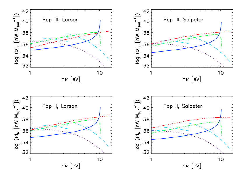
Figure 1: Luminosity spectrum per stellar mass. The stellar, $\nu l^{*}_{\nu}$ (triple-dot dashed red line), free-free, $\nu l_{\nu}^{ff}$ (dotted purple line), free-bound, $\nu l_{\nu}^{fb}$ (dashed light blue line), two-photon, $\nu l_{\nu}^{2\gamma}$ (dot dashed green line), and Lyman-$\alpha$ emission, $\nu l_{\nu}^{\rm Ly\alpha}$ (solid dark blue line), are shown in units of nW $M_{\sun}^{-1}$ as a function of the rest-frame energies. The stars are at $z=10$, but the redshift affects the profile of the Lyman-$\alpha$ line only, which was taken from Eq. (15) of Santos, Bromm & Kamionkowski (2002).

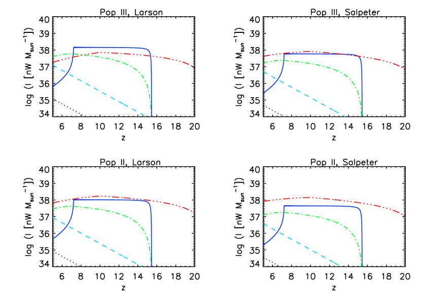
Figure 2: Luminosity per stellar mass averaged over a rectangular bandpass from $1-2~{}\mu{\rm m}$. The stellar, $\bar{l}^{*}$ (triple-dot dashed red line), free-free, $\bar{l}^{ff}$ (dotted purple line), free-bound, $\bar{l}^{fb}$ (dashed light blue line), two-photon, $\bar{l}^{2\gamma}$ (dot dashed green line), and Lyman-$\alpha$ emission, $\bar{l}^{\rm Ly\alpha}$ (solid dark blue line), are shown in units of nW $M_{\sun}^{-1}$ as a function of redshifts. Free-free and free-bound both decrease with redshift. This is because both decrease with energy, and as redshift is increased, the bandwidth corresponds to higher rest-frame energies. The initial rise in Lyman-$\alpha$ is due to the wing of the line. At $z\sim 15.5$, the line hits the end of the band where there is no more Lyman-$\alpha$ emission. Stellar emission increases initially because there is more emission from the star as energy increases, and later decreases as the bandwidth begins to sample energies above 13.6 eV. Two photon emission is cut off at $z\sim 15.5$, which corresponds to the band sampling above 10.2 eV, above which there is no emission.

3.3 Luminosity Density from IGM

Photons that do escape the halos go into producing emission in the HII region surrounding the halo in the IGM (free-free, free-bound, two photon and Lyman-$\alpha$ emission). The emission in the HII region can be found using the volume emissivity, $p({\nu})$, i.e., luminosity per comoving volume per frequency, or luminosity density per frequency (see Eq. (1) for the precise definition).

Since all of the radiative processes we discuss in this section are proportional to the number density squared, we need to be careful about the comoving versus proper quantities. The proper volume emissivity is proportional to the proper number density squared, i.e., $p_{prop}\propto n_{prop}^{2}$. As the comoving volume emissivity is $p_{com}=a^{3}p_{prop}=p_{prop}/(1+z)^{3}$ and the comoving number density is $n_{com}=a^{3}n_{prop}=n_{prop}/(1+z)^{3}$, we obtain $p_{com}\propto(1+z)^{3}n_{com}^{2}$. This factor of $(1+z)^{3}$ simply reflects the fact that the IGM was denser at higher redshift, and thus the IGM was brighter. In the following derivations $n$ always refers to the comoving number density.

For free-free and free-bound emission, the volume emissivity is

$$p_{\rm ff,fb}({\nu},z)=4\pi(1+z)^{3}n_{e}n_{p}\gamma_{\rm c}\frac{e^{-h\nu/kT_{\rm g}}}{T_{\rm g}^{1/2}},$$ (13)

where $n_{e}$ and $n_{p}$ are the comoving number density of electrons and protons respectively, $\gamma_{\rm c}$ is the continuum emission coefficient including free-free and free-bound emission:

$$\gamma_{\rm c}\equiv f_{k}\left[\overline{g}_{ff}+\sum^{\infty}_{n=2}\frac{x_{n}e^{x_{n}}}{n}g_{fb}(n)\right],$$ (14)

where $x_{n}\equiv{Ry}/(kT_{\rm g}n^{2})$, $\overline{g}_{ff}$ and $g_{bf}(n)$ are the Gaunt factors for free-free (which is thermally averaged) and free-bound emission, respectively, $f_{k}$ is the collection of physical constants which has a numerical value of $5.44\times 10^{-39}$ in cgs units, and $T_{\rm g}$ is the gas temperature, which we took to be $10^{4}$ K (see § 2.3 of FK06 for more details).

Using the charge neutrality, $n_{e}=n_{p}$, we write

$$n_{e}n_{p}=n_{e}^{2}=n_{H}^{2}X_{e}^{2},$$ (15)

where $n_{H}$ is the number density of hydrogen atoms and $X_{e}$ is the ionization fraction, both of which are given in the simulation. The volume emissivity is therefore given by

$$\frac{p_{\rm ff,fb}({\nu},z)}{n_{H}^{2}X_{e}^{2}}=4\pi(1+z)^{3}\gamma_{c}\frac{e^{-h\nu/kT_{\rm g}}}{T_{\rm g}^{1/2}}.$$ (16)

The two-photon emissivity is

$$p_{2\gamma}({\nu},z)=(1+z)^{3}\frac{2h\nu}{\nu_{\rm Ly\alpha}}P(y)(1-f_{\rm Ly\alpha})\alpha_{\rm B}n_{e}n_{p},$$ (17)

A fraction of photons that make the $2-1$ transition, $(1-f_{\rm Ly\alpha})$, go into two photon emission, while the remainder, $f_{\rm Ly\alpha}$, produce the Lyman-$\alpha$ line. The precise value of $f_{\rm Ly\alpha}$ depends slightly on the temperature of gas, and for a gas at $10^{4}$ K the value of $f_{\rm Ly\alpha}$ is 0.64 (Spitzer, 1978). Here, $\alpha_{\rm B}$ is the case B hydrogen recombination coefficient given by

$$\alpha_{\rm B}=\frac{2.06\times 10^{-11}}{T_{\rm g}^{1/2}}\phi(T_{\rm g})~{}{\rm cm^{3}~{}s^{-1}},$$ (18)

where $\phi(T_{\rm g})$ is given by Spitzer (1978). Here, $P(y)$ is the normalized probability per two photon decay that one photon is in the range $dy=d\nu/\nu_{\rm Ly\alpha}$, which can be fit as (Eq. (22) of FK06)

$$P(y)=1.307-2.627(y-0.5)^{2}+2.563(y-0.5)^{4}-51.69(y-0.5)^{6},$$ (19)

and $\nu_{\rm Ly\alpha}$ is the frequency of Lyman-$\alpha$ photons. Using $n_{H}$ and $X_{e}$, we write the emissivity as

$$\frac{p_{2\gamma}({\nu},z)}{n_{H}^{2}X_{e}^{2}}=(1+z)^{3}\frac{2h\nu}{\nu_{\rm Ly\alpha}}P(y)(1-f_{\rm Ly\alpha})\alpha_{\rm B}.$$ (20)

For Lyman-$\alpha$,

$$p_{\rm Ly\alpha}({\nu},z)=(1+z)^{3}f_{\rm Ly\alpha}h\nu_{\rm Ly\alpha}n_{e}n_{p}\alpha_{\rm B}\phi(\nu-\nu_{\rm Ly\alpha}),$$ (21)

where $\phi(\nu-\nu_{\rm Ly\alpha})$ is the line profile of the Lyman-$\alpha$ line, given in Loeb & Rybicki (1999); Santos, Bromm & Kamionkowski (2002). Using $n_{H}$ and $X_{e}$, we get

$$\frac{p_{\rm Ly\alpha}({\nu},z)}{n_{H}^{2}X_{e}^{2}}=(1+z)^{3}f_{\rm Ly\alpha}h\nu_{\rm Ly\alpha}\alpha_{\rm B}\phi(\nu-\nu_{\rm Ly\alpha}).$$ (22)

Collecting all the processes we obtain the volume emissivity of the IGM as

$$\frac{p^{\rm IGM}({\nu},z)}{n_{H}^{2}X_{e}^{2}}=(1+z)^{3}\left\{4\pi\gamma_{c}\frac{e^{-h\nu/kT_{\rm g}}}{T_{\rm g}^{1/2}}+\alpha_{\rm B}h\nu_{\rm Ly\alpha}\left[(1-f_{\rm Ly\alpha})\frac{2\nu P(\nu/\nu_{\rm Ly\alpha})}{\nu^{2}_{\rm Ly\alpha}}+f_{\rm Ly\alpha}\phi(\nu-\nu_{\rm Ly\alpha})\right]\right\}.$$ (23)

We are now in a position to find the emission of the IGM by pairing these formulas with the hydrogen number densities ($n_{H}$) and the ionization fractions ($X_{e}$) from the simulations. In Figure 3 we show $\nu p_{\alpha}(\nu,z)/[(1+z)^{3}n_{H}^{2}X_{e}^{2}]$ (in units of nW m³) for individual processes as a function of the rest-frame energies.

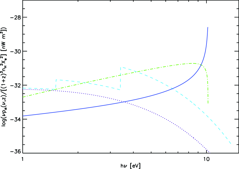
Figure 3: Volume emissivity spectrum of the IGM, $\nu p_{\alpha}(\nu,z)$, divided by $(1+z)^{3}n_{H}^{2}X_{e}^{2}$, for individual processes in units of nW m³ as a function of the rest-frame energies. (Note that this quantity does not depend on $z$.) We use the ionized gas temperature of $10^{4}$ K. Free-free (dotted purple line), free-bound (dashed light blue line), two-photon (dot dashed green line), and Lyman-$\alpha$ emission (solid dark blue line) are shown.

4 LUMINOSITY-DENSITY POWER SPECTRUM

The three-dimensional power spectrum of over-luminosity density, $\delta\rho_{L}({\mathbf{x}})$, is given by

$$\langle\widetilde{\delta\rho}_{L}({\mathbf{k}})\widetilde{\delta\rho}^{*}_{L}({\mathbf{k}}^{\prime})\rangle=(2\pi)^{3}P_{L}(k)\delta^{3}({\mathbf{k}}-{\mathbf{k}}^{\prime}),$$ (24)

where $P_{L}(k)$ is the luminosity-density power spectrum, and $\widetilde{\delta\rho}_{L}({\mathbf{k}})$ is the Fourier transform of the over-luminosity density field, $\delta\rho_{L}({\mathbf{x}})$. The over-luminosity density field is related to the excess in the volume emissivity over the mean, $\delta p(\nu,{\mathbf{x}})$, integrated over the observed bandpass $\nu_{1}$ to $\nu_{2}$, as

$$\delta\rho_{L}({\mathbf{x}},z)=\int_{\nu_{1}(1+z)}^{\nu_{2}(1+z)}d\nu~{}\delta p(\nu,{\mathbf{x}},z).$$ (25)

In the following derivations we do not write $z$ explicitly for clarity.

4.1 Halo Contribution

How do we calculate the halo contribution from a given simulation box at a given $z$? For the halo contribution, $\delta\rho_{L}^{\rm halo}$, we have

$$\delta\rho^{\rm halo}_{L}({\mathbf{x}})\equiv\left(\frac{L_{h}}{M_{h}}\right)\frac{M_{\rm cell}({\mathbf{x}})-\overline{M}_{\rm cell}}{V_{\rm cell}},$$ (26)

where $M_{\rm cell}({\mathbf{x}})$ is the total mass of halos within a given cell, $V_{\rm cell}$ is the volume of each cell, and the bars denote the volume average over the simulation box. Throughout this paper, we always include both the stellar contribution as well as the nebular contribution when we refer to the “halo contribution.”

Since we assume that halos have a constant mass-to-light ratio, $L_{h}/M_{h}$ does not depend on ${\mathbf{x}}$ or $M_{h}$ (but it depends on $z$), and is given by Eq. (9). Since we assume a constant mass-to-light ratio, the luminosity density $\delta\rho_{L}^{\rm halo}$ is linearly proportional to the halo mass density, $\delta\rho_{M}^{\rm halo}$, such that $\delta\rho_{L}^{\rm halo}({\mathbf{x}})=(L_{h}/M_{h})\delta\rho_{M}^{\rm halo}({\mathbf{x}})$, where $\delta\rho^{\rm halo}_{M}({\mathbf{x}})$ is the mass over-density of halos given by

$$\delta\rho^{\rm halo}_{M}({\mathbf{x}})\equiv\frac{M_{\rm cell}({\mathbf{x}})-\overline{M}_{\rm cell}}{V_{\rm cell}}=\int dM_{h}~{}M_{h}\left[\frac{dn_{h}({\mathbf{x}})}{dM_{h}}-\frac{d\bar{n}_{h}}{dM_{h}}\right].$$ (27)

Here, $dn_{h}({\mathbf{x}})/dM_{h}$ is the number density of halos per mass within a cell at a location ${\mathbf{x}}$, and $d\bar{n}_{h}/dM_{h}$ is its average. Therefore, the luminosity-density power spectrum of halos, $P^{\rm halo}_{L}(k)$, is simply proportional to the mass-density power spectrum of halos, $P^{\rm halo}_{M}(k)$, as

$$P^{\rm halo}_{L}(k)=\left(\frac{L_{h}}{M_{h}}\right)^{2}P^{\rm halo}_{M}(k).$$ (28)

The shape of $P^{\rm halo}_{L}(k)$ is determined by that of the halo mass-density power spectrum. In other words, one only needs to compute $P^{\rm halo}_{M}(k)$ from simulations, and the analytical calculations given in § 3.1 supply $L_{h}/M_{h}$ for a given stellar population and observed bandpass.

Specifically, we compute $P^{\rm halo}_{M}(k)$ from the simulation as follows (e.g., Jeong & Komatsu, 2009):

• Use the Cloud-In-Cell (CIC) mass distribution scheme to calculate the mass density field of halos on $256^{3}$ regular grid points, i.e., $M_{\rm cell}({\mathbf{x}})/V_{\rm cell}$, from the halo catalog.

• Fourier-transform the excess mass density, $[M_{\rm cell}({\mathbf{x}})-\overline{M}]/V_{\rm cell}$, using FFTW.

• Deconvolve the effect of the CIC pixelization effect. We divide $P(\mathbf{k},z)\equiv|\delta(\mathbf{k},z)|^{2}$ at each cell by the Fourier transform of the CIC kernel squared:

  $$W(\mathbf{k})=\prod_{i=1}^{3}\left[\frac{\sin\left(\frac{\pi k_{i}}{2k_{N}}\right)}{\frac{\pi k_{i}}{2k_{N}}}\right]^{4},$$ (29)

  where $\mathbf{k}=(k_{1},k_{2},k_{3})$, and $k_{N}\equiv\pi/H$ is the Nyquist frequency ($H$ is the physical size of the grid). In terms of the number of grids along one axis, $N_{\rm mesh}$, one may write $H=L_{\rm box}/N_{\rm mesh}$, and $2k_{N}=N_{\rm mesh}(2\pi/L_{\rm box})=N_{\rm mesh}\Delta k$, where $\Delta k=2\pi/L_{\rm box}$ is the fundamental frequency of the box. (For our simulation, $L_{\rm box}=100~{}h^{-1}~{}{\rm Mpc}$.) We also try a different deconvolution scheme that attempts to reduce the aliasing effect (Jing, 2005):

  $$W(\mathbf{k})=\prod_{i=1}^{3}\left[1-\frac{2}{3}\sin^{2}\left(\frac{\pi k_{i}}{2k_{N}}\right)\right].$$ (30)

  We then use $P_{M}(k)$ up to $k_{\rm max}$ below which both of the deconvolution schemes yield the same answer. We find $k_{\rm max}\sim 5~{}{\rm Mpc}^{-1}$.

• Compute $P_{M}(k,z)$ by taking the angular average of CIC-corrected $P(\mathbf{k},z)$ within a spherical shell defined by $k-\Delta k/2<|\mathbf{k}|<k+\Delta k/2$.

In the previous work on NIRB fluctuations (Kashlinsky et al., 2004; Cooray et al., 2004) the linear bias model was used, i.e., $P^{\rm halo}_{M}(k)$ was assumed to be linearly proportional to the underlying (linear) matter power spectrum. However, for such high redshifts halos are expected to be highly biased, and thus non-linear bias cannot be ignored. In other words, it is no longer correct to assume that $P^{\rm halo}_{M}(k)$ is linearly proportional to the underlying matter power spectrum.

To study this further, in Figure 4 we show $P_{M}^{\rm halo}(k)$ (in units of $M_{\sun}^{2}~{}{\rm Mpc}^{-3}$). Also shown in Figure 4 is the shot noise, $P_{M}^{shot}$, where $P_{M}^{shot}\equiv\int dM_{h}M_{h}^{2}d\bar{n}_{h}/dM_{h}$ ($d\bar{n}_{h}/dM_{h}$ is the mean halo mass function), the linear matter density fluctuations times the mean mass density squared ($P_{\rm lin}(k)(\bar{\rho}_{M}^{\rm halo})^{2}$), where $\bar{\rho}_{M}^{\rm halo}$ is the mean mass density of halos within the simulation box, and the bias, given by:

$$b_{\rm eff}(k)=\sqrt{\frac{P_{M}^{\rm halo}(k)-P_{M}^{shot}(k)}{(\bar{\rho}_{M}^{\rm halo})^{2}P_{\rm lin}(k)}}.$$ (31)

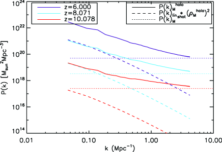
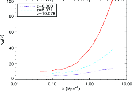
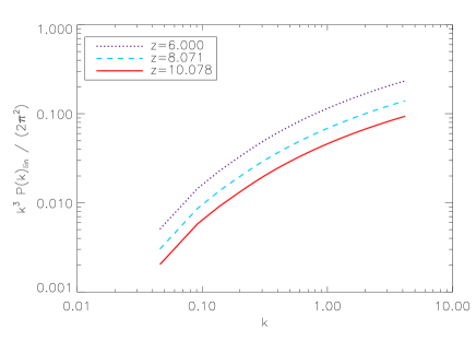
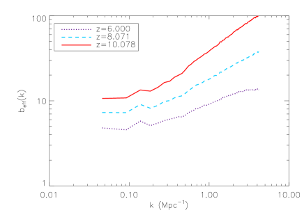
Figure 4: Non-linear bias of the halo mass-density power spectrum. (This is not the luminosity-density power spectrum; see § 4.1 for the precise definition.) Top left panel: The power spectra of the halo mass density, $P_{M}^{\rm halo}(k)$ are shown as the solid lines ($z=6$ to $10$ from top to bottom), the linear matter power spectra times the mean halo mass density squared, $P_{\rm lin}(k)(\bar{\rho}_{M}^{\rm halo})^{2}$, are the dashed lines, and the shot noise power spectra, $P_{M}^{shot}$, are the dotted lines. Top right panel: We show the bias, $\sqrt{[P_{M}^{\rm halo}(k)-P_{M}^{shot}(k)]/[(\bar{\rho}_{M}^{\rm halo})^{2}P_{\rm lin}(k)]}$, ($z=10$ to $6$ from top to bottom). The bias increases significantly as we go to smaller scales, and this effect has been ignored in the previous calculations of the power spectrum of NIRB fluctuations. Note that the minimum halo mass resolved in the simulation is $2.2\times 10^{9}~{}M_{\sun}$. The degree of non-linear bias would be smaller for a smaller minimum mass (see, e.g., Figure 6 of Trac & Cen, 2007). Bottom left panel: The linear power spectrum, $k^{3}P_{lin}(k)/(2\pi^{2})$. Bottom right panel: Same as top right panel, but on a log-log axis.

Figure 5: $\delta_{c}/\sigma(M_{Min},z)$ versus redshift. The halos resolved in our simulation, with $M>M_{\rm min}=2.2\times 10^{9}~{}M_{\sun}$, are located on rare peaks ($\delta_{c}/\sigma(M_{\rm min},z)\gtrsim 2.5$) at $z\gtrsim 7$.

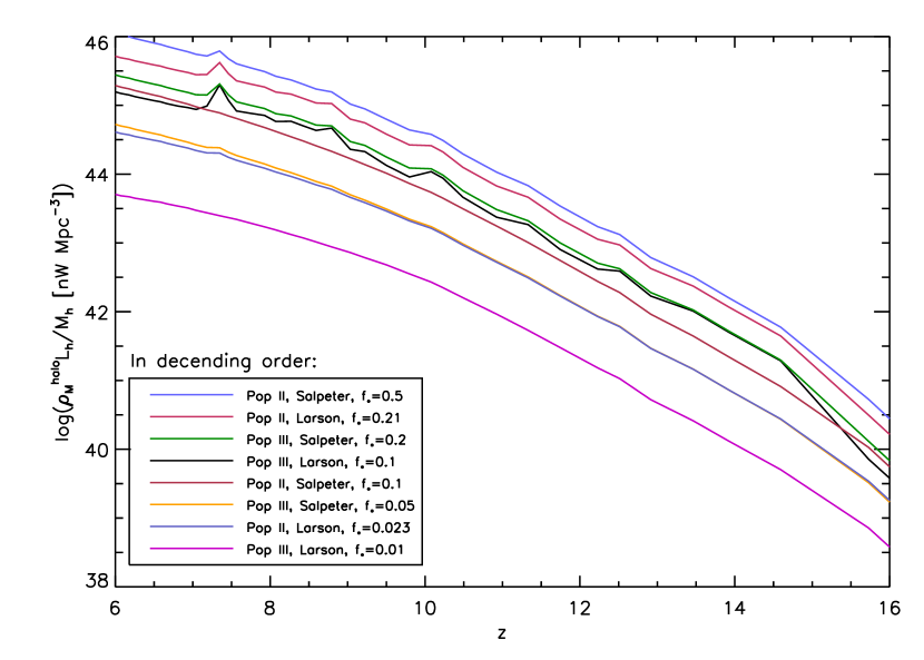
Figure 6: (Left) Mean halo luminosity density computed from our simulation, $\bar{\rho}_{M}^{\rm halo}(z)L_{h}(z)/M_{h}$, where $l^{\alpha}_{\nu}(z)$ is from equation (6), in units of nW Mpc^-3 as a function of redshifts, for various stellar populations given in Table 1. The waves in the lines where $f_{\rm esc}$ are higher are from the discrete redshift sampling of the Lyman-$\alpha$ line. We averaged the luminosity over a rectangular bandpass of $1-2~{}\mu{\rm m}$. (Right) Halo mass collapse fraction, $\bar{\rho}_{M}^{\rm halo}(z)/(\Omega_{m}\rho_{\rm c0})$, as a function of redshifts. The redshift evolution of $\bar{\rho}_{M}^{\rm halo}L_{h}/M_{h}$ is essentially determined by that of $\bar{\rho}_{M}^{\rm halo}$.

By comparing $P_{M}^{\rm halo}(k)$ (with the shot noise subtracted) with the power spectrum of linear matter density fluctuations times $(\bar{\rho}_{M}^{\rm halo})^{2}$, we find that, on large scales ($k\lesssim 0.1~{}{\rm Mpc}^{-1}$), they are related by $P_{M}^{\rm halo}(k)/(\bar{\rho}_{M}^{\rm halo})^{2}\approx b_{1}^{2}P_{\rm lin}(k)$ with the linear bias factor being $b_{1}\simeq 5$ at $z=6$ to $b_{1}\simeq 10$ at $z=10$, a highly biased population. The bias increases monotonically as we go to smaller scales, significantly boosting the power in the halo distribution relative to the matter distribution. This changes the prediction for the shape of the angular power spectrum qualitatively, compared with the previous results given in the literature (Cooray et al., 2004; Kashlinsky et al., 2004). This behavior of non-linear bias with redshift is consistent with that expected from the halo model (Cooray & Sheth, 2002). These halos are very rare, located on high peaks with $\delta_{c}/\sigma(M_{min},z)\gtrsim 2.5$ (see Figure 5).

This motivates our writing $P^{\rm halo}_{L}(k)$ as

$$P^{\rm halo}_{L}(k)=\left(\frac{\bar{\rho}_{M}^{\rm halo}L_{h}}{M_{h}}\right)^{2}b_{\rm eff}^{2}(k)P_{\rm lin}(k),$$ (32)

where the pre-factor, $\bar{\rho}_{M}^{\rm halo}L_{h}/M_{h}$, is the mean halo luminosity density. In the left panel of Figure 6 we show $\bar{\rho}_{M}^{\rm halo}L_{h}/M_{h}$ (in units of nW Mpc^-3) as a function of redshifts. We find that the redshift evolution of $\bar{\rho}_{M}^{\rm halo}L_{h}/M_{h}$ is very rapid; thus, the redshift evolution of the halo luminosity density power spectrum, $P^{\rm halo}_{L}(k)$, is dominated by that of the mean halo luminosity density.

What determines the evolution of the mean halo luminosity density? The answer is simple: it is determined by the rate at which the mass in the universe collapses into halos. To show this, in the right panel of Figure 6 we show the halo mass collapse fraction, or the ratio of $\bar{\rho}_{M}^{\rm halo}$ to the mean comoving mass density of the universe, $\Omega_{m}\rho_{\rm c0}$, where $\rho_{\rm c0}=2.775\times 10^{11}~{}h^{2}~{}M_{\sun}~{}{\rm Mpc}^{-3}$ is the critical density of the universe at the present epoch. The evolution of the collapse fraction is fast, explaining the fast evolution of the mean halo luminosity density.

As halos are discrete objects, and we do not expect to resolve individual halos contributing to the diffuse NIRB, the observed NIRB power spectrum is a sum of the clustering component and the shot noise component. If the shot noise dominates over the clustering component, it would be very difficult to ascertain information on the structure from the signal of the NIRB. The shot noise component can be estimated by integrating the luminosity squared over the mass function:

$$P_{L}^{shot}=\left(\frac{L_{h}}{M_{h}}\right)^{2}P_{M}^{shot}=\left(\frac{L_{h}}{M_{h}}\right)^{2}\int dM_{h}~{}M_{h}^{2}\frac{d\bar{n}_{h}}{dM_{h}},$$ (33)

where we have again assumed that each halo has a constant mass-to-light ratio, i.e., $L_{h}/M_{h}$ is independent of $M_{h}$.

4.2 IGM Contribution

For the IGM contribution, we have

$$\delta\rho^{\rm IGM}_{L}({\mathbf{x}})=\left(\frac{{p^{\rm IGM}}}{n_{H}^{2}X_{e}^{2}}\right)\left[C_{\rm cell}({\mathbf{x}})n_{\rm cell}^{2}({\mathbf{x}})X^{2}_{e,\rm cell}({\mathbf{x}})-\overline{(C_{\rm cell}n_{\rm cell}^{2}X_{e,\rm cell}^{2})}\right],$$ (34)

where $p^{\rm IGM}$ is the volume emissivity of the IGM, integrated over the observed frequencies, i.e., $p^{\rm IGM}\equiv\int_{\nu_{1}(1+z)}^{\nu_{2}(1+z)}d\nu p^{\rm IGM}(\nu)$, $C_{\rm cell}$, $n_{\rm cell}$, $X_{e,\rm cell}$ are the clumping factor, the comoving number density of hydrogen atoms, and the ionization fraction within a cell, respectively. We compute $n_{\rm cell}$ using

$$n_{\rm cell}=\frac{\Omega_{b}}{\Omega_{m}}\frac{\rho_{M,\rm cell}}{\mu m_{p}},$$ (35)

where $\mu=0.59$ and $m_{p}$ are the mean molecular weight of ionized gas and the proton mass, respectively. We have used the mass density of $N$-body particles per cell, $\rho_{M,\rm cell}$, multiplied by the baryon fraction, $\Omega_{b}/\Omega_{m}$, for computing the mass density of baryons per cell, as we have assumed that gas traces dark matter particles, i.e., $N$-body particles. The clumping factor, $C_{\rm cell}\equiv n^{2}_{actual}/n_{\rm cell}^{2}$, relates the actual density squared to the square of the density averaged within a cell. In other words, $C_{\rm cell}$ captures the sub-grid clumping that is not resolved by the simulation.

Following Iliev et al. (2007), we make a simplifying assumption that $C_{\rm cell}$ takes on the same value everywhere in the simulation, and evolves with redshift $z$ as $C_{\rm cell}(z)=26.2917e^{-0.1822z+0.003505z^{2}}$; thus, we have

$$\delta\rho^{\rm IGM}_{L}({\mathbf{x}})=26.2917e^{-0.1822z+0.003505z^{2}}\left(\frac{p^{\rm IGM}}{n_{H}^{2}X_{e}^{2}}\right)\left[n_{\rm cell}^{2}({\mathbf{x}})X^{2}_{e,\rm cell}({\mathbf{x}})-\overline{(n_{\rm cell}^{2}X_{e,\rm cell}^{2})}\right].$$ (36)

Note that $p^{\rm IGM}/(n_{H}^{2}X_{e}^{2})$ does not depend on ${\mathbf{x}}$, and is given by Eq. (23) integrated over a rectangular bandpass of $1-2~{}\mu$m in the observer’s frame.

5 RESULTS

5.1 Luminosity-density Power Spectrum

In Figures 7 and 8 we show the luminosity-density power spectra, $P_{L}(k)$, for halos and their associated HII regions in the IGM for two of our populations: Population II stars with a Salpeter initial mass spectrum with $f_{\rm esc}=0.19$ and $f_{*}=0.5$ (Figure 7) and Population III stars with a Larson initial mass spectrum with $f_{\rm esc}=1$ and $f_{*}=0.01$ (Figure 8), assuming a rectangular bandpass from $1-2$ $\mu{\rm m}$.

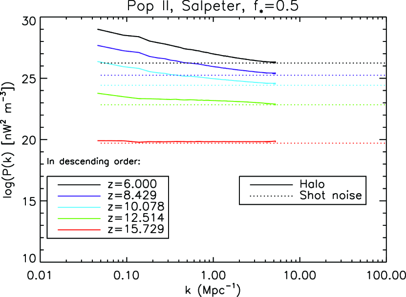
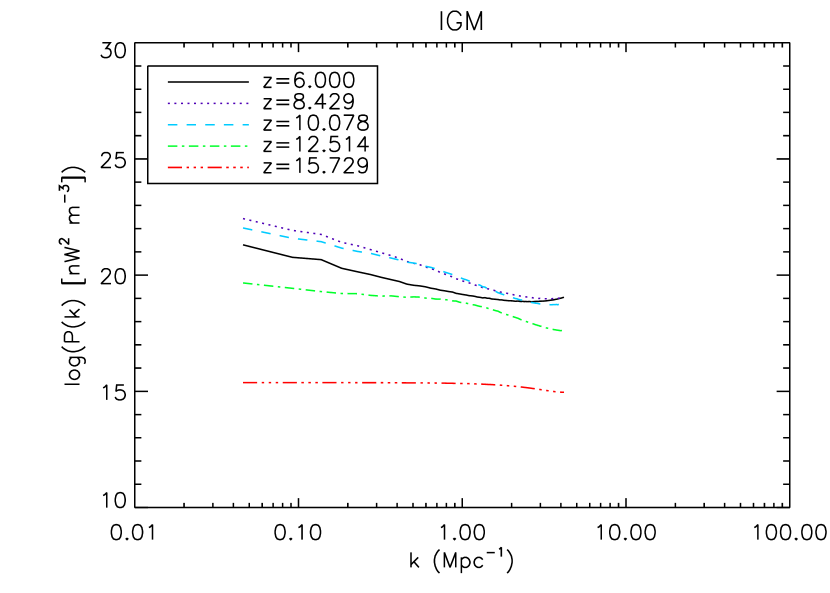
Figure 7: (Left) Luminosity-density power spectrum of halos with Pop II stars obeying a Salpeter initial mass spectrum, $f_{\rm esc}=0.19$, and $f_{*}=0.5$, assuming a rectangular bandpass from $1-2$ $\mu{\rm m}$. The shot noise for the halo contribution is also shown as the dotted lines. (Right) Luminosity-density power spectrum of the IGM. The ionization fraction of the IGM reaches 0.5 at about $z\sim 8.3$. On large scales where the shot noise is sub-dominant, we find $P_{L}(k)\propto k^{-3/2}$, which yields $C_{l}\propto l^{-3/2}$ or $l^{2}C_{l}\propto l^{1/2}$ (see § 5.2).

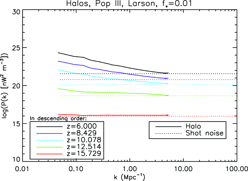
Figure 8: (Left) The same as the left panel of Figure 7 with Pop III stars with the Larson initial mass spectrum, $f_{\rm esc}=1$, and $f_{*}=0.01$. (Right) The same as the right panel of Figure 7 for comparison.

The luminosity-density power spectra of halos are approximately power-laws over the entire range of wavenumbers that the simulation covers. At the highest redshift bin, $z\sim 16$, the power spectrum is entirely dominated by the shot noise at all scales. The lower the redshifts are, the more power in excess of the shot noise we observe on large scales (because the shot noise is most important on small scales). The growth of the power spectrum is partly driven by the growth of linear matter fluctuations as well as that of halo bias, i.e., the clustering of halos is biased relative to the underlying matter distribution. As we have shown in the previous section, the bias of halos that we observe in the simulation is highly non-linear, and thus has an important implication for the predicted shape of the observed power spectrum of NIRB fluctuations. However, as we have shown in § 4.1, the evolution of $P_{L}(k)$ is almost entirely driven by the fast growth of the mean halo luminosity density, $\bar{\rho}_{M}^{\rm halo}(z)L_{h}(z)/M_{h}$ (see Eq. (32) and the left panel of Figure 6). As a result $P_{L}(k)$ grows by about six orders of magnitude at $k=0.1~{}{\rm Mpc}^{-1}$ from $z\sim 13$ to $z\sim 6$, which is much faster than the growth expected from the growth of bias times the matter power spectrum.

The luminosity-density power spectrum of the IGM increases quickly as the mean ionization fraction, $\bar{X}_{e}$, approaches 0.5 (at about $z\sim 8.3$ for this particular simulation), especially on larger scales. As the ionization fraction increases, the luminosity of the HII region would also increase (because luminosity is proportional to $X_{e}^{2}$). Moreover, since we are looking at the over-luminosity-density power spectrum of the IGM, the greatest power results when there is the greatest difference between luminous regions and the average luminosity of the IGM; thus, the power spectrum of $X^{2}_{e}n^{2}$ grows rapidly as $\bar{X}_{e}$ approaches 1/2. However, this rapid growth of the power stops when the entire IGM is ionized ($\bar{X}_{e}=1$), in which case the over-luminosity-density power spectrum of the IGM is simply proportional to $n^{2}$.

The most interesting feature of the luminosity-density power spectrum of the IGM is a “knee” feature, which is at $k\sim 2~{}{\rm Mpc}^{-1}$ at $z\sim 16$, and moves to $k\lesssim 1~{}{\rm Mpc}^{-1}$ at $z\lesssim 10$. This “knee” is caused by the typical size of HII bubbles: the knee wavenumber is inversely proportional to the typical size of the bubbles. At the highest redshift bin, $z\sim 16$, the bubbles are nearly Poisson-distributed, and thus the power spectrum is flat up to the knee scale, $k\sim 2~{}{\rm Mpc}^{-1}$, beyond which the power decreases as one is looking at the scales inside the bubbles, which are smooth. As the redshift decreases, the knee scale moves to larger scales, signifying a growth in the ionized bubbles with time until they merge. At the same time, the large-scale power also grows, and the shape of the HII region power spectrum is basically the same as that of the halo power spectrum, as the bubbles are created around the halos.

Note that Iliev et al. (2006, 2007) studied the power spectrum of ionized gas density, and observed a similar trend. The power spectrum of the luminosity density that we have presented here is the four-point function of the ionized gas density (as the volume emissivity is proportional to the ionized gas density squared), and thus it is different from the power spectrum of the ionized gas density (which is quadratic in density).

5.2 Angular Power Spectrum of NIRB Fluctuations

What about the observable, the angular power spectrum of NIRB fluctuations, $C_{l}$? We compute the angular power spectrum of NIRB fluctuations, $C_{l}$, by projecting $P_{L}(k)$ on the sky. We do this using Limber’s approximation, and obtain (see Appendix A for the derivation)

$$C_{l}=\frac{c}{(4\pi)^{2}}\int\frac{dz}{H(z)r^{2}(z)(1+z)^{4}}P_{L}\left(k=\frac{l}{r(z)},z\right),$$ (37)

where $r(z)=c\int^{z}_{0}dz^{\prime}/H(z^{\prime})$ is the comoving distance. We integrate Eq. (37) over the range of redshifts that the simulation covers for both halos and the IGM, $z=6.0-15.7$.

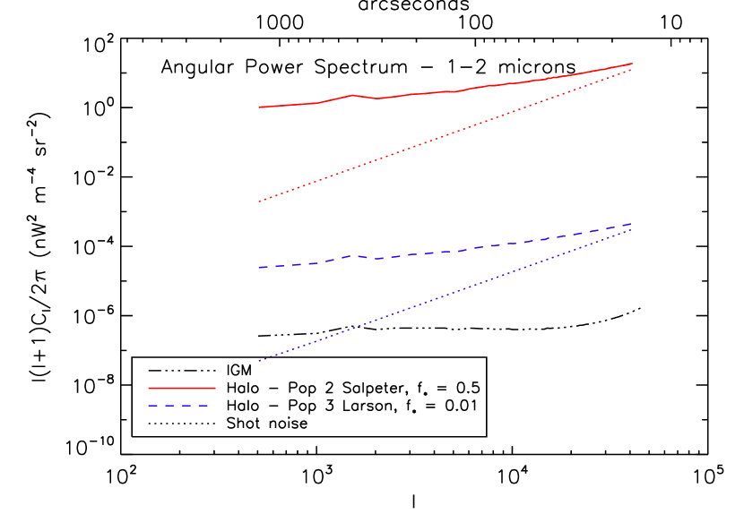
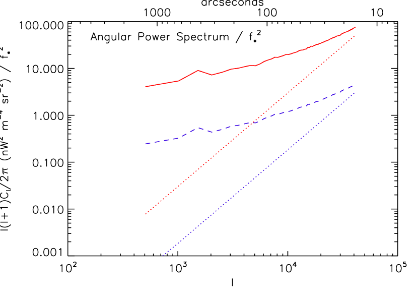
Figure 9: Angular power spectra of NIRB fluctuations, $C_{l}$, from halos in comparison to the angular power spectrum of the IGM (the bottom line). We show $C_{l}$ from halos that have Population II stars with a Salpeter mass spectrum and $f_{*}=0.5$ (the angular power spectrum that has the highest amplitude) and Population III stars with a Larson mass function and $f_{*}=0.01$ (the angular power spectrum with the lowest amplitude and which is closest to the angular power spectrum of the IGM). The dotted lines show the level of the shot noise. In Figure 11 we show how the amplitude of the power spectrum changes between populations with various escape fractions of the ionizing photons into the IGM, $f_{\rm esc}$, and star formation efficiencies, $f_{*}$. (Right panel) Same as the left panel, except divided by $f_{*}^{2}$. The IGM contribution is not shown.

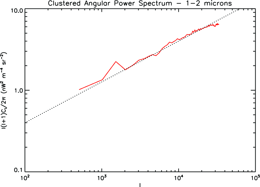
Figure 10: The angular power spectrum from the clustering of halos (solid line), i.e., the angular power spectrum minus the shot noise contribution. The dotted line has a slope of $l^{0.5}$. The clustered angular power spectrum shows no evidence of a turnover that was claimed to exist in the literature. This is because previous analytical models in the literature based their power spectrum on the linear bias model, which is not valid for this population, which has a high level of non-linear bias. The minimum halo mass used in this calculation is $2.2\times 10^{9}~{}M_{\sun}$.

In Figure 9 we show $l(l+1)C_{l}/(2\pi)$ for halos with Population II stars with a Salpeter mass spectrum and $f_{*}=0.5$ (the angular power spectrum for halos with the highest amplitude) and for Population III stars with a Larson mass spectrum and $f_{*}=0.01$ (the angular power spectrum for halos with the lowest amplitude), along with the angular power spectrum of the IGM. The halo contribution at small scales, i.e., $l\gtrsim 10^{4}$, is comparable to the shot noise contribution. When the shot noise is subtracted (see Figure 10), we find that $l(l+1)C_{l}/(2\pi)$ is nearly a power-law, $l(l+1)C_{l}/(2\pi)\propto l^{0.5}$, with no sign of a turn-over, which would be expected from the shape of the projected linear matter power spectrum. This is in a stark contrast with the previous calculations (Kashlinsky et al., 2004; Cooray et al., 2004), which predicted a turn-over at $l\sim 10^{3}$. They assumed that the luminosity-density power spectrum was given by the linear bias model, in which the halo power spectrum is a constant times the matter power spectrum. Our calculations, which are based on a realistic simulation, indicate that the simple linear bias model is not valid for these populations. This is expected, as these populations are very highly biased, and therefore non-linear bias must also be large, as demonstrated already in Figure 4.

On the other hand, there is no freedom in changing the amplitude of the IGM power spectrum for a given simulation, i.e., a given $f_{\gamma}/t_{\rm SF}$; thus, we show only one line for the IGM contribution in Figure 9 (the lowest line). For the parameter space explored here, the halo contribution can be as low as being only slightly over an order of magnitude (for PopIII Larson with $f_{\rm esc}=1$ and $f_{*}=0.01$) to about $10^{6}$ times greater (for PopII Salpeter with $f_{\rm esc}=0.19$ and $f_{*}=0.5$) than the IGM contribution. If we were to increase $f_{\gamma}$ (which is possible using additional simulations in future work, although one has to make sure that the resulting electron-scattering optical depth is consistent with the WMAP data), a wider range of parameters $f_{\rm esc}$, $f_{*}$ and $N_{i}$ could result. This is a good news, as this gives us an opportunity to study the physics of the reionization using the power spectrum of NIRB fluctuations. Sensitive surveys may be able to detect a change in the shape of the power spectra that would be a result of the IGM power spectrum. This may be one way of constraining $f_{\rm esc}$ observationally.

In Figure 11, we show the amplitude of the angular power spectra of other stellar populations scaled to the angular power spectrum of Population II stars with a Salpeter mass spectrum and $f_{*}=0.5$. As we find in Eq. (9), the luminosity-density power spectrum of halos is about proportional to $f_{*}^{2}$, and one of the terms in the power spectrum (nebular contribution; the second term in Eq. (9)) depends on $(1-f_{\rm esc})$. Therefore, for a fixed $f_{\gamma}=f_{\rm esc}f_{*}N_{i}$ and fixed $N_{i}$ (i.e., fixed stellar population), the angular power spectrum of the halo contribution must always increase as we increase $f_{*}$, as increasing $f_{*}$ must be accompanied by the corresponding reduction in $f_{\rm esc}$, both of which will increase the power spectrum of the halo contribution.

Figure 11: (Left panel) The change of the angular power spectrum as a function of the escape fraction, $f_{\rm esc}$, for our selected samples of stellar populations. Each amplitude is scaled with relation to the angular power spectrum of Population II stars with a Salpeter mass spectrum and $f_{*}=0.5$. (Since the shape of the angular power spectra are the same for all stellar populations, this ratio is the same for all wave numbers.) (Right panel) The dependence of the angular power spectrum on $f_{*}$. The solid line shows $C_{l}\propto f_{*}^{2}$. Note that each stellar population has a different set of $f_{*}$, $f_{\rm esc}$, and $N_{i}$, and thus both panels show a slice of the multi-parameter space.

As $C_{l}\propto f_{*}^{2}$, the parameter combinations that maximize $f_{*}$ tend to give the largest $C_{l}$. For a fixed $f_{\gamma}=f_{\rm esc}f_{*}N_{i}$ this means a lower $N_{i}$, i.e., lighter mass spectra with larger metallicity (see the 5th column of Table 1), and a lower $f_{\rm esc}$. In reality, however, we should also take into account the fact that heavier mass spectra produce more luminosity per stellar mass, i.e., more $\bar{l}$ in Eq. (9). These factors explain the dependence of the predicted amplitudes of $l(l+1)C_{l}/(2\pi)$ (averaged over $\lambda=1-2~{}\mu{\rm m}$) on parameters shown in Figure 11. Populations with higher $f_{\rm esc}$ have lower angular power spectrum. This is to be expected, because as $f_{\rm esc}$ increases, less photons are available to create luminosity within the halo.

6 VARYING THE MODEL: HALO CONTRIBUTION

In this section, we will focus on the halo contribution to the angular power spectrum of NIRB fluctuations, and explore the effects of changing various parameters.

6.1 THE EFFECT OF THE STAR FORMATION TIMESCALE

As mentioned in section 3.1, the star formation timescale will affect the amplitude of the angular power spectrum. We have assumed in this work a constant star formation timescale of $t_{\rm SF}=20$ Myr to make a consistent comparison between the halo and the IGM contributions. However, the amplitude of $C_{l}$ from halos depends sensitively on this rather uncertain timescale, as the luminosity of halos is proportional to $t_{\rm SF}^{-1}$, and thus $C_{l}\propto 1/t_{\rm SF}^{2}$. Motivated by this, in this section we consider two other possibilities: 1) The star formation time scale is shorter than the lifetime of the stars, in which case we will use equation 7 to compute the luminosity per mass, and 2) the star formation is triggered by mergers, i.e.,

$$t^{-1}_{\rm SF}(z)=\frac{\int dM_{h}M_{h}(d^{2}n_{h}/dM_{h}dt)}{\int dM_{h}M_{h}(dn_{h}/dM_{h})},$$ (38)

where $dn_{h}/dM_{h}$ is the mass function of dark matter halos. For the Press-Schechter mass function, we can calculate $t_{\rm SF}(z)$ analytically from

$$t_{\rm SF}^{-1}=H(z)\left|\frac{d\ln D}{d\ln(1+z)}\right|\left[\frac{\delta_{c}^{2}}{D^{2}(z)\sigma^{2}(M_{\rm min})}-1\right]\approx H(z)\Omega_{m}^{0.55}(z)\left[\frac{\delta_{c}^{2}}{D^{2}(z)\sigma^{2}(M_{\rm min})}-1\right],$$ (39)

where $\delta_{c}=1.68$, $D(z)$ is the growth factor of linear matter density fluctuations normalized such that $D(0)=1$, $\sigma(M_{\rm min})$ is the present-day r.m.s. matter density fluctuation smoothed over a top-hat filter that corresponds to the minimum mass $M_{\rm min}$, and $\Omega_{m}(z)$ is the matter density parameter at a given $z$. Note that interpreting this quantity as a merger timescale makes sense only when we study the density peaks above the r.m.s., i.e., $\delta_{c}/[D(z)\sigma(M_{\rm min})]>1$. (Otherwise $t_{\rm SF}$ becomes negative.) This formula has a clear physical interpretation: for a density peak of order the r.m.s. mass density fluctuation, $\delta_{c}/[D(z)\sigma(M_{\rm min})]-1\approx 1$, the merger timescale is of order the Hubble time, i.e., $t_{\rm SF}\approx H^{-1}(z)$. The higher the peaks are, the shorter the merger timescale becomes; thus, in this model, high-$z$ objects (for a given mass) have shorter star formation timescales, and are brighter.

As the reionization history depends on $f_{\gamma}/t_{\rm SF}$, changing only $t_{\rm SF}$ without the corresponding change in $f_{\gamma}$ results in a different reionization history. For example, increasing $t_{\rm SF}$ by a factor of 10 makes individual sources fainter by a factor of 10, and thus it would result in a much slower reionization history. To compensate this one would have to increase $f_{\gamma}$ by a factor of 10. Moreover, if we reduce $t_{\rm SF}$ by a large factor, it would make individual sources brighter by a large factor, to the point where we might start detecting these sources individually, e.g., as Lyman-$\alpha$ emitters (Fernandez & Komatsu, 2008).

In this section, however, we explore the effects of $t_{\rm SF}$ for a given $f_{\gamma}$, to show how important this quantity is for predicting the amplitude of NIRB fluctuations without any extra information on reionization from WMAP or Lyman-$\alpha$ emitters.

The angular power spectrum for various assumptions for the star formation timescale is given in Figure 12. The angular power spectrum with the highest amplitude corresponds to when the star formation time scale is shorter than the lifetime of the stars. If the star formation timescale is given by the merger time of halos (Eq. 39), the star formation timescale varies with redshift and we obtain the lowest amplitude for the angular power spectrum, as the merger timescale at a given redshift is usually comparable to the age of the Universe at the same redshift. Our assumption of $t_{\rm SF}=20$ Myr lies between these two extremes.

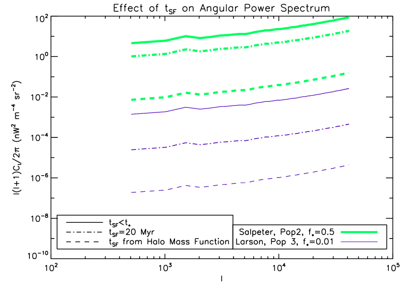
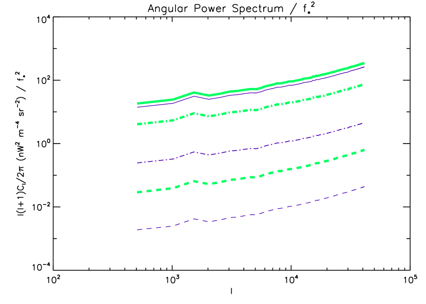
Figure 12: The effect of the star formation time scale on the angular power spectrum. We find the largest amplitudes when $t_{\rm SF}$ is shorter than the main sequence lifetime of stars, whereas we find the lowest amplitudes when $t_{\rm SF}$ is given by the timescale of halo mergers (Eq. 39). The uncertainty due to the star formation time scale is large and can lead to an uncertainty in the angular power spectrum of a factor of $\approx 10^{4}$. This reflects our uncertainty in the mass to light ratio of galaxies that contribute to the NIRB. However, note that not all scenarios shown here yield the reionization histories that are consistent with the WMAP data and the abundance of Lyman-$\alpha$ emitters. (Right panel) Same as the left panel, except divided by $f_{*}^{2}$.

We can further quantify the uncertainty in $C_{l}$ from $t_{\rm SF}$ by looking at the mass-to-light ratio of the galaxies (see Figure 13). We know very little about the nature of high-$z$ galaxies contributing to NIRB. We don’t know what the mass-to-light ratio is for these populations. An uncertainty of a factor of 100 in the star formation timescale will correspond directly to an uncertainty in the mass-to-light ratio of 100, and an uncertainty of $10^{4}$ in the angular power spectrum. Early galaxies could be starbursts, with a mass-to-light ratio of less than 0.1 to 1, or normal galaxies, with a mass-to-light ratio of $\gtrsim 10$. The amplitude of $C_{l}$ is, among other things, a sensitive probe of the nature of high-$z$ galaxies.

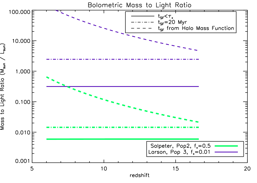
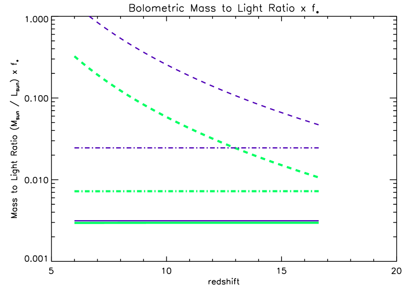
Figure 13: The bolometric mass-to-light ratio for halos for various star formation timescales. Uncertainty in the amplitude of the star formation time scale can be equated to the uncertainty in the mass-to-light ratio, i.e., the nature of high-$z$ galaxies contributing to the NIRB. The upper and lower sets of lines show the PopIII Larson and the PopII Salpeter, respectively. (Right panel) Same as the left panel, except multiplied by $f_{*}$.

6.2 THE EFFECT OF CHANGING $z_{\rm end}$

The angular power spectra will also depend on what we choose for the end of the star formation epoch, $z_{\rm end}$. The effect of our choice of $z_{\rm begin}$ is minimal, because at high redshift, the halos are smaller and dimmer, contributing less to the angular power spectrum. (See Figures 7 and 8.) Since halos and IGM will contribute more to fluctuations at lower redshifts, we find that the angular power spectrum dramatically drop as we stop star formation at higher redshifts (see Figure 14).

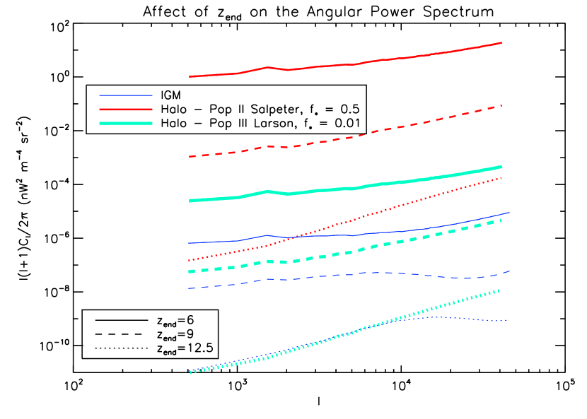
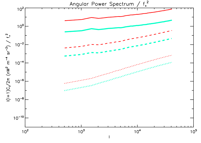
Figure 14: The angular power spectrum for halos and IGM as $z_{\rm end}$ is varied. We show the angular power spectrum for the halos with the highest and lowest amplitude of the angular power spectrum (Population II stars with a Salpeter mass spectrum and $f_{*}=0.5$ and Population III stars with a Larson mass spectrum and $f_{*}=0.01$ respectively) and the IGM. The angular power spectrum as shown throughout the rest of the paper has $z_{\rm end}=6$. As $z_{\rm end}$ increases, the angular power spectrum drops. At very high redshifts, the angular power spectrum of the IGM is higher than some of the angular power spectrum of the halos. (Right panel) Same as the left panel, except divided by $f_{*}^{2}$. The IGM contribution is not shown.

The shape of the angular power spectrum also changes as we vary $z_{\rm end}$. As $z_{\rm end}$ increases, the angular power spectrum of the halos steepens. The shape of the angular power spectrum from the IGM can also affect the overall slope of the observed angular power spectrum if the halo contribution is close to that of the IGM contribution. If the escape fraction is small, this effect in the change of shape from the IGM will be less than if the escape fraction is large. When $z_{\rm end}$ is very large, the amplitude of the angular power spectrum of the IGM could even be higher than that of the halos.

6.3 LYMAN-$\alpha$ ATTENUATION

The Lyman-$\alpha$ line can be attenuated by dust or neutral hydrogen. To understand this effect one would have to perform detailed calculations of the radiation transport of Lyman-$\alpha$ photons, including scattering of Lyman-$\alpha$ photons; however, such calculations are usually quite complex and time-consuming. Therefore, in this subsection we study the extreme limit of attenuation: the case where all of the Lyman-$\alpha$ photons are absorbed or extinct. How would this affect the angular power spectrum? The effect of the complete Lyman-$\alpha$ attenuation is shown in Table 2.

Population	Initial Mass Spectrum	$f_{\rm esc}$	$f_{*}$	$C_{l,\>Ly\alpha\>atten}/C_{l,\>no\>atten}$
Pop III	Salpeter	0.22	0.2	0.848
Pop III	Larson	0.1	0.1	0.632
Pop III	Salpeter	0.9	0.05	0.975
Pop III	Larson	1	0.01	1
Pop II	Salpeter	0.95	0.1	0.995
Pop II	Larson	0.9	0.023	0.974
Pop II	Salpeter	0.19	0.5	0.926
Pop II	Larson	0.098	0.21	0.825
IGM				0.448

Table 2: The effect of Lyman-$\alpha$ attenuation on the angular power spectrum. Here, we assume complete attenuation (no production of Lyman-$\alpha$ photons). The angular power spectrum is only slightly affected in most cases, and is more affected in cases where the Lyman-$\alpha$ line was strong to begin with (such as heavy Pop III stars). The effect of Lyman-$\alpha$ attenuation in the IGM is the highest, as the IGM does not have the stellar contribution, and is mainly dominated by the Lyman-$\alpha$ and two-photon emission.

The effect of the Lyman-$\alpha$ attenuation is the greatest when the Lyman-$\alpha$ line is the strongest (for heavy Pop III stars) and when the escape fraction is smaller (so more photons stay within the halo to produce nebular emission). The effect of Lyman-$\alpha$ attenuation in the IGM is the highest, because normally a higher fraction of emission is coming from the Lyman-$\alpha$ line (in the halos, there is also stellar emission).

7 COMPARISON TO PREVIOUS WORK

Cooray et al. (2004) made fully analytic predictions of the angular power spectrum in the NIRB luminosity expected from the first stars in halos. They ignored the IGM contribution, which we found to be small relative to the halo contribution for a range of parameters we have explored in this paper. They modeled halos with 300 solar mass stars for two cases: (1) an optimistic scenario - star formation in halos above $10^{5}$ K, halos forming stars from $z=10-30$, and a star formation efficiency of 100%; and (2) a pessimistic scenario - star formation beginning at 5000 K (so the bias is lower), halos forming stars from $z=15-30$, and a star formation efficiency of 10%. Using the same stellar masses ($300~{}M_{\sun}$), we have compared our results from the simulation to the optimistic case from Cooray et al. (2004) for two different escape fractions, 0 and 1, and show the results in Figure 15 for different wavelengths. As in Cooray et al. (2004), we use the star formation time scale given by the merger time scale (see Eq. 38). The angular power spectrum here is

$$C_{l}^{\nu\nu^{\prime}}=\frac{c}{(4\pi)^{2}}\int\frac{dz}{H(z)r^{2}(z)(1+z)^{2}}P_{p}\left(\nu(1+z),\nu^{\prime}(1+z);k=\frac{l}{r(z)},z\right),$$ (40)

which gives the angular power spectrum at only one wavelength (rather than that averaged over a certain bandpass). The difference between this equation and Eq. (37) is a factor of $(1+z)^{2}$ since we are no longer integrating over a range of frequencies (see Appendix A for the derivation). Note that we do not show $C_{l}$ at $1~{}\mu{\rm m}$: at $1~{}\mu{\rm m}$, the emission comes from photons that are more energetic than $h\nu=13.6$ eV in the rest frame at $z>10$. Because of this, there should be no emission from the halos themselves, if one considers halos at $z>10$. (There would be contributions if one considered halos at lower redshifts, say, $z>6$.)

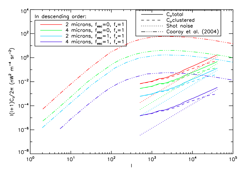
Figure 15: Comparison to Cooray et al. (2004) (shown as triple-dot dashed lines). We show $l(l+1)C_{l}/(2\pi)$ where $C_{l}=\nu^{2}C_{l}^{\nu\nu}$ (see Eq. 40), from halos at $z>10$ that host only very massive stars with $300~{}M_{\sun}$, at various wavelengths. The total angular power spectra from this work are shown as solid lines, shot noise is shown as dotted lines, and the clustered angular power spectra, which are the total power minus the shot noise components, are shown as dashed lines. Note that the amplitudes of $C_{l}$ shown here are much smaller than those shown in the previous figures (despite a high star formation efficiency, $f_{*}=1$), as we have removed the most dominant, lower redshift contributions, $z<10$, in this figure, to be compatible with Cooray et al. (2004). See Figure 14 for the effects of changing the minimum redshift of star formation. The mean intensity, $\nu I_{\nu}$, for this population of stars at $2\mu{\rm m}$ and $4\mu{\rm m}$ are $63$ and $16$  nW m^-2 sr^-1 respectively, which is already ruled out by observations (see section 9).

Since there were not enough halos in our simulation to create an accurate power spectrum above $z=16.6$, our population of stars only goes from $10<z<16.6$, while the model from Cooray et al. (2004) included star formation from $10<z<30$. However, this should not make too much of a difference, because halos at higher redshift do not contribute as much to the angular power spectrum. In Figure 15 we show the angular power spectrum minus the shot noise, which will give us the angular power spectrum of the clustered component, which is directly comparable to the quantity from Cooray et al. (2004). We have included all the nebular processes including the free-bound and two-photon emission, which are important to the overall luminosity of the halo and which Cooray et al. (2004) have neglected. The overall amplitude of our angular power spectrum is lower than that which Cooray et al. (2004) predicted, by a large factor, $10^{3}$.

In addition, the angular power spectrum from Cooray et al. (2004) peaks at about $l\sim 1000$ and then turns over. This is because Cooray et al. (2004) did not take into account the nonlinear bias in the halo power spectrum. Nonlinear bias will increase the power at small scales, especially at high redshifts, where galaxies were more highly biased. We again refer to Figure 4, which shows the importance of non-linear bias. This greatly affects both the amplitude and the shape of the angular power spectrum of the NIRB and should be included.

8 OBSERVING THE FLUCTUATIONS IN THE NEAR INFRARED BACKGROUND

Interpretation of the NIRB data can be a challenging task. Instrument emission, foregrounds and zodiacal light must all be taken into account. Foreground stars and low-redshift galaxies, in addition to very faint and the dim wings of galaxies, must be removed. Much of the differences in the existing measurements of the fluctuations from stars at high redshift result from differences in how lower redshift galaxies are accounted for. Foreground galaxies are removed down to a limiting magnitude (which is usually different between different observations). Galaxies fainter than this are taken into account using different methods.

There have been several observations of the NIRB. Kashlinsky & Odenwald (2000) found fluctuations at the wavelengths from ${\rm 1.25}$ to ${\rm 4.9}\>\mu{\rm m}$ in the images taken by the Diffuse Infrared Background Experiment (DIRBE) on Cosmic Background Explorer (COBE), which were not consistent with the Galactic emission or instrument noise. Matsumoto et al. (2005) observed the NIRB using the Infrared Telescope in Space (IRTS). They detected a clustering excess on scales of about $100^{\prime}$ from 1.4 to 4 $\mu{\rm m}$, and an indication of a spectral jump from the high redshift Lyman cutoff. This jump could indicate that Population III star formation ended at about a redshift of $z\sim 9$. Excess fluctuations were detected, possibly from high redshift galaxies, at about 1/4 of the mean intensity. Kashlinsky et al. (2007c, 2005) made observations of the fluctuations of the NIRB using the Infrared Array Camera (IRAC) on the Spitzer Space Telescope at 3.6, 4.5, 5.8 and 8 $\mu{\rm m}$. Sources were removed by clipping pixels containing $\gtrsim 4\sigma$ peaks, as well as removing fainter sources identified by SExtractor and convolved with the appropriate point spread function of IRAC. Since zodiacal light is not fixed in celestial coordinates, it was removed by taking observations six months apart in fields rotated by 180^∘. They detected excess fluctuations ($0.1$ nW m^-2 sr^-1 at 3.6 $\mu{\rm m}$) that were not consistent with instrument noise, dim wings of galaxies, zodiacal light, or galactic cirrus. They claim that it is possible that the excess fluctuations came from high redshift galaxies ($z>6.5$) or faint, low redshift galaxies. However, since these fluctuations show little ($<10^{-3}$) correlation with the ACS source catalog maps, and the power spectrum of fluctuations is inconsistent with the Hubble Space Telescope Advanced Camera for Surveys (ACS) catalog galaxies, they state it is unlikely that these fluctuations are from faint, low-$z$ galaxies (Kashlinsky et al., 2007a). However, Thompson et al. (2007b) claim that the color of the fluctuations detected by Kashlinsky et al. (2007c, 2005) are consistent with objects at $z<10$, and therefore not from a population of high redshift stars.

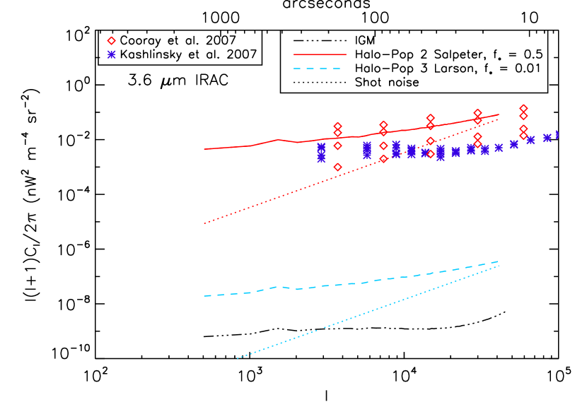
Figure 16: Our models for the angular power spectra at $3.6$ $\mu{\rm m}$ (halo+IGM) are compared with observations from Kashlinsky et al. (2007c) (their Figure 1, lower panel, shown as the blue asterisks) and from Cooray et al. (2007) (their Figure 1, images A, B, C, and D, with varying foreground galaxy cuts) shown as red diamonds. Most of our models lie beneath current observations. The mean intensity produced by Pop II stars with a Salpeter initial mass spectrum and $f_{*}=0.5$ is $\nu I_{\nu}=15.1$  nW m^-2 sr^-1, which is over current observations. For Pop III stars with a Larson initial mass spectrum and $f_{*}=0.01$, $\nu I_{\nu}=0.182$  nW m^-2 sr^-1, which is allowed by observations (for more on the mean intensity, see section 9).

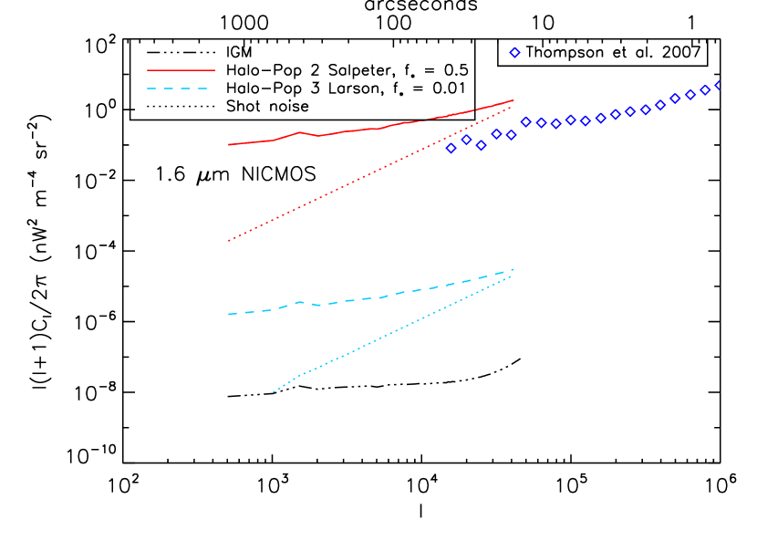
Figure 17: Our models for the angular power spectra (halo+IGM) are compared with observations from Thompson et al. (2007a) (for all sources deleted) at $1.6$ $\mu{\rm m}$, which are shown by the blue diamonds. Again, most of our models lie beneath current observations. As in the case at $3.6\mu{\rm m}$, the mean intensity from Pop II stars with a Salpeter initial mass spectrum and $f_{*}=0.5$ is high at $\nu I_{\nu}=60.1$  nW m^-2 sr^-1, while the mean intensity for Pop III stars with a Larson initial mass spectrum and $f_{*}=0.01$ is $\nu I_{\nu}=0.802$  nW m^-2 sr^-1.

Cooray et al. (2007) observed the NIRB using IRAC at 3.6 $\mu{\rm m}$. They masked the image to cut out faint, low redshift galaxies. In their most extensive masked image, they masked IRAC sources down to a magnitude of 20.2 in addition to galaxies in ACS catalog. They also discarded pixels that had a flux $4\sigma$ above the mean.

Thompson et al. (2007a) also made observations of the fluctuations of the NIRB using the Near Infrared Camera and Multi-Object Spectrometer (NICMOS) camera on the Hubble Space Telescope at 1.1 and 1.6 $\mu{\rm m}$. The effects of zodiacal light were removed by dithering the camera. After removing galaxies down to the fainter ACS and NICMOS detection limit, fluctuation power dropped two orders of magnitude in comparison to an earlier paper by Kashlinsky et al. (2002). Therefore, Thompson et al. (2007a) confirmed that the observed fluctuations reported by Kashlinsky et al. (2002) in the 2MASS data are from low redshift galaxies ($z<8$) (although they are unable to rule out contributions from galaxies in $8<z<13$). Yet, they concluded that an excess fluctuation power in the NIRB of about $1-2$ nW m^-2 sr^-1 could still be from the first stars. Their methodology would miss fluctuations that are flat on scales above $100^{\prime\prime}$ or clumped on scales of a few arc minutes.

Our models are compared to the observations at $3.6$ $\mu{\rm m}$ by Kashlinsky et al. (2007c, 2005) and Cooray et al. (2007) in Figures 16 and to observations at $1.6$ $\mu{\rm m}$ from Thompson et al. (2007a) in Figure 17. For these observations, it is safe to treat them as “upper limits,” as additional foreground contamination might still exist. At $3.6$ $\mu{\rm m}$, most of our predictions for the angular power spectra are below the current observations, and are therefore still viable candidates. At $1.6$ $\mu{\rm m}$ we see similar results. Therefore, it seems likely that early stars contribute at very low levels to the fluctuations in NIRB. Of course, other factors, such as the star formation time scale and the minimum redshift that star formation occurs at, $z_{\rm end}$, can also affect which models can agree with observations.

Missions currently underway and future, more detailed experiments can make better observations of the NIRB. AKARI (previously known as ASTRO-F) observed in 13 bands from 2-160 $\mu{\rm m}$ (Matsuhara et al., 2008). The Cosmic Infrared Background Experiment (CIBER) will be able to obtain the power spectrum from $7^{\prime\prime}$ to 2 degrees. Combined with AKARI and Spitzer, fluctuations 100 times fainter than IRTS/DIRBE will be able to be observed. CIBER has two dual wide field imagers at 0.9 and 1.6 $\mu{\rm m}$. An improved CIBER II will also measure fluctuations in four bands from 0.5 to 2.1 $\mu{\rm m}$. This experiment will be pivotal to determine if the fluctuations observed are from the first galaxies or have a more local origin (Bock et al., 2006; Cooray et al., 2009). Predictions for the sensitivity of CIBER I and II are shown in Figure 18 for both 0.9 and 1.6 $\mu{\rm m}$ (I and H-Band respectively) (Cooray et al., 2009; Bock et al., 2006). The sensitivity of CIBER will be much better than any of the current observations, but still many of our models lie beneath detection limits.

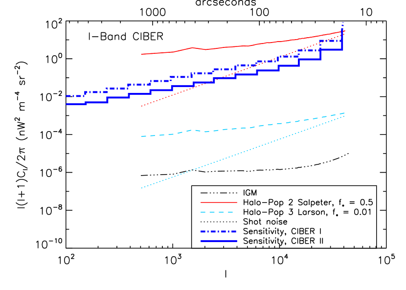
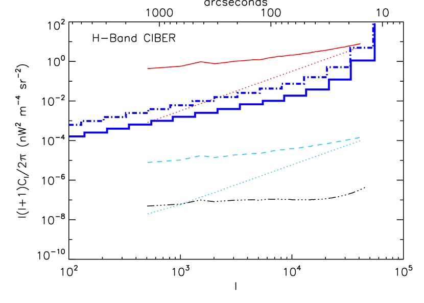
Figure 18: Our models of the angular power spectrum (halos and the IGM) compared with the sensitivities of upcoming CIBER missions (shown as the stepped blue lines) from Cooray et al. (2009). CIBER will increase sensitivity of measured fluctuations, but still many of our models will lie beneath the detection limit.

9 ADDITIONAL CONSTRAINTS FROM THE MEAN INTENSITY OF THE NEAR INFRARED BACKGROUND

In addition to fluctuations, measurements have been taken of the mean intensity of the NIRB. Because these measurements rely on an accurate subtraction of the zodiacal light, measurements of the mean intensity of the NIRB are more difficult to perform. Currently, the interpretation of these measurements is still highly controversial. Measurements of the excess in the NIRB (NIRBE) started out high ($70$ nW m^-2 sr^-1) (Matsumoto et al., 2005) and have since declined. The most recent measurements are lower. Kashlinsky et al. (2007b) report that the mean intensity of the NIRBE must be greater than 1 nW m^-2 sr^-1 to be consistent with fluctuations at 3.6 and 4.5 $\mu{\rm m}$. Thompson et al. (2007a) report a residual NIRBE of $0.0^{+3}_{-0.3}$ at 1.1 and 1.6 $\mu{\rm m}$. Fluctuations measured by Cooray et al. (2007) imply that the mean NIRB cannot be much more than 0.5 nW m^-2 sr^-1 at 3.6 $\mu{\rm m}$. Using these limits, can we put additional constrains on the first stars?

We calculate the mean intensity of NIRB from (Peacock, 1999)

$$I_{\nu}=\frac{c}{4\pi}\int\frac{dz\,p([1+z]\nu,z)}{H(z)(1+z)},$$ (41)

where $\nu$ is the observed frequency and $p(\nu,z)$ is given by Eq. (2). The star formation rate contained in $p(\nu,z)$, is given by $\dot{\rho}_{*}(z)=\rho_{*}(z)/t_{\rm SF}(z)$, where

$$\rho_{*}(z)=f_{*}\frac{\Omega_{b}}{\Omega_{m}}\bar{\rho}_{M}^{\rm halo}(z),$$ (42)

where $\bar{\rho}_{M}^{\rm halo}(z)$ is the mean mass density collapsed into halos taken from the simulation (which has the minimum halo mass of $2.2\times 10^{9}~{}M_{\sun}$), and is shown in the right panel of Figure 6. For the star formation timescale, we use $t_{\rm SF}=20~{}{\rm Myr}$, so that we can calculate the mean NIRB for models that are compatible with the WMAP data. The star formation rates with various star formation efficiencies are given in Table 3.

$f_{*}$	$\dot{\rho}_{*}(z=6)$	$\dot{\rho}_{*}(z=10)$	$\dot{\rho}_{*}(z=15)$
0.2	$1.9$	$3.7\times 10^{-2}$	$1.0\times 10^{-4}$
0.01	$9.6\times 10^{-2}$	$1.9\times 10^{-3}$	$5.1\times 10^{-6}$
0.001	$9.6\times 10^{-3}$	$1.9\times 10^{-4}$	$5.1\times 10^{-7}$

Table 3: Values of the star formation rate computed from our simulation, $\dot{\rho}_{*}$, in units of $M_{\sun}$ yr^-1 Mpc^-3. We have used the star formation timescale of $t_{\rm SF}=20~{}{\rm Myr}$.

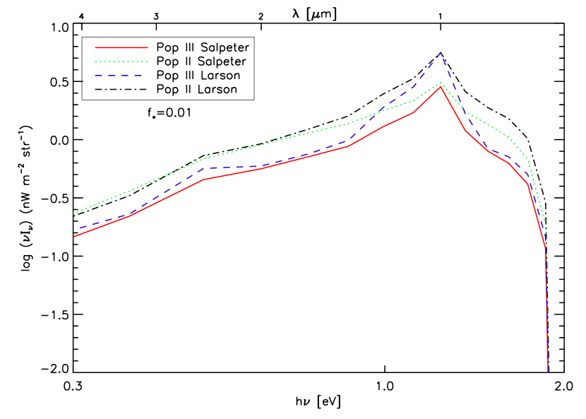
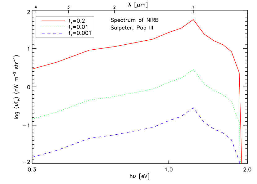
Figure 19: Spectra of the NIRBE from various populations of stars over a redshift range of 6 to 15. (Left panel) Changing initial mass spectrum and metallicity of the stars for a given star formation efficiency, $f_{*}=0.01$. (Right panel) Changing the star formation efficiency for Population III stars with a Salpeter initial mass spectrum. Models with high star formation efficiency, $f_{*}=0.2$, produce too high NIRB, and can be ruled out by the current upper limits from observations. Note that if we divided these curves by $f_{*}$, they would become identical. In other words, these curves differ solely due to the varying values of $f_{*}$.

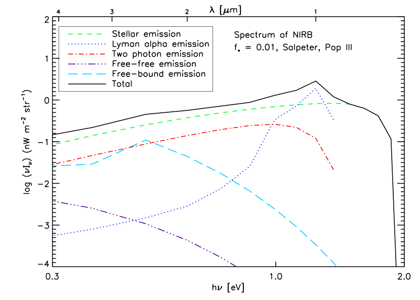
Figure 20: Spectra of the NIRBE and how each component contributes to the overall intensity, over a redshift range of 6 to 15.

We can now calculate the mean intensity of NIRB for our models with various stellar populations and values of $f_{*}$. The value of $f_{\rm esc}$ does not matter here because when calculating the mean intensity - it does not matter where the photons are coming from - the halo itself or the IGM surrounding the halo (Fernandez & Komatsu, 2006). The spectra of NIRB from various populations of stars (with varying mass, metallicity, and $f_{*}$) over the redshift range of $z=6-15$ (using simulation data up to the redshift $14.6$) are shown in Figure 19, and their numerical values (integrated over $1-2~{}\mu{\rm m}$) are tabulated in Table 4. We also show the spectra of each radiation process in Figure 20. Finally, we show the mean intensity from two redshift bins, $z=6-10$ and $10-15$, in Figure 21. Lower redshift stars clearly dominate over stars at higher redshifts. This, combined with a sharp break due to the Lyman limit as well as a bump due to the Lyman-$\alpha$ line, may be used to constrain $z_{\rm end}$.

$f_{*}$	Redshift Range	$\nu I_{\nu}$
		Pop III Larson	Pop III Salpeter	Pop II Larson	Pop II Salpeter
0.2	$6-15$	$32.2$	$22.9$	$43.2$	$32.2$
0.01		$1.61$	$1.15$	$2.16$	$1.61$
0.001		$0.161$	$0.115$	$0.216$	$0.161$

Table 4: Values of the mean background intensity, $\nu I_{\nu}$, in units of nW m^-2 sr^-1 for stars with different star formation efficiencies. The mean is calculated as an average of $\nu I_{\nu}$ over 1 to 2 $\mu{\rm m}$.

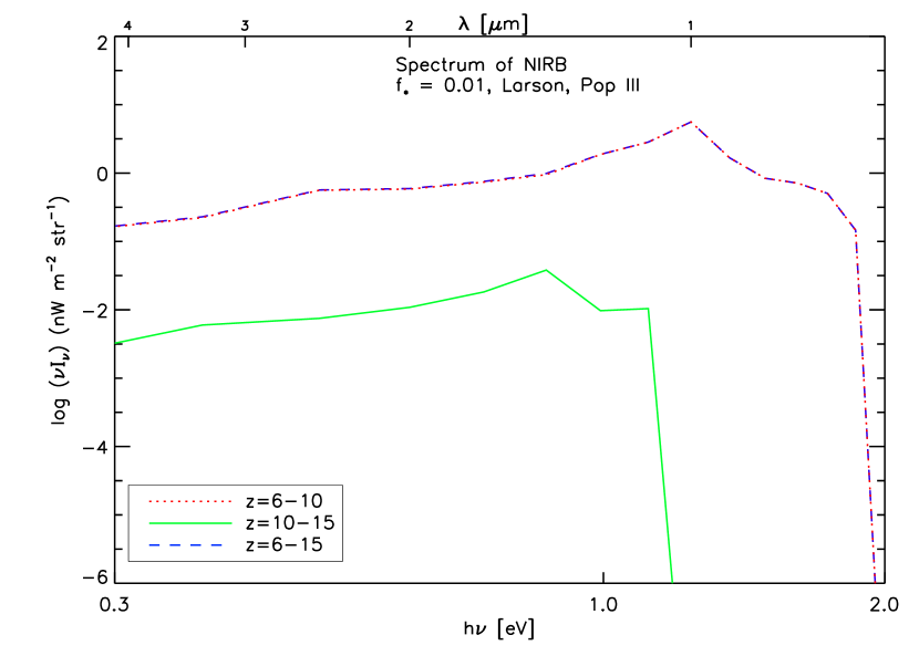
Figure 21: Spectra of the NIRBE for populations of stars over two redshift bins, $z=6-10$ and $10-15$.

Assuming that our equation for the star formation rate is accurate up to high redshifts, and using the parameters of this simulation, we can put constraints on the populations of first stars. If we take our upper limit for the mean intensity of the NIRBE to be $3$ nW m^-2 sr^-1 (the upper limit from Thompson et al. (2007a)), we can rule out most populations with high star formation efficiencies ($f_{*}=0.2$), unless star formation is constrained to only high redshifts. This is consistent with our fluctuation analysis - some of our models with high $f_{*}$ would produce angular power spectra above the levels observed. If the star formation efficiency is very low, say, $f_{*}=0.001$, then the mean background would be too small to detect. Most of the change in the amplitude of the NIRBE is from a change in the star formation efficiency $f_{*}$, while the metallicity and initial mass spectra of the stars affect the shape of the spectra. Therefore, an accurate measurement of the mean NIRBE can give information on the star formation efficiency. Further constraints on the metallicity and mass may be possible with more precise observations in the future.

10 PREDICTIONS FOR FRACTIONAL ANISOTROPY

As we have seen, the magnitude of the predicted angular power spectrum depends on various parameters such as $f_{*}$, $t_{\rm SF}$, $f_{\rm esc}$, and the initial mass spectrum. However, as the mean intensity also depends on these quantities, one may hope that the ratio of the power spectrum and the mean intensity squared would depend much less on these astrophysical parameters.

Ignoring the IGM contribution and rewriting the halo contribution given by equation (37), we get

$$C_{l} = \frac{c}{(4\pi)^{2}}\left(f_{*}\frac{\Omega_{b}}{\Omega_{m}}\right)^{2}\int\frac{dz}{H(z)r^{2}(z)(1+z)^{4}}$$ (43)

$$\times\left[\bar{\rho}_{M}^{halo}(z)\left\{\bar{l}^{*}(z)+(1-f_{\rm esc})\left[\bar{l}^{ff}(z)+\bar{l}^{fb}(z)+\bar{l}^{2\gamma}(z)+\bar{l}^{\rm Ly\alpha}(z)\right]\right\}\right]^{2}$$

$$\times b^{2}_{eff}\left(k=\frac{l}{r(z)},z\right)P_{\rm lin}\left(k=\frac{l}{r(z)},z\right).$$

By rewriting and averaging equation (41) over a band, we get

$$I = \frac{c}{4\pi}\left(f_{*}\frac{\Omega_{b}}{\Omega_{m}}\right)\int\frac{dz}{H(z)(1+z)}$$ (45)

$$\times\bar{\rho}_{M}^{halo}(z)\left[\bar{l}^{*}(z)+\bar{l}^{ff}(z)+\bar{l}^{fb}(z)+\bar{l}^{2\gamma}(z)+\bar{l}^{\rm Ly\alpha}(z)\right].$$

Therefore, in the ratio $C_{l}/I^{2}$, $f_{*}$ and $t_{\rm SF}$ (which is related to $\bar{l}^{\alpha}$ as $\bar{l}^{\alpha}\propto 1/t_{\rm SF}$) cancel out exactly. The dependence on the initial mass spectrum, $f(m)$, which determines $\bar{l}^{\alpha}$ via integral, nearly cancels out. However, the dependence on $f_{\rm esc}$ does not cancel out: the power spectrum depends on $f_{\rm esc}$, whereas the mean intensity does not. Therefore, we conclude that the ratio depends primarily on $f_{\rm esc}$. In Figure 22 we show the fractional anisotropy, $\delta I/I\equiv\sqrt{l(l+1)C_{l}/(2\pi I^{2})}$, for various infrared bands. Here, $I$ is the mean intensity averaged over the bands defined in Table 5, which are taken from Sterken & Manfroid (1992). We assume a rectangular bandpass. The upper curves are for $f_{\rm esc}=0.19$, while the lower curves are for $f_{\rm esc}=1$, which is consistent with the expectation: the ratio of the angular power spectrum to the mean intensity is lower for a higher $f_{\rm esc}$. We have checked that the ratio is nearly the same for different mass spectra for $f_{\rm esc}=0$, in which case the dependence on $\bar{l}(z)$ nearly cancels out.

Note that for $f_{\rm esc}=0$ the ratio, $C_{l}/I^{2}$, may be regarded as an weighted average of $b^{2}_{eff}(l/r)P_{\rm lin}(l/r)$. We find $\delta I/I=\sqrt{l(l+1)C_{l}/(2\pi I^{2})}\approx 10^{-2}$ with a weak dependence on $l$, i.e., $\delta I/I\propto l^{0.25}$. In other words, the expected fractional anisotropy of the near infrared background is of order a few percent for $f_{\rm esc}=0$, and can be lower by a factor of a few for $f_{\rm esc}=1$.

Band	Center (microns)	Waveband (microns)
J	1.25	1.1-1.4
H	1.65	1.5-1.8
K	2.2	2.0-2.4
L	3.5	3.0-4.0
M	4.8	4.6-5.0

Table 5: Band definitions used for infrared bands. These are given in Table 16.2 in Sterken & Manfroid (1992).

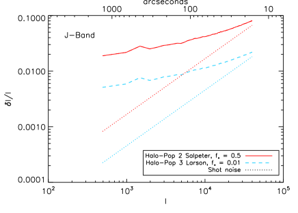
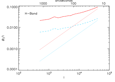
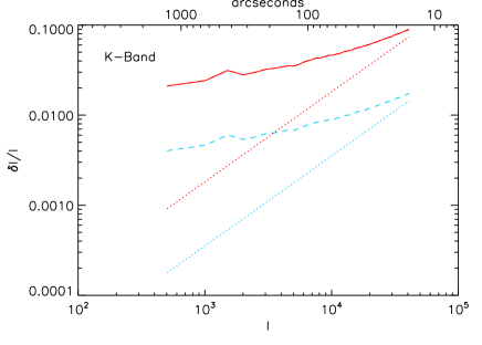
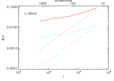
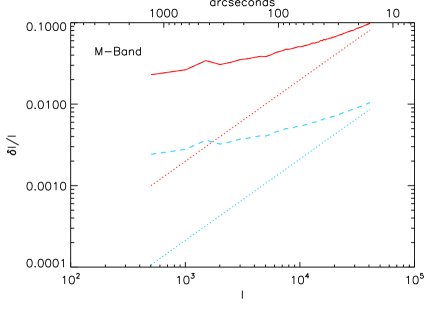
Figure 22: Fractional anisotropy, $\delta I/I=\sqrt{l(l+1)C_{l}/(2\pi I^{2})}$, for different infrared bands, as labeled, versus the wavenumber $l$. This quantity depends primarily on the escape fraction, $f_{\rm esc}$. The upper curves are for $f_{\rm esc}=0.19$, while the lower curves are for $f_{\rm esc}=1$. Therefore, the expected fractional anisotropy of the near infrared background is of order of a few percent for $f_{\rm esc}=0$, and can be lower by a factor of a few for $f_{\rm esc}=1$. Note that the dependence on $f_{*}$ and $t_{\rm SF}$ cancels out exactly in $\delta I/I$.

11 DISCUSSION AND CONCLUSIONS

Any detection or non-detection of fluctuations in NIRB can give us information on stars forming at high redshifts, stars that could have helped to reionize the universe. The escape fraction of ionizing photons, the star formation efficiency, and the mass and metallicity of the stars can affect the amplitude and shape of the angular power spectrum of fluctuations in NIRB.

We modeled the angular power spectrum from halos and the surrounding IGM by combining the analytic formulas for the luminosity of halos and the IGM with $N$-body simulations coupled with radiative transfer for several different populations of stars. Shot noise is a major contributor to the angular power spectrum of halos at small scales, so it is important to include larger scales in observations to minimize the component of shot noise.

The star formation efficiency has a significant effect on the amplitude of the angular power spectrum, with the amplitude of the angular power spectrum being proportional to $f_{*}^{2}$. For a fixed $f_{\gamma}/t_{\rm SF}=f_{\rm esc}f_{*}N_{i}/t_{\rm SF}$ (i.e., for a given reionization history), a combination of parameters that maximize the star formation efficiency, $f_{*}$, give the largest NIRB power spectrum; thus, the stars that are less massive and have more metals (smaller $N_{i}$), and are in halos with a lower escape fraction (smaller $f_{\rm esc}$) will all increase the amplitude of the NIRB angular power spectrum. In general, the amplitude of the angular power spectrum of the halos (and the mean NIRBE) is mostly dominated by $f_{*}$, while the angular power spectrum of the IGM can probe the ionization history though the factor $f_{\gamma}/t_{SF}$.

If we do not fix the reionization history, there are other parameters that can change the amplitude of the angular power spectrum significantly. The angular power spectrum is inversely proportional to the star formation time scale squared, $C_{l}\propto 1/t_{\rm SF}^{2}$. This uncertainty in the star formation time scale can be directly related to our uncertainty in the mass to light ratio of galaxies, for $t_{\rm SF}\propto M_{h}/L_{h}$. As changes in $t_{\rm SF}$ result in different reionization histories (for a given $f_{\gamma}$), the other tracers of reionization, e.g., the electron-scattering optical depth measured by the WMAP satellite and the abundance of Lyman-$\alpha$ emitting galaxies, should help narrow down a range of magnitudes of the NIRB fluctuations that are consistent with what we already know about the cosmic reionization.

The angular power spectrum of the IGM is typically a minor contributor to the overall fluctuations; however, the IGM contribution can be comparable to the halo contribution (the stellar contribution as well as the nebular contribution from within the halo), especially if the escape fraction of ionizing photons from halos is high. In the limit that $f_{\rm esc}$ is close to unity, we expect $C_{l}^{\rm IGM}/C_{l}^{\rm halo}\propto f_{\rm esc}^{2}$, as $C_{l}^{\rm halo}$ would be completely dominated by the stellar emission. One can even make the IGM contribution dominate over the halo contribution by increasing $t_{\rm SF}$, which suppresses the halo contribution as $C_{l}^{\rm halo}\propto t_{\rm SF}^{-2}$, and leads to a delay in the reionization. Yet, this would not change the IGM power spectrum significantly, as the IGM luminosity power spectrum saturates when the ionization fraction reaches $X_{e}\sim 0.5$. Of course, we need to make sure that such a model can still complete the reionization by $z\sim 6$, and can reproduce the electron-scattering optical depth measured by WMAP.

The redshift at which the formation of stars contributing to NIRB ends, $z_{\rm end}$, can also change the amplitude of the angular power spectrum significantly. Changing $z_{\rm end}$ affects not only the amplitude of the angular power spectrum, but also the shape. The attenuation of Lyman-$\alpha$ photons for the most part, does not affect the angular power spectrum of the halos greatly, but could affect the amplitude of the IGM by about a factor of 2.

Previous estimates of the angular power spectrum of the NIRB by Cooray et al. (2004) neglected to account for nonlinear bias. For our simulation with the minimum halo mass of $2.2\times 10^{9}~{}M_{\sun}$, the nonlinear bias is large enough to change the prediction for the shape of the angular power spectrum qualitatively: a turnover of $l(l+1)C_{l}$ at $l\sim 10^{3}$ that was predicted by Cooray et al. (2004) is not seen in our calculation, and the shape of the clustering component (i.e., minus the shot noise), is consistent with a pure power law, $l(l+1)C_{l}\propto l^{0.5}$.

Note that our results for the shape of the angular power spectrum are valid for the minimum halo mass of $M_{\rm min}=2.2\times 10^{9}\>M_{\sun}$. The non-linear bias would be smaller for smaller mass halos. For example, the simulation carried out by Trac & Cen (2007) resolves halos down to a smaller mass, $M_{\rm min}=6\times 10^{7}~{}h^{-1}~{}M_{\sun}$, and would therefore find a smaller average bias. The halo bias is mass dependent, more massive halos being more strongly biased. The effective linear bias, $b_{\rm eff,lin}$, is the integral of the linear halo bias for a given mass, $b_{1}(M_{h})$, times the mass function weighted by mass above a certain minimum mass, i.e., $b_{\rm eff,lin}=[\int_{M_{\rm min}}^{\infty}dM_{h}~{}M_{h}(dn_{h}/dM_{h})b_{1}(M_{h})]/[\int_{M_{\rm min}}^{\infty}dM_{h}~{}M_{h}(dn_{h}/dM_{h})]$. As there are many more halos at lower masses, lowering $M_{\rm min}$ would result in a lower average bias. As the degree of the non-linear bias increases as the linear bias increases, one would find a smaller non-linear bias for a lower $M_{\rm min}$. Therefore, we might still see a turnover if these smaller halos are bright enough to contribute to the NIRB.

However, the real situation would be more complex than the above picture. In Iliev et al. (2007), we also performed reionization simulations which resolve source halos down to this lower minimum mass of $\sim 10^{8}~{}M_{\sun}$. There, however, unlike Trac & Cen (2007), we took account of the fact that those small-mass ($\lesssim 10^{9}~{}M_{\sun}$) halos are subject to Jeans filtering, and thus their star formation is suppressed if they reside within the ionized regions. The suppression occurs disproportionately on the low-mass halos clustered around the high-density peaks (which are the first to be ionized). Therefore, the ultimate effect may not be as large as one might think by just including all halos down to $\sim 10^{8}~{}M_{\sun}$. While it is plausible that there may be a turn-over, it is also quite plausible that the location of the turn-over would be on a smaller scale than what would be predicted by the linear bias model.

This can, in principle, be studied using higher-resolution simulations like those in Iliev et al. (2007) that include the Jeans filtering effect, but the simulation box size of $35~{}h^{-1}~{}{\rm Mpc}$ there is not quite large enough to give a reliable statistical measure of the large-scale structure and angular fluctuations in which we are interested. Towards that end, we have more recently performed a new set of large-box, higher-resolution simulations that include the Jeans filtering effect, reported in Shapiro et al. (2008) and Iliev et al. (2008a). We shall present results on the NIRB from these higher-resolution simulations elsewhere. In any case, the above consideration suggests that the shape of the angular power spectrum gives us important information about the nature of sources contributing to NIRB as well as the physics of cosmic reionization.

Current observations seem to favor low levels of both the fluctuations and the mean NIRB due to the high-$z$ (i.e., $z\gtrsim 7$) sources. The current observations of the mean intensity of the NIRB seem to rule out high levels of $f_{*}$, i.e., $f_{*}\gtrsim 0.2$. Most of our models for fluctuations still lie beneath the current observations of the fluctuations of the NIRB. The upcoming CIBER missions will improve the sensitivity of observations, but many of our models still lie below their sensitivity limits. Nevertheless, these new observations should be able to put tighter constraints on which high-$z$ galaxy populations are allowed and which are ruled out. Given the lack of direct observational probes of high-$z$ galaxy populations contributing to the cosmic reionization, the NIRB continues to offer invaluable information regarding the physics of cosmic reionization that is difficult to probe by other means.

We would like to thank Asantha Cooray, Daniel Eisenstein, Donghui Jeong, Yi Mao, and Rodger Thompson for helpful discussions. This study was supported by Spitzer Space Telescope theory grant 1310392, NSF grant AST 0708176, NASA grants NNX07AH09G and NNG04G177G, Chandra grant SAO TM8-9009X, and Swiss National Science Foundation grant 200021-116696/1. ERF acknowledges support from the University of Colorado Astrophysical Theory Program through grants from NASA (NNX07AG77G) and NSF (AST07-07474). EK acknowledges support from an Alfred P. Sloan Research Fellowship.

Appendix A Derivation of Angular Power Spectrum of NIRB Fluctuations

The observed intensity (energy received per unit time, unit area, unit solid angle, and unit frequency) of the NIRB toward a direction on the sky $\hat{\mathbf{n}}$, $I_{\nu}(\hat{\mathbf{n}})$, is related to the spatial distribution of the volume emissivity (luminosity emitted per frequency per comoving volume) at various redshifts, $p(\nu,{\mathbf{x}},z)$, as (Peacock, 1999, p.91)

$$I_{\nu}(\hat{\mathbf{n}})=\frac{c}{4\pi}\int dz\frac{p[\nu(1+z),\hat{\mathbf{n}}r(z),z]}{H(z)(1+z)},$$ (A1)

where $r(z)=c\int_{0}^{z}dz^{\prime}/H(z^{\prime})$ is the comoving distance. The band-averaged intensity is then given by

$$I(\hat{\mathbf{n}}) \equiv \int_{\nu_{1}}^{\nu_{2}}d\nu~{}I_{\nu}(\hat{\mathbf{n}})=\frac{c}{4\pi}\int dz\frac{\int_{\nu_{1}}^{\nu_{2}}d\nu~{}p[\nu(1+z),\hat{\mathbf{n}}r(z),z]}{H(z)(1+z)}$$ (A2)

$$= \frac{c}{4\pi}\int dz\frac{\int_{\nu_{1}(1+z)}^{\nu_{2}(1+z)}d\tilde{\nu}~{}p[\tilde{\nu},\hat{\mathbf{n}}r(z),z]}{H(z)(1+z)^{2}},$$ (A3)

where $\tilde{\nu}=\nu(1+z)$. Note that the denominator now contains $(1+z)^{2}$ instead of $(1+z)$.

Now, using the luminosity density integrated over bands, $\rho_{L}({\mathbf{x}},z)\equiv\int_{\nu_{1}(1+z)}^{\nu_{2}(1+z)}d\nu~{}p(\nu,{\mathbf{x}},z)$, we obtain

$$I(\hat{\mathbf{n}})=\frac{c}{4\pi}\int dz\frac{\rho_{L}[\hat{\mathbf{n}}r(z),z]}{H(z)(1+z)^{2}}.$$ (A4)

The spherical harmonic transform of $I(\hat{\mathbf{n}})$, $a_{lm}=\int d\hat{\mathbf{n}}~{}I(\hat{\mathbf{n}})Y_{lm}^{*}(\hat{\mathbf{n}})$, is then related to the three-dimensional Fourier transform of $\rho_{L}({\mathbf{x}},z)$, $\tilde{\rho}_{L}({\mathbf{k}},z)=\int d^{3}{\mathbf{x}}~{}\rho_{L}({\mathbf{x}},z)e^{i{\mathbf{k}}\cdot{\mathbf{x}}}$ (the inverse transform is $\rho({\mathbf{x}},z)=\int d^{3}{\mathbf{k}}/(2\pi)^{3}~{}\tilde{\rho}_{L}({\mathbf{k}},z)e^{-i{\mathbf{k}}\cdot{\mathbf{x}}}$), as,

$$a_{lm}=\frac{c}{4\pi}\int\frac{dz}{H(z)(1+z)^{2}}\left[4\pi(-i)^{l}\int\frac{d^{3}{\mathbf{k}}}{(2\pi)^{3}}\tilde{\rho}_{L}({\mathbf{k}},z)j_{l}[kr(z)]Y_{lm}^{*}(\hat{\mathbf{k}})\right],$$ (A5)

where we have used Rayleigh’s formula:

$$e^{-i{\mathbf{k}}\cdot{\hat{\mathbf{n}}}r(z)}=4\pi\sum_{lm}(-i)^{l}j_{l}[kr(z)]Y_{lm}^{*}(\hat{\mathbf{k}})Y_{lm}(\hat{\mathbf{n}}).$$ (A6)

The angular power spectrum, $C_{l}=\langle|a_{lm}|^{2}\rangle$, is then given by ($\langle\rangle$ is the statistical ensemble average)

$$C_{l}=\left(\frac{c}{4\pi}\right)^{2}\int\frac{dz}{H(z)(1+z)^{2}}\int\frac{dz^{\prime}}{H(z^{\prime})(1+z^{\prime})^{2}}\left[\frac{2}{\pi}\int k^{2}dk~{}P_{L}(k,z)j_{l}[kr(z)]j_{l}[kr(z^{\prime})]\right],$$ (A7)

where we have used the definition of the luminosity-density power spectrum (Eq. (24)), and the normalization of the spherical harmonics, $\int d\hat{\mathbf{k}}Y_{lm}(\hat{\mathbf{k}})Y^{*}_{lm}(\hat{\mathbf{k}})=1$.

Now, when $l\gg 1$, the integral within the square bracket can be approximated as

$$\frac{2}{\pi}\int k^{2}dk~{}P_{L}(k,z)j_{l}[kr(z)]j_{l}[kr(z^{\prime})]\approx\frac{\delta\left[r(z)-r(z^{\prime})\right]}{r^{2}(z)}P_{L}\left(k=\frac{l}{r(z)},z\right).$$ (A8)

Therefore,

$$C_{l} \approx \left(\frac{c}{4\pi}\right)^{2}\int\frac{dz}{H(z)(1+z)^{2}}\int dr^{\prime}\frac{dz^{\prime}/dr^{\prime}}{H(z^{\prime})(1+z^{\prime})^{2}}\frac{\delta(r-r^{\prime})}{r^{2}(z)}P_{L}\left(k=\frac{l}{r(z)},z\right)$$ (A9)

$$= \frac{c}{(4\pi)^{2}}\int\frac{dz}{H(z)r^{2}(z)(1+z)^{4}}P_{L}\left(k=\frac{l}{r(z)},z\right),$$

where $r=r(z)$ and $r^{\prime}=r(z^{\prime})$, and we have used $dz/dr=H(z)/c$. This is Eq. (37).

On the other hand, if one chooses to calculate $C_{l}$ from a pair of $I_{\nu}(\hat{\mathbf{n}})$ and $I_{\nu^{\prime}}(\hat{\mathbf{n}})$ instead of a pair of the band-averaged intensities $I(\hat{\mathbf{n}})$, then $(1+z)^{4}$ in the denominator of Eq. (A9) becomes $(1+z)^{2}$:

$$C_{l}^{\nu\nu^{\prime}}=\frac{c}{(4\pi)^{2}}\int\frac{dz}{H(z)r^{2}(z)(1+z)^{2}}P_{p}\left(\nu(1+z),\nu^{\prime}(1+z);k=\frac{l}{r(z)},z\right),$$ (A10)

where $P_{p}(\nu,\nu^{\prime};k,z)$ is the power spectrum of the volume emissivity, $p(\nu,z)$. Eq. (A10) agrees with Eq. (10) of Cooray et al. (2004). Note that their $j_{\nu}$ is $p(\nu)/(4\pi)$ in our notation, which explains the absence of $1/(4\pi)^{2}$ in their Eq. (10). However, this result does not agree with Eq. (3) of Kashlinsky et al. (2004), which originates from Eq. (11) of Kashlinsky & Odenwald (2000). (See also Eq. (14) of Kashlinsky (2005).) Kashlinsky et al.’s formula has $(1+z)$ in the denominator of Eq. (A10) instead of $(1+z)^{2}$, and thus it misses one factor of $1/(1+z)$. We were unable to trace the cause of this discrepancy. It is therefore possible that Kashlinsky et al. (2004) over-estimated $C_{l}$ by a factor of $\sim 10$. As they have not taken into account a short lifetime of massive stars in their calculations (i.e., they used Eq. (7) instead of Eq. (6)), which yields another factor of $\sim 100$ in $C_{l}$, it is possible that they over-estimated $C_{l}$ by a factor of $\sim 10^{3}$.

References

- Ahn & Shapiro (2007) Ahn, K., & Shapiro, P. R. 2007, MNRAS, 375, 881
- Ahn et al. (2009) Ahn, K., Shapiro, P. R., Iliev, I. T., Mellema, G., & Pen, U.-L. 2009, ApJ, 695, 1430
- Bock et al. (2006) Bock, J., et al. 2006, New Astron, 50, 215
- Cambresy et al. (2001) Cambresy, L., Reach, W. T., Beichman, C. A., & Jarrett, T. H. 2001, ApJ, 555, 563
- Chary, Cooray & Sullivan (2008) Chary, R., Cooray, A., & Sullivan, I. 2008, ApJ, 681, 53
- Cooray & Sheth (2002) Cooray, A., & Sheth, R. 2002, Phys. Rep, 372, 1
- Cooray & Yoshida (2004) Cooray, A., & Yoshida, N. 2004, MNRAS, 351, L71
- Cooray et al. (2004) Cooray, A., et al. 2004, ApJ, 606, 611
- Cooray et al. (2007) Cooray, A., et al. 2007, ApJ, 659, L91
- Cooray et al. (2009) Cooray, A., et al. 2009, arXiv:0904.2016
- Dunkley et al. (2009) Dunkley, J., et al. 2009, ApJS, 180, 306
- Dwek & Arendt (1998) Dwek, E., & Arendt, R. G. 1998, ApJ, 508, L9
- Fernandez & Komatsu (2006) Fernandez, E. R., & Komatsu, E. 2006, ApJ, 646, 703
- Fernandez & Komatsu (2008) Fernandez, E. R., & Komatsu, E. 2008, MNRAS, 384, 1363
- Ferrara (1998) Ferrara, A. 1998, ApJ, 499, 17
- Gorjian, Wright & Chary (2000) Gorjian, V., Wright, E. L., & Chary, R. R. 2000, ApJ, 536, 550
- Haiman, Abel & Rees (2000) Haiman, Z., Abel T., & Rees M. J. 2000, ApJ, 534, 11
- Haiman, Rees & Loeb (1997) Haiman, Z., Rees M. J., & Loeb A. 1997, ApJ, 476, 458
- Iliev et al. (2008a) Iliev, I. T., Mellema, G., Merz, H., Shapiro, P. R., & Pen, U.-L. 2008a, in TeraGrid08, in press (arXiv:0806.2887)
- Iliev et al. (2006) Iliev, I. T., Mellema, G., Pen, U.-L., Merz, H., Shapiro, P. R., & Alvarez, M. A. 2006, MNRAS, 369, 1625
- Iliev et al. (2008b) Iliev, I. T., Mellema, G., Pen, U.-L., Bond, J. R., & Shapiro, P. R., 2008b, MNRAS, 384, 863
- Iliev et al. (2007) Iliev, I. T., Mellema, G., Shapiro, P. R., & Pen, U.-L. 2007, MNRAS, 376,534
- Jeong & Komatsu (2009) Jeong, D., & Komatsu, E. 2009, ApJ, 691, 569
- Jing (2005) Jing, Y. P. 2005, ApJ, 620, 559
- Johnson, Grief & Bromm (2008) Johnson, J., Grief, T., & Bromm, V. 2008, arXiv:0802.0207
- Kashlinsky (2005) Kashlinsky, A. 2005, PhR, 409, 361
- Kashlinsky (2006) Kashlinsky, A. 2006, astro-ph/0610943
- Kashlinsky (2007a) Kashlinsky, A. 2007a, arXiv:0709.0487
- Kashlinsky (2007b) Kashlinsky, A. 2007b, astro-ph/0701147
- Kashlinsky et al. (2004) Kashlinsky, A., Arendt, R., Gardner, J. P., Mather, J. C., & Moseley, S. H. 2004, ApJ, 608, 1
- Kashlinsky et al. (2005) Kashlinsky, A., Arendt, R. G., Mather, J., & Moseley, S. H. 2005, Nature, 438, 45
- Kashlinsky et al. (2007a) Kashlinsky, A., Arendt, R. G., Mather, J., & Moseley, S. H. 2007a, ApJ, 666, L1
- Kashlinsky et al. (2007b) Kashlinsky, A., Arendt, R. G., Mather, J., & Moseley, S. H. 2007b, ApJ, 654, L1
- Kashlinsky et al. (2007c) Kashlinsky, A., Arendt, R. G., Mather, J., & Moseley, S. H. 2007c, ApJ, 654, L5
- Kashlinsky & Odenwald (2000) Kashlinsky, A., & Odenwald, S. 2000, ApJ, 528, 74
- Kashlinsky et al. (2002) Kashlinsky, A., Odenwald, S., Mather, J., Skrutskie, M. F., & Cutri, R. M. 2002, ApJ, 579, L53
- Kogut et al. (2003) Kogut, A., et al. 2003, ApJS, 148, 161
- Komatsu et al. (2009) Komatsu, E., et al. 2009, ApJS, 180, 330
- Larson (1998) Larson, R. B. 1999, MNRAS, 301, 569
- Lejeune & Schaerer (2001) Lejeune T., Schaerer D., 2001, A&A, 336, 538L
- Loeb & Rybicki (1999) Loeb, A., & Rybicki, G. B. 1999, ApJ, 524, 527
- Machacek, Bryan & Abel (2003) Machacek, M. E., Bryan, G. L., & Abel, T. 2003, ApJ, 548, 509
- Madau, Meiksin & Rees (1997) Madau, P., Meiksin, A., & Rees, M. J. 1997, ApJ, 475, 429
- Madau & Silk (2005) Madau, P., & Silk, J. 2005, MNRAS, 359, L22
- Magliocchetti, Salvaterra, & Ferrara (2003) Magliocchetti, M., Salvaterra, R., & Ferrara, A. 2003, MNRAS, 342, L25
- Marigo et al. (2001) Marigo P., Girardi L., Chiosi C., Wood P. R., 2001, A&A, 371,152
- Matsuhara et al. (2008) Matsuhara, H., Wada, T., Matsuura, S., Nakagawa, T., Pearson, C. P., Kawada, M., & Shibai, H. 2008, ASP Conference Series, Vol 381, 507
- Matsumoto et al. (2005) Matsumoto, T., Matsuura, S., Murakami, H., Tanaka, M., Freund, M., Lim, M., Cohen, M., Kawada, M., & Noda, M. 2005, ApJ, 626, 31
- Mellema et al. (2006) Mellema, G., Iliev, I. T., Alvarez, M. A., & Shapiro, P. R. 2006, New Astron., 11, 374
- Merz, Pen & Trac (2005) Merz, H., Pen, U.-L., & Trac, H. 2005, New Astron., 10, 393
- Odenwald et al. (2003) Odenwald, S., Kashlinsky, A., Mather, J. C., Skrutskie, M. F., & Cutri, R. M. 2003, ApJ, 583, 535
- O’Shea & Norman (2008) O’Shea, B. W., & Norman, M. L. 2008, ApJ, 673, 14
- Page et al. (2007) Page, L., et al. 2007, ApJS, 170, 335
- Peacock (1999) Peacock, J. A. 1999, Cosmological Physics (Cambridge University Press), pp 91-94
- Press & Schechter (1974) Press, W. H., & Schechter, P. 1974, ApJ, 187, 425
- Ricotti et al. (2001) Ricotti, M., Gnedin, N. Y., Shull, M. J., 2001, ApJ, 560, 580
- Schaerer (2002) Schaerer D., 2002, A&A, 382, 28
- Salpeter (1955) Salpeter, E. E. 1955, ApJ, 121, 161
- Salvaterra & Ferrara (2003) Salvaterra, R., & Ferrara, A. 2003, MNRAS, 339, 973
- Santos, Bromm & Kamionkowski (2002) Santos, M. R., Bromm, V., & Kamionkowski, M. 2002, MNRAS, 336, 1082
- Spergel et al. (2003) Spergel, D. N., et al. 2003, ApJS, 148, 175
- Spergel et al. (2007) Spergel, D. N., et al. 2007, ApJS, 170, 377
- Shapiro et al. (2008) Shapiro, P. R., Iliev, I. T., Mellema, G., Pen, U.-L., & Merz, H. 2008, in The Evolution of Galaxies through the Neutral Hydrogen Window, (AIP Conf. Proc. Vol. 1035), eds. Robert Minchin & Emmanuel Momjian, 1035, 68-74 (arXiv:0806.3091)
- Spitzer (1978) Spitzer, L. 1978, Physical Processes in the Interstellar Medium (John Wiley & Sons)
- Sterken & Manfroid (1992) Sterken, Chr., & Manfroid, J. 1992, Astronomical Photometry – A Guide (Kluwer Academic Publishers: Dordrecht)
- Sullivan et al. (2007) Sullivan, I., et al. 2007, ApJ, 657, 37
- Thompson et al. (2007a) Thompson, R. I., Eisenstein, D., Fan, X., Rieke, M., & Kennicutt, R. C. 2007a, ApJ, 657, 669
- Thompson et al. (2007b) Thompson, R. I., Eisenstein, D., Fan, X., Rieke, M., & Kennicutt, R. C. 2007b, ApJ, 666, 658
- Totani et al. (2001) Totani, T., Yoshii, Y., Iwamuro, F., Maihara, T., & Motohara, K. 2001, ApJ, 550, L137
- Trac & Cen (2007) Trac, H., & Cen, R. 2007, ApJ, 671, 1
- Wise et al. (2007) Wise, J., & Abel, T. 2007, ApJ, 671, 1559
- Wright (2001) Wright, E. L. 2001, ApJ, 553, 538
- Wright & Reese (2000) Wright, E. L., & Reese, E. D. 2000, ApJ, 545, 43
- Yoshida et al. (2003) Yoshida, N., Abel, T., Hernquist, L., & Sugiyama, N. 2003, ApJ, 592, 645